Radial Basis Function Networks GPU Based Implementation

1

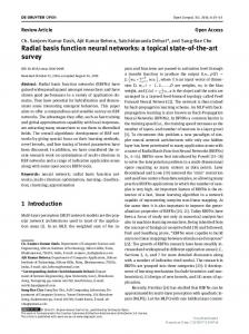
Radial Basis Function Networks GPU Based Implementation A. Brandstetter and A. Artusi

Abstract—The Neural Networks have been used in several areas, showing their potential but also their limitations. One of the main limitations is the long time required for the training process; this is not useful in the case of a fast training process being required to respond to changes in the application domain. A possible way to accelerate the learning process of a Neural Network is to implement it in hardware, but due to the high cost and the reduced flexibility of the original CPU implementation, this solution is often not chosen. Recently the power of the graphic processing unit (GPU), on the market, has increased and it has started to be used in many applications. In particular a kind of Neural Network named Radial Basis Function Network has been used extensively, proving its power. However their limiting time performances reduce their application in many areas. In this paper, we describe a GPU implementation of the entire learning process of a Radial Basis Function Network showing the ability to reduce the computational cost by about two orders of magnitude with respect to its CPU implementation. Index Terms—Graphic processing unit (GPU), Neural Networks (NN’s), Radial Basis Function Networks (RBFN’s).

I. I NTRODUCTION Neural Networks (NN’s) are used to solve complex problems in many areas like Image Processing, Computer Graphics, Pattern Recognition, Economics etc., showing their ability to improve the quality performance versus the traditional methods. Besides their good quality performance, the NN’s are limited to applications where the computation time dedicated to the learning process is not a critical issue. On the other hand, time performance is critical in many application areas. In particular in many applications where NN’s are used, it is necessary to reduce the computation time dedicated to the training process. This speed-up can be achieved with a fully parallel specially designed hardware implementation, and requires extra design overheads and this is expensive as reported in [1]. Recently graphics hardware has become competitive in terms of speed and programmability and has been started to be used for the implementation of various algorithms that are not related to Computer Graphics, and this area is named General Purpose GPU Programming (GPGPU)[2]. At this time, different architectures of NN’s are available; in this paper we will concentrate on the implementation of the entire training process used to teach a kind of multilayer perceptron named Radial Basis Function Network (RBFN). Manuscript received March 31, 2007 and revised on January 7, 2008 A. Brandstetter is with the Institute of Computer Graphics and Algorithms, Vienna University of Technology TU Wien. A. Artusi is with the Warwick Digital Laboratory at the University of Warwick UK.

We will show how it is possible to accelerate the training process by about two orders of magnitude when compared with the same learning algorithm implemented on the CPU. The paper is organised as follows: Section II describes the related work. An introducion on the RBFN and the basic learning approaches are given in Section III, a description of the GPU implementation of the RBFN is given in Section IV. Experimental results that report the time and the quality performances are in Section V, and finally conclusions and future work are discussed in Section VI II. R ELATED W ORK The interest in GPU programming has increased recently thanks to the increasing power and programmability of commonly available graphic cards. It has been shown that a variety of numerical tasks can be computed on standard graphics hardware. Kruger and Westermann used GPU shader programs to solve the Navier-Stokes equation [3]. Moravanszky gave an algorithm for matrix multiplication on the GPU [4]. Various other non-graphical applications for graphics hardware have been discussed, among them finite element analysis and fluidflow simulation. In the last two years some works have appeared that tries to explore the use of the GPU in the NN areas. Su-Oh et al. [1] proposed a GPU implementation of the multiplication between the weights and the input vectors in each layer, so called inner-product, in a multilayer perceptron. The training phase was done off-line using a CPU implementation of the training algorithm. In this way, they were able to accelerate the working phase of a multilayer perceptron in image processing and pattern recognition applications. In the same year Rolfes [5] presented a simulation on a GPU of a multilayer perceptron. Also in this case, his simulation is limited to the inner-product. In both papers the matrix multiplication is based on the methods presented in [4] [3]. Davis [6], in his Masters Thesis, revisited the inner-product implementation, for the multilayer perceptron, of Rolfes [5]. Also, he implemented the Hopfield architecture and the Adaptive Resonance Theory both based on the matrix multiplication used by [1] and [5]. Zhongwen et al. [7], presented a simulation on the GPU of Self-Organizing Maps also called Kohonen Future Maps (KFM) showing the abilty to slightly accelerate the training process of the (KFM) with respect to the original CPU implementation. Finally Chelapilla et al. [8], presented how to accelerate a Convolution Neural Network for document processing. We are not aware of any GPU simulator of the entire learning process, and not only for the inner-product, for a multilayer perceptron as the Radial Basis Function Network.

2

III. R ADIAL BASIS F UNCTION N ETWORK RBFN A. Neural Networks The base of a Neural Network (NN) is a formal neuron. It is defined as a series of inputs, a series of outputs and by a function that maps specific inputs to series of outputs [9]. NN’s consist of collections of connected formal neurons. Each formal neuron computes a simple nonlinear function f on the weighted sum of its input. The function f is referred to as activation function and its output is defined as the activation of the formal neuron. Long term knowledge is stored in the network in the form of interconnection weights that link such formal neurons. In a NN, the learning phase is a process where a set of weights are defined that produces a desired response as a reaction to certain input patterns. There are two main techniques for the learning phase: supervised learning and non–supervised learning[9]. In supervised learning the function is learned from samples which a “teacher” supplies. This set of samples, referred to as the training set, contains elements which consist of paired values of the independent (input) variable and the dependent (output) variable [10]. In the case of non– supervised learning, it reaches an internal model that captures the regularity in the inputs without taking other information into account. In this paper we refer to the supervised learning model. B. Basis functions

In the case of a non–linear model there are two more modifications if the basis function can move, change size, or if there is more than one hidden layer: •

•

There is no constraint that the centers of basis functions have to be input points; instead, determining these centers is part of the training process. Instead of a unique parameter r, every basis function has a parameter rj , the value of which is obtained during the training process.

There are two stages for the training phase: determining the basis function parameters (non-linear models), and the finding of appropriate weights.

D. Linear network models In the case of a linear model, the parameters of the basis functions are fixed, and the goal is to minimise the sum of the squared errors in order to obtain the optimal weights vector [10]: S=

f (x) =

wj ∗ hj (x)

(1)

j=1

The model f is expressed as a linear combination of a set of m fixed functions, often referred to as basis functions. The flexibility of f , that is its ability to fit many different functions, derives only from the freedom to choose different values for the weights. The basis functions and any parameters which they might contain are fixed. If the basis function parameters can also change during the learning process, the model is considered non–linear. Any set of functions can be used as a basis set, although it is desirable that they are differentiable. C. Radial Basis Functions Networks Radial Basis Function Networks (RBFN) are derived from the exact interpolation problem [11] by introduction of several changes. The exact interpolation problem attempts to map every input point exactly onto a corresponding target point. The Radial Basis Function (RBF) approach introduces a set of basis functions equal to the number of input points. Furthermore, the following modifications are necessary for the introduction of RBFNs: • The number of basis functions does not have to be the same as the number of input points, and is typically smaller. • The bias parameters are included in the sum term of the linear model from equation 1.

(yi − f (xi ))2 ,

(2)

i=1

where p is the pattern number, and (xi , yi ) are the input and output vector targets of the respective training set. The optimal weights, in matrix notation, are:

A linear model for a function f (x) can be expressed in the following form [10]: m X

p X

W = A−1 H t Y,

(3)

where H is referred to as design matrix and is the output of the RBF, A−1 is the covariance matrix of the weights W , and the matrix Y is the output target. In many cases this amounts to an over–fitting problem, and the main effect of this is that the neural network loses its generalization capacity. In order to counter the effects of over–fitting it is possible to utilize results from regularization theory. Regularization theory suggests to attach a term called regularization parameter in equation 2, in order to obtain a weight vector which is more robust against noise in the training set. In regularization theory, there are two main techniques: global ridge regression, where one uses unique regularization parameters for all basis functions, and local ridge regression, where there is a regularization parameter for every basis function. For the case of global ridge regression one has to modify equation 2 as follows: C=

p X

(yi − f (xi ))2 + k ∗

m X

wj2 ,

(4)

j=1

i=1

where m is the basis function index. In the case of local ridge regression equation 2 has to be modified to: p m X X 2 kj ∗ wj2 . (yi − f (xi )) + C= i=1

j=1

(5)

3

E. Forward selection One way to give linear models the flexibility of non–linear models is to go through a process of selecting a subset of basis functions from a larger set of candidates [10]. In linear regression theory [12] subset selection is well known and one popular version is forward selection in which the model starts empty (m = 0) and the basis functions are selected one at a time and added to the network. The basis function to add is the one which most reduces the sum squared errors in equation 2; this is repeated until no further improvements are made. There are different criterions to decide when to stop the forward selection process (for more details see [13],[14], [15], [16]). The predicted error is calculated using one of these methods after each new basis function is added. An efficient method of performing forward selection is the orthogonal least squares method as discussed by Orr in [17]. This method can be used to greatly accelerate the computation. F. Non–linear network models In the non–linear model the basis function parameters are not fixed, and it is possible to estimate them during the learning process. This gives more flexibility to the network model. In literature there is a large number of publications that propose different models to estimate the basis function parameters. In Carozza [18] a new algorithm for function approximation from noisy data was presented. The authors proposed an incremental supervised learning algorithm for RBFN. Lee introduces the concept of robust RBFs and makes suggestions on how to choose a function candidate which fulfils this role [19]. IV. GPU I MPLEMENTATION OF RBFN

TRAINING

Popular algorithms for RBFN training are based on using linear equation system solving to both generate an initial solution, using an arbitrary function set, and to refine network response by exchanging basis functions from that initial solution for better ones. We implemented a GPU-accelerated solver for linear radial basis function networks. The solver is written in a combination of C++ and HLSL utilizing the DirectX toolkit on the Windows platform. The GPUs can work with two basic types of data: geometry and texture maps. As reported in [4] the texture presents a more compact representation and it is more suitable for complex data operations. Textures can also be output by the GPU in the form of render target surface; this means that we can represent two general data structures as textures, and any operation between these two textures will result in a new texture that is identical to the input format. The various vector and matrix operations are implemented as pixel shaders, with the preceding vertex shaders used for calculating addresses within the 32-bit floating point textures used to hold the numeric data. The training data, two lists of floating point values, are copied to texture memory, as two RGBA 32-bit textures x and y. The framework of our GPU implementation of the training algorithm of the RBFN is represented in Figure 1

Fig. 1. Framework representation of our GPU implementation of the training algorithm of the RBFN.

The framework consists of three basic steps. First, the radial basis function responses (matrix H) are evaluated for the training data and written to a texture. Second, the covariance matrix A = H t H, is built using Moravansky matrix multiplication algorithm [4]. In general the multiplication between two textures (matrices) BC on the GPU is performed by rendering; where the resulting matrix is rendered on a target surface. The vertex shader computes the positions and texture coordinates for each vertex of the target surface, and the pixel shader performs the multiplication between the row of B and columns of C specified by the texture coordinates of the target surface. Then equation 3 can be seen as a linear system for the unknown weights and its solution can be computed making use of the conjugate gradient solver. This method converges iteratively to a solution, and it can be easily represented in matrix notation. Using its matrix notation we make use of Moravansky matrix multiplication algorithm and reduction operators as described by [3]. Following this step, the weight vector w may be read back into main memory, or used in its texture form on the GPU to calculate network responses. Texture dimensions must be a power of two for each axis. This is a hardware limitation meant to easily coordinate calculation in CG applications. Since each texture has a maximum of four layers (red, green, blue and alpha channels), assuming use of all four channels, each matrix is architecturally constrained to 22n+1 elements, where 2n rows and 2n+1 columns or vice versa are selectable sizes. Other sizes are implementable, but would necessitate conditional execution of statements in the shader program and an additional matrix used for control purposes, leading to a performance loss.

4

V. E XPERIMENTAL R ESULTS To benchmark the performance of our radial basis function network trainer we chose two different problems. The first was the approximating of the sinus function f (x) = sin(x/2pi) sampled equidistantly on the interval [0,1]. The second data set to approximate was the so called hermite function. Different sample sizes were generated using these function models. Radial basis functions have been generated, each consisting of equidistant Gaussian functions h(x) = exp(−(x − c)2 /r2 ) with radius parameter r equal to 1.0 for the sinus problem 0.1 for the hermite value problem. The radial basis function networks were then solved for the unknown weights with the created input data. We benchmarked the performance on a NVidia Geforce 6600 GT. Additionally, we benchmarked the results on a 2.4 GHz Pentium 4 using the linear equation system solver of the computer algebra Mathematica 5. Table I and Table II give the time spent during the training phase of the RBFN respectively for the sinus and the hermite functions. The tables are comparing the time spent by the CPU and GPU implementation of the same training algorithm, varying the number of training samples and the number of the Radial Basis Functions. Problem size 128 samples, 128 functions 256 samples, 256 functions 512 samples, 512 functions

Mathematica 5

GF 6600 GT

0.046

0.015

0.594

0.047

13.41

0.188

Problem size 128 samples, 128 functions 256 samples, 256 functions 512 samples, 512 functions

Mathematica 5

GPU implementation

0.0116(0.00405)

0.090(0.00982)

0.00315(0.00476)

0.0685(0.0106)

0.00256(7.21E-6)

0.049(9.78E-6)

TABLE III A BSOLUTE MAXIMUM ( MEAN ) ERROR FOR THE SINUS FUNCTION APPROXIMATION

1

0.5

0.2

0.4

0.6

0.8

1

0.2

0.4

0.6

0.8

1

-0.5

-1 1

0.5

-0.5

TABLE I T IME SPENT FOR THE TRAINING PHASE OF THE RBFN APPLIED TO THE S INUS F UNCTION . T HE VALUES REPORTED ARE OBTAINED AS THE VERAGE VALUE OF 100 DIFFERENT EXECUTIONS . T HE TIME REPORTED IS THE COMPARISON BETWEEN THE CPU AND GPU IMPLEMENTATION OF THE SAME TRAINING ALGORITHM WHILST VARYING THE PROBLEM SIZE

-1

Fig. 3. Approximation of the Sinus function using 128 (top) and 512 (bottom) basis functions. Sinus function obtained with our RBFN simulator (straight line) in comparison with the original sinus function (dot line)

( NUMBER OF SAMPLES OF THE T RAINING SET AND THE NUMBER OF THE R ADIAL BASIS F UNCTIONS )

One can notice, that when the problem size increases (the number of samples of the Training set and the number of the Radial Basis Functions) the GPU implementation is able to accelerate the training phase by about two orders of magnitude. Problem size 128 samples, 128 functions 256 samples, 256 functions 512 samples, 512 functions

Mathematica 5

GF 6600 GT

0.046

0.015

0.344

0.047

12.3

0.188

TABLE II T IME SPENT FOR THE TRAINING PHASE OF THE RBFN APPLIED ON THE H ERMITE F UNCTION . T HE VALUES REPORTED ARE OBTAINED AS THE AVERAGE VALUE OF 100 DIFFERENT EXECUTIONS . T HE TIME REPORTED IS THE COMPARISON BETWEEN THE CPU AND GPU IMPLEMENTATION OF THE SAME TRAINING ALGORITHM WHILST VARYING THE PROBLEM SIZE

( NUMBER OF SAMPLES OF THE T RAINING SET AND THE NUMBER OF THE R ADIAL BASIS F UNCTIONS )

We also verified the accuracy of our GPU implementation, compared with the corresponding CPU implementation.

In Table III we report the absolute maximum and mean error for the sinus function of our GPU implementation in comparison with the CPU implementation. In Figure 3 we show the plots of the sinus function obtained with our RBFN simulator (straight line) in comparison with the original sinus function (dot line) varying the number of Radial Basis Functions from 128 to 512 respectively. In Figure 4 we show the same comparison in the case of the hermite function approximation using 256 Radial Basis Functions. VI. C ONCLUSION

AND

F UTURE W ORK

In this paper we presented a GPU implementation of the entire learning process of a RBFN. We have shown the ability of our simulator to accelerate, on two different approximation problems, the corresponding CPU implementation by about two orders of magnitude. The accuracy of our GPU implementation is reduced when compared with the accuracy of the CPU implementation, but it still adequate for a large range of applications. This limitation is due the limited floating point representation of the current GPU’s. Recently, this limitation has been drastically reduced by the fact that the floating point

5

2

2

10

10

1

10

0

10

−1

10

−2

10

Fig. 2.

100

Mathematica 5 GPU GF 6600GT Time (sec.) in log scale

Time (sec.) in log scale

Mathematica 5 GPU GF 6600GT 1

10

0

10

−1

10

−2

150

200

250

300 350 Training isze

400

450

500

10

550

100

150

200

250

300 350 Training size

400

450

500

550

For a better visualization of the results, we reported in a graph format the results of Table I (left) and the results of Table II (right).

2.5 2.25 2 1.75 1.5 1.25 0.2

0.4

0.6

0.8

1

Fig. 4. Approximation of hermite function using 256 basis functions. Hermite function obtained with our RBFN simulator (straight line) in comparison with the original sinus function (dot line)

representation of the graphic cards have been improved by the latest GPU technology that has appeared on the market. We believe that this result will extend the use of these kinds of NN’s in a wide range of applications where the time is a critical issue. A possible future work can be the elimination of the restriction that the number of training samples must be equal to the number of the Radial Basis Functions. This restriction is hardware related. Also an extension of the flexibility of the training process is required. This can be achieved either using F orwardSelection see SectionIII-E, or to directly implement a non-linear model. ACKNOWLEDGMENTS We would like to thank Rudiger Westerman for permission to use his code as a basis for our application, and Carlo Harvey for improving the English. This work was partially supported by the Research Promotion Foundation (RPF) of Cyprus IPE Project PLHRO/1104/21, and by the ERCIM ”Alain Bensoussan” Fellowship Programme.

R EFERENCES [1] Kyoung-Su Oh and Keechul Jung. Gpu implementation of neural networks. Pattern Recognition, 37(6):1311–1314, 2004. [2] NVIDIA. Graphics hardware specifications. http://www.nvidia.com, 2006. [3] Jens Kr¨uger and R¨udiger Westermann. GPUGems 2 : Programming Techniques for High-Performance Graphics and General-Purpose Computation. Addison-Wesley, 2005. [4] A. Moravanszky. Dense matrix algebra on the gpu. http://www.shaderx2. com/shaderx.PDF, 2003.

[5] T. Rolfes. Neural Networks on programable graphics hardware. Charles River Media, 2004. [6] C. E. Davis. Graphics Processing Unit Computation of Neural Networks, chapter Master Thesis, Computer Science, University of New mexico. 2005. [7] L. Zhongwen, L. Hongzhi, Y. Zhengping, and W. Xincai. Selforganazing maps computing on graphic process unit. In Proceedings European Symposium on Artificial Neural Networks ESANN’2005, pages 557–562, 2005. [8] K. Chelapilla, S. Puri, and P. Simard. High performance convolutional neural networks for document processing. In 10th International Workshop on Frontiers in HandWiting Recognition IWFHR’06, 2006. [9] A. Artusi and A. Wilkie. A Novel Color Printer Characterization Model. JEI Journal of Electronic Imaging, 12(3):448–458, 2003. [10] M. J. L. Orr. Introduction to radial basis function networks. Technical report, 1996. [11] C. M. Bishop. Neural Networks for Pattern Recognition. Calendar Presss Oxford, 1996. [12] J.O. Rawlings. Applied regression analysis. Technometrics, 1988. [13] G.H. Golub, M. Heat, and G. Wahba. Generalised croos-validation as a method for choosing a good ridge parameters. Technometrics, 21(2):215–223, 1979. [14] B. Efron and R. J. Tibshirani. An Introduction to the Bootstrap. 1993. [15] C. Mallows. Some comments on cp. Technometrics, 15:661–675, 1973. [16] G. Schwarz. Estimating the dimension of a model. Annals of Statistics, 6:461–464, 1978. [17] M. J. L. Orr. Regularisation in the selection of radial basis function centres. Neural Computation, 7:606 – 623, 1995. [18] M. Carozza and S. Rampone. Function approximation from noisy data by an incremental rbf network. Pattern Recognition, 32(12):1311–1314, 1999. [19] Lee et al. Robust radial basis function neural networks. IEEE trans, on systems, man and cybernetics, 29:674–685, 1999.