Radial and Sigmoid Basis Function Neural Networks in Wireless ...

Hindawi Publishing Corporation International Journal of Distributed Sensor Networks Volume 2013, Article ID 376931, 14 pages http://dx.doi.org/10.1155/2013/376931

Research Article Radial and Sigmoid Basis Function Neural Networks in Wireless Sensor Routing Topology Control in Underground Mine Rescue Operation Based on Particle Swarm Optimization Mary Opokua Ansong,1,2 Hong-Xing Yao,1,3 and Jun Steed Huang4 1

Institute of System Engineering, Faculty of Science, Jiangsu University, 301 Xuefu, Zhenjiang 212013, China Department of Computer Science, Faculty of Applied Science, Kumasi Polytechnic, P.O. Box 854, Kumasi, Ghana 3 College of Finance and Economics, Jiangsu University, 301 Xuefu, Zhenjiang 212013, China 4 Computer Science and Technology, School of Computer Science and Telecommunication, Jiangsu University, 301 Xuefu, Zhenjiang 212013, China 2

Correspondence should be addressed to Hong-Xing Yao; [email protected] Received 18 April 2013; Revised 5 July 2013; Accepted 19 July 2013 Academic Editor: Shuai Li Copyright © 2013 Mary Opokua Ansong et al. This is an open access article distributed under the Creative Commons Attribution License, which permits unrestricted use, distribution, and reproduction in any medium, provided the original work is properly cited. The performance of a proposed compact radial basis function was compared with the sigmoid basis function and the gaussian-radial basis function neural networks in 3D wireless sensor routing topology control, in underground mine rescue operation. Optimised errors among other parameters were examined in addition to scalability and time efficiency. To make the routing path efficient in emergency situations, the sensor sequence and deployment as well as transmission range were carefully considered. In times of danger and unsafe situations, data-mule robot with Through The Earth (TTE) radio would be used to carry water, food, equipments, and so forth to miners underground and return with information. Using Matlab, the optimised vectors with high survival rate and fault tolerant, based on rock type, were generated as inputs for the neural networks. Particle swarm optimisation with adaptive mutation was used to train the neurons. Computer simulation results showed that the neural network learning algorithm minimized the error between the neural network output and the desired output such that final error values were either the same as the error goal or less than the error goal. Thus, the proposed algorithm shows high reliability and superior performance.

1. Introduction There were massive mining incidences in 2002 according to the editorial team of disaster prevention and management report, disclosing an alarming rate of fatalities globally [1]. Mining methods in recent years have been greatly improved due to the provision of electronic monitoring of hazardous gas and provision of ventilation as well as safety lamps. Nonetheless, there are still significant mining risks such as flooding, fall of ground, underground fires, handling and use of cyanide, storage of and exposure to radiation materials, and other airborne pollution that need to be addressed. These have been responsible for a continuing series of environmental and health disasters, which cause great human tragedies and loss of life and undermine social or economic stability and sustainability [2–5]. Mining remains one of the most

hazardous environmental occupations worldwide with underground coal and gold mines characterized by high accident rates even in relatively efficient mining operations [6– 8]. In view of this, evacuation procedures and underground communication infrastructures are expected to be efficient, effective, and fault tolerant. The critical part of underground communication infrastructure is to reduce the response time and fatalities in emergency or evacuation situations and make human life rescue operations possible [9]. This can be achieved using wireless sensor networks (WSNs) which have the capability of monitoring complex phenomena, underground tunnels, underwater surveillance, high resolution, and harsh environments that are otherwise difficult to access [10–12]. Wireless sensor networks have caused major paradigm shift in the area of communication and computation. It consists of a large number of low-powered

2 sensor nodes, usually equipped with a wireless transceiver, a small microcontroller, an energy power source, and multitype sensors such as temperature, humidity, light, heat, pressure, sound, and motion [13]. The cost and size of these sensors have decreased with high communication accuracy and capabilities; some have energy harvesting features which capture and accumulate by-product energy and store it for later use [14, 15]. These sensors have made it possible for multihop transmission that conforms to underground tunnel structure and provides more scalability for communication system construction [16, 17]. To this end, we model the incident location as a pure random event and calculate the probability that communication chain through particular rock layers to the ground is not broken, and let neuron network memorize the complicated relationship; such that when real accident happens, the neural network resident in the robot is used to predict the probability based on the rock layer he sees instantly. If the result is positive, the robot waits to receive the rescue signal; otherwise, it moves deeper to the next layer and repeats the procedure. However, large-scale networks such as WSN are usually associated with the challenge of scalability; that is, whether the system described will remain effective and reliable [18] with significant increase in nodes or users, without having to increase related time or hardware requirements such as memory and central processing unit (CPU). To mitigate this challenge, a distributed algorithm is required for parallel programming, which may lead to consensus problems, that is, the inability of the various processes to agree and communicate with one another on a single data value. A number of techniques with application to localization in a distributed, routing-free, and range-free wireless sensor networks have been proposed to solve this problem [19–21]. The topology of a neural network can be recurrent or with feedback contained in the network from the output back to the input and feed-forward where the data flows from the input to the output units with no feedback connections. Artificial neural networks (ANN) or neural networks (NN) are learning algorithm used to minimize the error between the neural network output and desired output [22]. This is important where relationships exist between weights within the hidden and output layers and among weights of more hidden layers. Many researchers have come out with neural network predictive models in both sigmoid and radial basis functions with applications such as nonlinear transformation, extreme learning machine, and predicting accuracy in gene classification [23–25]. Others focus on distributed estimation control fields to mitigate the execution problems, such as multiple redundant manipulators, cooperative task, and task execution [26, 27]. This paper compares the performance of compact radial basis function (CRBF) with the sigmoid basis function (SBF) and the Gaussian radial basis function (GRBF) neural networks on wireless sensor routing topology control based on Particle swarm optimization (PSO) in underground mine rescue operation. A scale-free wireless network topology environment was used. A significant discovery in the field of complex networks has shown that a large number of complex

International Journal of Distributed Sensor Networks networks including the internet and worldwide network (www) are scale-free and their connectivity distributions are described by the power law of the form 𝑃(𝑘) ∼ 𝑘−0 [28, 29]. This power-law distribution falls off more gradually than an exponential one, allowing for a few nodes of very large degree to exist. Even though scale-free networks could be more disjointed in the event of intentional attacks on their hubs, a random failure would most likely happen on nodes with low degree of connectivity and therefore not serious on connectivity. The first section of this paper discusses significant risks in the mining industry which undermine social and economic stability and sustainability goals as well as loss of life and the need for a fault tolerant routing topology in emergency or evacuation situations, noting the challenges of scalability, distributed algorithm, parallel programming and consensus in communication. Section two focuses on methods and our approach, integrating PSO with threshold adaptive mutation in SBF, compact RBF, and gaussian RBF using mean square error for fitness evaluation. Section three deals with the results and discussion with real world application while the last section concludes the paper.

2. Deployment, Communication, and Transmission Reach 2.1. Sensor Deployment. Topological deployment of sensor nodes affects the performance of the routing protocol [30, 31]. The ratio of communication range to sensing range as well as the distance between sensor nodes can affect the network topology. In view of this, the sensor sequence matrix was generated for the sensors to be deployed, such that 𝑡 = 𝑡 + 1, 𝑖 = 1 : 𝐿, 𝑗 = 1 : 𝑅, 𝑘 = 1 : 𝐶, and node(𝑡, 1) = 𝑖; 󵄩 󵄩󵄩 󵄩󵄩− (𝑅 + 1) ∗ (1 + (−1)tog𝐽 )󵄩󵄩󵄩 󵄩 + 𝑗) , 󵄩 node (𝑡, 2) = ( 2 󵄩󵄩 󵄩 󵄩󵄩− (𝐶 + 1) ∗ (1 + (−1)tog𝐾 )󵄩󵄩󵄩 󵄩 󵄩 + 𝑘) node (𝑡, 3) = ( 2

(1)

tog𝐽 = ceil(𝑡/𝐶/𝑅) and tog𝐾 = ceil(𝑡/𝐶), to check the source node and destination node, respectively 1 1 2 𝑆eq = ( 2 3 (3

1 2 2 1 1 2

1 1 1) . 1 1 1)

(2)

The sequence matrix (𝑆eq ) indicates the positions where sensors would be deployed and are explained as follows: 𝑆eq 𝑖𝑗𝑘 = {1, 1, 1, } for level 1, row 1, column 1 {1, 2, 1, }, level 1, row 2, column 1, and {𝑖th, 𝑗th, 𝑘th} for 𝑖th level, 𝑗th row, and 𝑘th column, respectively. Therefore for a 𝑇 = 𝑇 × 𝑇, in an underground mine with dimensions of 𝐿 = 5, 𝑅 = 4, and 𝐶 = 3 for depth (level), row (length), and width (column), respectively, with 𝐼-distant apart, suggests that 60 sensors will have to be deployed (Figure 1). The structure of

International Journal of Distributed Sensor Networks

3

Sensor deployment chart ( t = xyz = 5 ∗ 4 ∗ 3) 60 1 2 58 59 3 4 5 57 5 56 6 7 55 4 8 54 9 53 10 52 3 11 51 12 50 2 13 49 14 48 1 15 47 46 16 0 45 17 44 18 43 19 42 20 41 21 40 22 39 23 38 24 37 25 36 26 35 34 27 33 32 31 30 29 28

Level Row Column

Figure 1: Positions of deployed sensors for the levels, rows, and columns.

the deployment with diamond, square and triangle shapes indicates the node location on each level, row, and column, respectively. The objective of the deployment is to help save trapped miners in an emergency evacuation situation. 2.2. Communication and Transmission Reach. The TTE communication system transmits voice and data through solid earth, rock, and concrete and is suitable for challenging underground environments such as mines, tunnels, and subways. Figures 2(a)–2(c) show the positions of the TTE as laid underground such as vertical-to-surface, horizontal between levels, and horizontal through obstruction, respectively. There were stationary sensor nodes monitoring carbon monooxide, temperature, and so forth as well as mobile sensors (humans and vehicles) distributed uniformly. Both stationary and mobile sensor nodes were connected to either the Access Point (AP) and/or Access Point Heads (AP Heads) based on transmission range requirements. The AP Heads serve as cluster leaders and are located in areas where the rock is relatively soft or has relatively better signal penetration. This will ensure that nodes are able to transmit the information they receive from APs and sensor nodes. The APs are connected to other APs or Through-The-Earth (TTE) in Figure 3. The TTE is dropped through a drilled hole down 300 metres apart based on the rock type. The depth and rock type determine the required number of TTEs needed (Figure 4). Next the data mule is discharged to carry items such as food, water, and equipments to the miners underground and return with underground information to rescue team (Figure 5). Minimizing the transmission range of wireless sensor networks is vital to the efficient routing of the network. This

is because the amount of communication energy that each sensor consumes is highly related to its transmission range [30–32]. The node signal reach (SRnode ) is defined as the integration of the change of the minimum and maximum signal reach, taking into consideration the 6 cases of the rock structure 𝛽, where 𝛽 lies between the soft rock (0.7) and the hardest rock (0.9) and is given as max

SRnode = 𝑁𝛿min + ∫

min

𝑁𝛿 𝑑𝑟‖𝛽=0.7≤𝛽≤0.9 ,

(3)

where SRmin and SRmax are minimum and maximum signal reach respectively and each represented as SRmin = min (𝐿, min (𝑅, 𝐶)) , SRmax = max (𝐿, max (𝑅, 𝐶)) .

(4)

The relationship between rock hardness and the signal reach is a complicated nonlinear function, which is related to the skin depth of the rock with alternating currents concentrated in the outer region of a conductor (skin depth) by opposing internal magnetic fields as follows: Skin depth = √

2 (𝜌 ∗ 𝜔 ∗ 𝜎)

(5)

for 𝜌 is material conductivity, 𝜔 is frequency, and 𝜎 is magnetic permeability. The signal (𝐵-field) is attenuated by cube of distance (𝑑) 𝐵 = (𝑘) 𝑑3 . Signal reach (distance) = 3 ∗ skin depth.

(6)

4


(a) Vertical-to-surface

(b) Horizontal between levels

(c) Horizontal-through-obstruction

Figure 2: TTE-two-way voice and data communication.

Surface

End, stop

End, end

End, start

TTE Mobile sensor with RFID

Stationary sensors TTE was being dropped down 300 m apart

AP/AP head

Figure 3: Topology structure of stationary and mobile sensors deployed.

TTE

Drilled hole

Mobile sensor with radio

Figure 4: TTE radios dropped through drilled hole from surface to underground (300) meters.


5

Table 1: Common rocks found in typical mines in relation to hardness or softness. Nonlinear mapping Softness Hardness Distance

Mica 0.70 2 750 m

Coal 0.80 3 470 m

Granite 0.83 5 390 m

Feldspar 0.86 6 315 m

Quartz 0.875 7 278

Mineral 0.90 9 78 m

ROW: R1, R2, . . ., RN

Column: C1, C2, · · · Cq

L1 L2

Data mule sends food, water, radios/equipments, etc., to miners and returns with information

Data mule

.. . 25 10 13

Level (L) Row (R) Column (C)

Lm TTE Mobile sensor

Figure 5: Data mule sends radios, food, water, and so forth to and from miners and rescue team.

Table 1 identifies 6 common rocks found in mines in relation to hardness or softness of each rock. For a connection to be made, the absolute difference between 𝑖 and 𝑗 should be less than the node signal reach (SRnode ) and is represented as connection: 𝑀C (𝑖, 𝑗) = 1,

󵄩 󵄩 if 󵄩󵄩󵄩𝑖 − 𝑗󵄩󵄩󵄩 ≤ SRnode otherwise 0;

the initial routing matrix (∏) = 𝑀C .

(7)

rout

Multihub wireless networks give rise to distinct challenges such as limited sensing and communication resources utilization [33]. The routing path has the constraints of maximum point to multipoint connection 𝑀𝜌 imposed on it (therefore each node will connect to APs/AP heads 𝑀𝜌 times to generate the routing path matrix, and the routing (∏rout ) for the transmission was given as ∏ = 1, rout

𝑀𝜌 󵄩 󵄩 if 󵄩󵄩󵄩𝑖 − 𝑗󵄩󵄩󵄩 ≥ ( ) , otherwise 0; 2

(8)

for 𝑖, 𝑗 = 1 : 𝑇, 𝑀𝜌 is the multipoint (even) to allow bidirectional communication, and 𝑖, 𝑗 tracks the source and destination nodes, respectively. Consider 1 1 0 𝑀C = ( 0 0 (0

1 1 1 0 0 0

0 1 1 1 1 0

0 0 1 1 1 0

0 1 0 1 1 1

0 0 0) , 0 1 1)

𝑀rout

1 1 0 ( = 0 0 (0

1 1 1 0 0 0

0 1 1 1 1 0

0 0 1 1 1 0

0 0 0 1 1 1

0 0 0) . 0 1 1)

(9)

3. Network Fault Tolerant, Hardware, and Software Considerations 3.1. Network Fault Tolerant. Security and management schemes are critical issues in wireless sensor networks as it significantly affects the efficiency of the communication, and many key management schemes had been proposed to mitigate the constraints [33, 34]. As stated earlier, underground mines are characterized with high accident rates which pose great danger to the communication infrastructure. Accidents, such as fire, flooding, cave-ins, or gases can destroy base stations, communication or lighting systems. Battery drain and virus can cause sensors to die invariably creating potential danger to miners underground. Assuming a third failure rate as (1 − 𝜑) affects the routing matrix (𝑀rout ) where 𝜑 is any random value within 𝛽, the result would be an explosion matrix:

(∏) = (1 − 𝜑) ∏. 𝜕

(10)

rout

In assessing the damage and generating the failed matrix (∏∓ ), limits were set to 𝜆 and 𝜆 for lower and higher limits,

6

International Journal of Distributed Sensor Networks = ∏𝜕 (𝑖, 𝑗)/(𝜆/𝜆), such that

respectively. Therefore ∏𝑚 ∏∓ (𝑖, 𝑗) = 1 if

∏ (𝑖, 𝑗) < 𝜆 or 0 if ∏ (𝑖, 𝑗) > 𝜆 𝜕

𝜕

otherwise ∏ = ∓

0 3 4 ( ∏= 6 𝜕 15 (1 1.0 0.5 0.67 ∏=( ≃1 ∓ 0.0 ( 1.0

10 5 4 0 20 0

0.0 0.83 0.67 1.0 0.0 1.0

6 7 3 1 8 8 ≃1 0.0 0.5 1.0 0.0 0.0

0 2 6 0 0 8

33 1 0 11 17 2

1.0 1.0 ≃1 1.0 1.0 0.0

∏𝜕 (𝑖, 𝑗) , 𝜆

2 3 26) , 1 0 0) 0.0 1.0 1.0 0.0 0.0 1.0

1.0 0.5 0.0) . 1.0 1.0 1.0)

(11)

(12)

𝜏

∓

(16)

where [𝑋Ψ] = [((1 − ∢) ∗ ∏𝜏 ) ∗ ∏rout ]𝛾/𝑀𝑝 , ∢ is errors or mistakes committed during an accident and 𝛾 = 𝜂∙ − ∢, 𝜂∙ is the number of exits available. The database failure rate (𝑆Θ ) is 1 ) (“Geometric”, fail, 𝑇, 𝑇)) . (17) 𝑇 + random For particular mine, 6 common rocks found in typical coal mine are trained together. Data was collected from Wang Xing village, located in Xinzhen City, Henan Province, China. An optimized vector 𝑀𝑉 , generated as the optimum set of transmission routing table that has the highest survival probability for data transmission, was given as 𝑆Θ = 1 − ((

(13)

The objective is to find a routing path that has the maximum survivability. The matrix elements “1s” and other fractions (0.5, 0.67, and 0.83) refer to the probability that data would be able to transmit to and from its source and destination, respectively. It also shows where a decision needs to be taken; for example, whether the same message should be sent twice or whether two nodes of 0.5 should send a one message. “0” means that the link is dead. Consider 1.0 0.0 0.5 0.83 0.0 0.67 0.5 1.0 ), 𝑀𝜏 = ( 1.0 1.0 0.0 1.0 0.0 1.0 1.0 1.0) (

𝑀PSO − opimised

The hardware survival rate was given as 𝐻Vard = min (1, QV𝑚RFID [𝑋Ψ]) ,

The exact element of figures is used in calculation for ≃ 1, = 0.999983 in the failed matrix. Elements are approximated to 2 decimal places for simplicity. The failure that resulted from the random explosion is presented in a matrix (∏∓ ). Getting a new path for transmission, the failed matrix (∏∓ ) was optimized as follows: ∏ = ∏ ∗ 𝑀rout .

3.2. Hardware and Software Considerations. In real rescue situations, software and hardware, including radio frequency identification (RFID) [35], can fail as a result of accidents which can significantly affect the routing path and thwart the efforts of the rescue team. Equally, miners can make other mistakes in the face of accident that can compound the existing problem(s), especially where they find themselves more than 4,000 feet underground, as it is in one of the minefield used for this study. It is therefore imperative to consider such failures in developing rescue models. The RFID failure rate was formulated as 1 ) ∏. 𝑉𝑚RFID = 1 − ( (15) 1 − 𝛽 rout

0.8 0 0 0.4 0.67 0 0 0 0.53 0.4 0.8 ( ). = 0 0.8 0.8 0 0 0.8 0 0.8 0 0.8 0.8) ( (14)

The survivability indicates a number of parallel connections (∏𝜏 ) between every node to all the sink(s) and describes the success rate from each node to the sink(s), in most practical applications, more than one sink is used, and sink node is either through the fiber or TTE connection.

𝑀𝑉 = (∏𝑀rout ∢) ∗ (𝑁𝑒 − ∢) ,

(18)

∓

where 𝑀𝑉 = 𝑅 for the training. 𝑁𝑒 is the number of safe exits available (that is available exit (𝜂∙ ) less errors). 𝑅 is an input vector for the neural network.

4. Related Work Communication in the underground mine setting is relatively new compared with the long history of mining worldwide [34]. Transmitting data wirelessly impact significant benefits to those investigating buildings, thus allowing them to deploy sensors and monitor from a remote location [30, 36]. To effectively gain the needed results in the WSN, researchers have come out with a number of techniques to address the problem of topology control (TC). These include localization of nodes in 3D environment in terms of signal overhead (beacon), localization time, error and path-loss transmission range and total load each node experiences, and energy conservation [31, 37], among others. Power consumption management is very crucial in optimizing the efficiency and minimizing cost in wireless sensor networks [38]. In large mines, for instance, the number of sensors can quickly go up to 10s of 1000s, and the optimization calculation cannot be done on robot over the spot due to battery power constraints. To solve this problem, we employ neural network to do fast calculation on the spot and train the neurons ahead of time for each mine application.


.. . Xn

where 𝑛 is number of samples, 𝑠 is the number of neuron at output layer, 𝑌𝑗,𝑖 is the ideal value of 𝑖th sample at 𝑗th output, and 𝑦𝑗,𝑖 is the actual value of 𝑖th sample at 𝑗th output. One has

w1

X1

X2

7

f(u)

w2 n

.. .

∑wixi

u

∫

i=1

log sig (𝑅) ,

y

wn

𝑅 = 𝑊 ⋅ 𝑃 + 𝐵,

log sig (𝑊 ⋅ 𝑃 + 𝐵) =

Figure 6: Basic neural network structure.

5. System Model In the generalized neural network models, the operation of a single neuron can be divided into a weighted sum and an output function as indicated in Figure 6. The weighted sum 𝑤1, 𝑤2, . . . , 𝑤𝑛 computes the activation level 𝑢 of the neurons with the output function 𝑓(𝑢) giving the actual output 𝑦 of the neuron. The initial inputs 1, 2, . . . , 𝑛 are summed together as 𝑢 = ∑𝑛𝑖=1 𝑤𝑖𝑥𝑖, such that 𝑤 is weights of the neuron for the 𝑖th input, and 𝑢 means that the activation level is scaled according to the output function. The sigmoid output function can be expressed as 𝑦 = 𝑓(𝑢) = 1/(1+𝑒−𝑐𝑢 ), 𝑐 is a positive constant which controls the slope or steepness of the sigmoid, and the sigmoid function amplifies and limits the small activation levels and high activation levels respectively. In practice the output of (𝑦) lies between [1, 0]; however, for outputs that requires negative values, the hyperbolic tangent is used; 𝑦 = 𝑓(𝑢) = tanh(𝑐𝑢) = [(𝑒𝑐𝑢 − 𝑒 − 𝑐𝑢)/(𝑒𝑐𝑢 + 𝑒−𝑐𝑢 )], [39–41]. For 𝑃𝑁 as the position of the 𝑛th particle, 𝑅 is the input from (18), and, 𝑆1 and 𝑆2 are number of neurons at hidden and output layers, respectively. Consider 𝑁 2 2 󵄩󵄩 1 ≤ 𝑖 ≤ 𝑠 󵄩 . 𝑃𝑁 = ∑𝑅𝑖𝑆𝑖 + ∑𝑆𝑖 + ∑𝑆𝑖𝑆𝑖 + 1 󵄩󵄩󵄩 󵄩󵄩 1 ≤ 𝑘 ≤ 𝑅 𝑖=1 𝑖=1 𝑖=1

(19)

The weights were given as 𝑊𝑖 = 𝑆𝑖𝑅,

𝑊2 = 𝑆𝑖𝑅, . . . , 𝑊𝑚 = 𝑆𝑚𝑅,

𝑃𝑖 = [𝑅 (𝑖 − 𝑗) + 𝐾] = 𝑊𝑖 (𝑖, 𝑘) .

(20)

There were two thresholds: (𝑆1 ⇒ 𝐵1) hidden : 𝐵1 (𝑖, 𝑗) = 𝑃 (𝑅𝑆1 + 𝑆1𝑆2) 󳨐⇒ 𝑆1 output : 𝐵2 (𝑖, 𝑗) = 𝑃 (𝑅𝑆1 + 𝑆1𝑆2) 󳨐⇒ 𝑆2.

(21)

Evaluation of the Fitness Function. The architecture of the learning algorithm and the activation functions were included in the neural networks. Neurons are trained to process, store, recognize, and retrieve patterns or database entries to solve combinatorial optimization problems. After encoding the particles, the fitness function was then determined. The goodness of the fit was diagnosed using mean squared error (MSE) as MSE =

2 1 𝑛 𝑠 ∑ ∑(𝑌 − 𝑦𝑗,𝑖 ) , 𝑛𝑠 𝑗=1 𝑖=1 𝑗,𝑖

(22)

1

. 1 + 𝑒−(𝑊⋅𝑃+𝐵)

(23)

Neuron function 𝑆-(sigmoid) is log sig, 𝑊 is weight matrix, 𝑃 is input vector, and 𝐵 is threshold. The normal radial basis 2 function for Gaussian is given as 𝜙(𝑟) = 𝑒−(𝜀𝑟) . This involves additional square operation and poses computation burden. This paper proposed a compact radial basis function based on the Gaussian radial basis function and Helen’s [42] definition expressed as exp (−abs (𝑅)) ,

𝑅 = 𝑊 ⋅ 𝑃 + 𝐵,

exp (−abs (𝑊 ⋅ 𝑃 + 𝐵)) .

(24)

𝑊 is weight matrix, 𝑃 is input vector, and 𝐵 is threshold. The resultant RBF for this paper was displayed as 𝜙(out) = exp(−abs(𝑅)) based on Helen’s definition [42]. The focus was on improving the radial basis function for the mine application. Helen’s definition states that a function 𝜓 : [0, ∞) → R such that 𝑘(𝑥, 𝑥󸀠 ) = 𝜑(‖𝑥 − 𝑥󸀠 ‖) where 𝑥, 𝑥󸀠 ∈ 𝜒 and 𝑥 ⋅ 𝑥󸀠 denotes the Euclidean norm with 𝑘(𝑥, 𝑥󸀠 ) = 2 exp(−‖𝑥 − 𝑥󸀠 ‖ /𝛿2 ) as an example of the RBF kernels. The global support for RBF radials or kernels has resulted in dense Gram matrices that can affect large datasets and therefore constructed the following two equations: 𝑘𝐶,V (𝑥, 𝑥󸀠 ) = = 𝜙𝐶,V (‖𝑥 − 𝑥󸀠 ‖)𝑘(𝑥, 𝑥󸀠 ) and 𝜙𝐶,V (‖𝑥 − 𝑥󸀠 ‖) V 󸀠 [(1 − ‖𝑥 − 𝑥 ‖/𝐶)⋅+ ] where 𝐶 > 0, 𝑉 ≥ (𝑑 + 1)/2, and (⋅)+ is the positive part. The function 𝜙𝐶(⋅) is a sparsifying operator, which thresholds all the entries satisfying (‖𝑥 − 𝑥󸀠 ‖) ≥ 𝐶 to zeros in the Gram matrix. The new kernel resulting from this construction preserves positive definiteness. This means that given any pair of inputs 𝑥 and 𝑥󸀠 where 𝑥 = 𝑥󸀠 the shrinkage (the smaller 𝐶) is imposed on the function value 𝑘(𝑥, 𝑥󸀠 ); the result is that the Gram matrices 𝐾 and 𝐾𝐶,] can be either very similar or quite different, depending on the choice of 𝐶.

6. Particle Swarm Optimization Particle swarm optimization (PSO), an evolutionary algorithm, is a population-based stochastic optimization technique. The idea was conceived by an American researcher and social psychologist James Kennedy in the 1950s. He is known as an originator and researcher of particle swarm optimization. The theory is inspired by social behavior of bird flocking or fish schooling. The method falls within the category of Swarm intelligence for solving global optimization problems. Literature has shown that the PSO is an effective alternative to established evolutionary algorithms (GA) and retains the conceptual simplicity of the GA, much easier to implement and apply to real world complex problems with discrete, continuous, and nonlinear design parameters

8


[43, 44]. Each particle within the swarm is given an initial random position and an initial speed of propagation. The position of the particle represents a solution to the problem as described in a matrix 𝜏, where 𝑀 and 𝑁 represent the number of particles in the simulation and the number of dimensions of the problem, respectively [44, 45]. A random position representing a possible solution to the problem, with an initial associated velocity representing a function of the distance from the particle’s current position to the previous position of good fitness value, was given. A velocity matrix 𝑉𝑒𝑙 with the same dimensions as matrix 𝜏𝑥 described this. One has

Initialized particles position, velocity epoch, iteration (iter)

Evaluate fitness

Update position and velocity

𝜏11 , 𝜏12 , . . . , 𝜏1𝑁 𝜏21 , 𝜏22 , . . . , 𝜏2𝑁 𝜏𝑥 = ( ), .. ., 𝜏𝑚1 , 𝜏𝑚2 , . . . , 𝜏𝑀𝑁 11

12

1𝑁

] ,] ,...,] ]21 , ]22 , . . . , ]2𝑁 ). 𝑉𝑒𝑙 = ( .. .,

Initialized threshold Iter = Iter +1 epoch = epoch +1

(25)

While (epoch < maxEpoch && gBestfitness > errGoal) Epoch (iteration) = epoch

While moving in the search space, particles commit to memory the position of the best solution they have found. At each iteration of the algorithm, each particle moves with a speed that is a weighted sum of three components: the old speed and two other speed components which drive the particle towards the location in the search space, where the particle and neighbor particles, respectively, find the best solutions [46]. The personal best position can be represented by an 𝑁 × 𝑁 matrix 𝜌best and the global best position is an 𝑁-dimensional vector 𝐺best :

𝜌best

𝑚1

𝑚2

𝜌 ,𝜌 ,...,𝜌

𝑀𝑁

No

Yes

]𝑚1 , ]𝑚2 , . . . , ]𝑀𝑁

𝜌11 , 𝜌12 , . . . , 𝜌1𝑁 𝜌21 , 𝜌22 , . . . , 𝜌2𝑁 =( ), .. .,

Random > threshold

Mutation = ceil (2∗rand)

No

Iter > Itermax Yes End

Figure 7: PSO with adaptive mutation according to threshold. w1

(26)

w2

1 12 𝑁 , 𝑔best , . . . , 𝑔best ). 𝐺best = (𝑔best

R

All particles move towards the personal and the global best, with 𝜏, 𝜌best , 𝑉𝑒𝑙 , and 𝐺best containing all the required information by the particle swarm algorithm. These matrices are updated on each successive iteration: 𝑉𝑚𝑛 = 𝑉𝑚𝑛 +𝛾𝑐1 𝜂𝑟1 (𝑝best𝑚𝑛 − 𝑋𝑚𝑚 )+𝛾𝑐2 𝜂𝑟2 (𝑔best𝑛 − 𝑋𝑚𝑛 ) , 𝑋𝑚𝑛 = 𝑉𝑚𝑛 . (27) 𝛾𝑐1 and 𝛾𝑐2 are constants set to 1.3 and 2, respectively, and 𝜂𝑟1 𝜂𝑟2 are random numbers. To prevent particles from not converging or converging at local minimum, an adaptive mutation according to threshold was introduced. Particles positions were updated with new value only when the new value is greater than the previous value. 20% of particles of those obtaining lower values were made to mutate for faster convergence; this is indicated by the flowchart in Figure 7 [47, 48].

.. . 𝛽 ≥ 0.7

Input nodes

wm 𝛽 ≥ 0.7 𝛽 ≤ 0.9

y 𝛽 ≤ 0.9 Output nodes

Hidden nodes Hidden layers from w1 to wm calculate alternative routes, length of time, memorizing relationships between input and output, etc.

Figure 8: Topological structure of the neural network training.

7. Artificial Neural Networks (ANN) Artificial neural networks (ANNs) are learning algorithm used to minimize the error between the neural network output and desired output. This is important where relationships exist between weights within the hidden and output layers, and among weights of more hidden layers. The architecture or


9 SBF-PSO optimized error—SBF Fitness value

0.04 X: 249 Y: 0.01173

0.02 0

0

50

100 150 Number of iterations Output

200

1 0.9 0.8 0.7 1

1.5

2

2.5

3

3.5

4

0.08 0.06 0.04 0.02 0

X: 249 Y: 0.01917

0

50

100

150

200

250

0.875

0.9

Number of iterations Output Survival probability

Survival probability

Fitness value

Optimized error using PSO with adaptive mutation 300 nodes—CRBF

4.5

5

5.5

6

1 0.9 0.8 0.7 0.7

0.8

Rock hardness case (0.7–0.9)

0.83

0.86


(a) CRBF

(b) SBF

Survival probability

Fitness value

PSO optimized error—GRBF 0.08 0.06 0.04 0.02 0

X: 249 Y: 0.0185

50

100 150 Number of iterations Output

200

250

1 0.9 0.8 0.7 1.5

2

2.5

3

3.5

4

4.5

5

5.5

6


(c) GRBF

Figure 9: Optimised error and survival probability for CRBF, SBF, and GRBF.

model, the learning algorithm, and the activation functions are included in neural networks. Assuming the input layer has 4 neurons, output layer 3 neurons, and the hidden layer has 6 neurons, we can evolve other parameters in the feedforward network to evolve the weight. So the particles would be in a group of weights, and there would be 4 ∗ 6 + 6 ∗ 3 = 42 weights. This implies that the particle consists of 42 real numbers. The range of weight can be set to [−100, 100]. After encoding the particles, the fitness function was determined using Matlab for the calculations. A 3-layered ANN was used to do the classification. The input layer takes the final survival vector (18), with a number of hidden layers and an output layer. The training simulated 6 cases at a time with the first case taking the relatively soft rock of 𝑆 ≥ 0.7, the hidden neurons taking the middle hardness of the rock, and the output layer taking the hardest of rock 𝑆 ≤ 0.9, such that 0.7 ≤ 𝛽 ≤ 0.9. The structure of the PSO used is radial basis

function (RBF) displayed in Figure 8 was used by Peng and Pan [37]. To train the neural networks, PSO runs six cases at a time, such that runs = round (𝑇/6) + 1, 𝑇 is the dimension of the minefield, and 6 represents the number of cases of rock hardness (0.7–0.9) in each training.

8. Results and Discussion The result of the final survivability vector 𝑀𝑉 (18) was displayed as 𝑀𝑉 = (0.4430 0.4336 0.4374 0.8728 0.2965 0.5778) . (28) The objective was to find the routing path that has the maximum survivability. The elements “1s” and the fractions (0.5, 0.67, and 0.83) refer to the probability that data would be able to transmit to and from its source and destination. In this

10

International Journal of Distributed Sensor Networks Table 2: Scalability of our model in relation to survival probability range, robot location, and rock type.

Location

Mica

(10, 6, 5) (10, 5, 4) (6, 5, 4) (3, 1, 10)

0.909–1.00 0.9001–0.9997 0.8829–0.9977 0.7302–0.8481

(10, 6, 5) (10, 5, 4) (6, 5, 4) (3, 1, 10)

0.8892–0.9658 0.8788–0.9908 0.9076–0.9974 0.7608–0.8552

(10, 6, 5) (10, 5, 4) (6, 5, 4) (3, 1, 10)

0.8532–0.9943 0.8734–0.9893 0.8929–0.9849 0.7714–0.9227

Time/memory

×104 12

Coal

Granite Feldspar Compact radial basis function (CRBF) 0.8946–0.9955 0.8187–0.9996 0.8083–0.9954 0.9011–0.9997 0.8308–0.9994 0.7912–0.9608 0.8689–0.9999 0.8378–0.9753 0.746–0.956 0.6588–0.7816 0.6341–0.7473 0.6503–0.7249 Sigmoid basis function (SBF) 0.8586–0.9757 0.84–0.9562 0.7761–0.955 0.896–0.9996 0.87–1 0.7542–0.995 0.8964–0.9928 0.8464–0.9961 0.7376–0.9242 0.66–0.8325 0.609–0.7371 0.5482–0.6249 Gaussian-radial basis function (GRBF) 0.8535–0.9985 0.8331–0.992 0.7518–0.9835 0.8466–0.9961 0.8465–0.9947 0.7752–0.9708 0.8576–0.9956 0.8383–0.9966 0.788–0.9684 0.6991–0.8349 0.4848–0.7077 0.4788–0.6731

CPU time and memory efficiency

Mineral

0.7026–0.9533 0.712–0.9149 0.6908–0.9129 0.593–0.7156

0.6016–0.8184 0.5985–0.8362 0.66–0.841 0.4445–0.5621

0.7706–0.9495 0.7598–0.9696 0.5026–0.6056 0.5026–0.6056

0.6393–0.8576 0.6897–0.8878 0.4858–0.5453 0.4856–0.5453

0.7251–0.9467 0.7444–0.9401 0.714–0.942 0.4648–0.6023

0.06469–0.9025 0.6591–0.8552 0.6595–0.8053 0.3636–0.5117

Table 3: CPU time and memory efficiency of CRBF, SBF, and GRBF. 𝛽1 −63683𝑥 −32201𝑥 −103635𝑥

𝛽2 261170𝑥 134235𝑥 420661𝑥

6

CRBF SBF GRBF

4

Data in Figure 10 was used for the relationship.

10 8

𝛽3 196864 −101336 −316273

𝑅2 1 1 1

2 0 CPU time (s)

CRBF SBF GRBF

Quartz

622.548 698.729 753.082

Allocated memory (kb) 70744 38332 110508

Peak memory(kb) 13500 11564 12992

Figure 10: CPU time and memory efficiency.

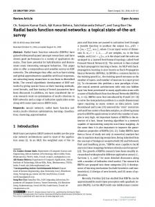
study transmission was made through the vector elements: if that element or node ≥ 𝜆, where 𝜆 = 0.8, else transmission was done by more than one node. It also shows where a decision needs to be taken. For example, whether the same message should be sent twice by a node or be sent by two nodes on the network. It describes the success rate from each node to the sink(s): in most practical applications, more than one sink is used, and sink node is either through the fiber or TTE connection. Figure 9 shows the optimised error and survival probability for one run as follows: CRBF = 0.001173, SBF = 0.01917, and GRBF = 0.0185. At rock hardness of 90% the survival probability was between 73 and 85%. In view of this the AP heads had to be positioned at areas where the rock is relatively soft. In addition, scalability of CRBF model to SBF and GRBF in relations to survival probability range was comparable. Robot location and rock type with their survival probability ranges are displayed in Table 2. The survival probability range also indicated its scalability at various robot locations, different sizes of sensor nodes, and

at different types of rock softness/hardness. The proposed model CRBF competed favourably and better in some cases compared to the SBF and GRBF. The CPU time, memory allocated, and memory at peak period were generated by profiling during Matlab simulation and the details recorded after 10 runs for each model. The relationship between the CPU time, memory allocated, and memory at peak usage with respect to CRBF, SBF, and GRBF was expressed in a second-order polynomial given as 𝑌𝑟 = 𝛽3 𝑋12 + 𝛽2 𝑋1 + 𝛽6 ,

(29)

where 𝑋1 is time, 𝛽 is the coefficient of the polynomial, and the results were displayed in Table 3 and Figure 10. The CPU time recorded was 622.548 for CRBF, 698.722 for SBF, and 753.082 for GRBF. Comparing the three models the second(2nd-) order polynomial was used for the analysis for CPU time. Memory allocation and memory used are better even with increase in sensor nodes. Other parameters assessed were the mean iteration, standard variance, standard deviation, and the convergence time. 3000 nodes divided into 300 nodes per simulation were performed for CRBF and SBF and GRBF. From Tables 4, 5, and 6, the standard variance for the CRBF of 32.52592 was more consistent with the dataset as compared to 33.14 for the SBF which was more dispersed. Similarly, the time the particles took to converge in CRBF (92.5 seconds) was shorter than that of SBF (101.9 seconds) and GRBF (104 seconds). On the other hand the mean


11

Table 4: Average performance in various parameters of compact radial basis function (CRBF) with a target error of 0.01. Runs 1 2 3 4 5 6 7 8 9 10 Total Average Min/max

Mean Iter 17.380 22.960 19.460 19.180 37.900 23.400 21.480 12.240 26.600 18.120 218.720 21.872 25.660 Good

Std Var 21.592 50.090 22.083 35.493 56.349 36.314 33.289 10.255 38.128 21.668 325.259 32.526 46.094 Good

Std Dev 0.044 0.043 0.042 0.043 0.044 0.043 0.044 0.042 0.043 0.044 0.432 0.043 0.002

Conv. time 62.00 125.00 65.00 125.00 125.00 125.00 97.50 20.00 121.50 59.00 925.00 92.50 105.00 Good

F. error 0.008 0.009 0.012 0.01 0.011 0.012 0.015 0.019 0.01 0.008 0.114 0.011 0.011 Good

Good Good Good Good Good Good

Good Good

Table 5: Average performance of various parameters using sigmoid basis function (SBF) with a target error of 0.01. Runs 1 2 3 4 5 6 7 8 9 10 Total AVG Min/max

Mean Iter 17.340 12.220 13.900 27.500 15.580 14.180 14.680 15.000 27.820 17.060 175.280 17.528 15.600 Good

Std Var 35.890 27.710 18.230 57.640 20.850 34.870 20.510 34.420 46.350 34.970 331.440 33.144 39.410 Good

Std Dev 0.031 0.029 0.035 0.034 0.034 0.037 0.035 0.034 0.034 0.035 0.337 0.034 0.008

Conv. time 125.000 100.500 47.000 125.000 68.500 125.000 52.500 125.000 125.000 125.000 1018.500 101.850 78.000

F. error 0.020 0.01 0.011 0.028 0.019 0.012 0.015 0.012 0.020 0.01 0.157 0.016 0.018

Good Good

Good Good Good

Table 6: Average performance of various parameters using Gaussian radial basis function (GRBF) with a target error of 0.01. Runs 1 2 3 4 5 6 7 8 9 10 Total AVG Min/max

MI 29.3 27.04 31.36 29.76 26.32 24.34 24.06 16.34 26.3 27.42 262.240 26.224 15.020

Std Var 40.971 46.691 53.273 51.968 50.596 28.163 27.180 15.905 45.864 42.432 403.043 40.304 37.368 Good

Std Dev 0.0413 0.0439 0.0438 0.0443 0.0443 0.0410 0.0444 0.0444 0.0452 0.0431 0.4357 0.0436 0.004

Conv. time 110.0 125.0 125.0 125.0 125.0 76.0 59.0 45.0 125.0 125.0 1040.00 104.00 80.000

F. error 0.012 0.014 0.021 0.021 0.008 0.009 0.009 0.012 0.014 0.120 0.012 0.013 Good

Good

Good Good Good Good

Optimised error

12

International Journal of Distributed Sensor Networks The structure of SBF, CRBF, and GRBF 1 0.9 0.8 Particles are closer target 0.7 less sensitive to inputs 0.6 conscious on accuracy 0.5 0.4 Particles are far from target sensitive to inputs 0.3 faster 0.2 0.1 0 −10 −8 −6 −4 −2 0 2 4 6 8 10 Particles position SBF CRBF GRBF

Figure 11: The structure of the CRBF, SBF, and GRBF.

iteration of 17.528 and the standard deviation of 0.0337 in SBF showed more favorable results than that of CRBF which was 21.872 and 0.04315 and GRBF’s mean iteration of 26.224 and standard deviation of 0.0436, respectively. In addition

the dataset of CRBF was more consistent than SBF and GRBF, which were more dispersed. From Tables 4–6, the errors of the models were also accessed. The error goal was set at 0.01. The initial and final errors were analysed against the error goal for the same number of simulation in both cases. 60% of the results for RBF had 0.01 as the target set, with 20% having 0.012 (excess of 0.002) and the rest 0.015 and 0.019. However SBF met the target at 30%, with 20% having 0.012 (excess of 0.002), the remaining 50% obtained in excess of the above (0.005). Additionally the performance of the training in terms of the average optimised error was given as 0.011, 0.016, and 0.013 for CRBF, SBF, and GRBF respectively. This also confirms the CRBF superiority over the SBF and GRBF; the RBF’s accurateness over the SBF is also consistent with Hidayat and Ariwahjoedi [49]. From Figure 9 the initial errors of (𝑌 = 0.059), (𝑌 = 0.08), and 0.08 were all reduced after the training to (𝑌 = 0.001173 at point 𝑋 = 249), (𝑌 = 0.0197 at point 𝑋 = 249), and 𝑌 = 0.0185 at point 𝑋 = 249. The results of the general characteristics of the three models with a range of weight set at [−10, 10] are presented in matrix 𝐴, 𝐵, and 𝐶 with the characteristic curves in Figure 11

Columns 1 through 15 −10 − 9 − 8 − 7 − 6 − 5 − 4 − 3 − 2 − 1 0 1 2 3 4 𝐴=( ), Columns 16 through 21 5 6 7 8 9 10 Columns 1 through 9 0.0000 0.0001 0.0003 0.0009 0.0025 0.0067 0.0180 0.0474 0.1192 Columns 10 through 18 ), 𝐵=( 0.2689 0.5000 0.7311 0.8808 0.9526 0.9820 0.9933 0.9975 0.9991 Columns 19 through 21 0.9997 0.9999 1.0000 ( )

(30)

Columns 1 through 9 0.0000 0.0001 0.0003 0.0009 0.0025 0.0067 0.0183 0.0498 0.1353 Columns 10 through 18 ). 𝐶=( 0.3679 1.0000 0.3679 0.1353 0.0498 0.0183 0.0067 0.0025 0.0009 Columns 19 through 21 0.0003 0.0001 0.0000 ( )

The initial stage of the sigmoid function (SBF) grows relatively exponential as 𝑥 touches the 0, and then the growth begins to slow down towards saturation and stops at maturity as 𝑦 goes to 1 (Figure 11). The RBF rises from 0 to 1 and falls as 𝑥 goes to “10.” A combination of both functions, where 𝑥 goes close to negative 4 and intersects the Sigmoid curve at (1, 0.3679), improves the accuracy. Other studies such as velocity-field reconstruction in fluid structure [49] showed the flexibility of the SBF but indicated that the RBF gives better accuracy, attributable to the influence of function parameters. The CRBF and SBF accelerate from the beginning to the peak and decrease as they get closer to the target. However the GRBF lagged a while at 𝑥 = −2 before rising and falling close to 𝑥 = 2 thereby reducing the survival probability range at that point.

9. Conclusion In this study a scale-free wireless sensor routing topology control in 3-dimensional environment for an optimized path in underground mine rescue operation was discussed. Optimization was done numerically using Matlab simulation tool which generated the optimum set of routing table. Through particle swarm algorithm the neural network was trained for rescue operation. Results showed that the combined CRBF with PSO provided better results than SBF and PSO or GRBF and PSO in the neural training. The proposed model was relatively better in terms of scalability and CPU time efficiency. We have also shown that the model is fault tolerant and had a maximum survivability routing path for rescue operations. The model could serve as an alternative in rescue

International Journal of Distributed Sensor Networks operations in the mining sector. We look forward to assess a hybrid of this algorithm with other parameters in future.

Acknowledgments The authors would like to appreciate the immense contribution of the mining companies where the study was undertaken. The authors are grateful to these individuals for their immeasurable contributions to this work: Fred Attakuma, Patrick Addai, Isaac Owusu Kwankye, Thomas Kwaw Annan, Willet Agongo, Nathaniel Quansah, Francis Owusu Mensah, Clement Owusu-Asamoah, Joseph Adu-Mensah, Shadrack Aidoo, Martin Anokye, F. T. Oduro, Ernest Ekow Abano, and E. Omari-Siaw. This work was supported by the National Natural Science Foundation of China (no. 71271103) and by the Six Talents Peak Foundation of Jiangsu Province.

References [1] Editorial Team, “The 3rd issue of volume 12,” Editorial Team, the 3rd issue of volume 12, Disaster Prevention and Management, September 2012, http://www.emeraldinsight.com/ products/journals/journals.htm?id=dpm. [2] G. Hilson, C. J. Hilson, and S. Pardie, “Improving awareness of mercury pollution in small-scale gold mining communities: challenges and ways forward in rural Ghana,” Environmental Research, vol. 103, no. 2, pp. 275–287, 2007. [3] S. S¸alap, M. O. Karslioˇglu, and N. Demirel, “Development of a GIS-based monitoring and management system for underground coal mining safety,” International Journal of Coal Geology, vol. 80, no. 2, pp. 105–112, 2009. [4] N. Amegbey, C. Ampong, and S. Ndur, “Water Pollution from mining in Prestea, Ghana,” in Proceedings of the 3rd International Conference on Environmental Issues and Waste Management in Energy and Mineral Production, pp. 179–184, Western Australia, 1994. [5] H. Kucuker, “Occupational fatalities among coal mine workers in Zonguldak, Turkey, 1994–2003,” Occupational Medicine, vol. 56, no. 2, pp. 144–146, 2006. [6] J. H. Saleh and A. M. Cummings, “Safety in the mining industry and the unfinished legacy of mining accidents: safety levers and defense-in-depth for addressing mining hazards,” Safety Science, vol. 49, no. 6, pp. 764–777, 2011. [7] S. Mainardi, “Earnings and work accident risk: a panel data analysis on mining,” Resources Policy, vol. 30, no. 3, pp. 156–167, 2005. [8] C. M. Coetzee and C. J. van Staden, “Disclosure responses to mining accidents: South African evidence,” Accounting Forum, vol. 35, no. 4, pp. 232–246, 2011. [9] A. R. Silva and M. C. Vuran, “Development of a testbed for wireless underground sensor networks,” EURASIP Journal on Wireless Communications and Networking, vol. 2010, Article ID 620307, 2010. [10] Y. Gu and T. He, “Bounding communication delay in energy harvesting sensor networks,” in Proceedings of the 30th IEEE International Conference on Distributed Computing Systems (ICDCS ’10), pp. 837–847, IEEE Computer Society, June 2010. [11] D. Wu, L. Bao, and R. Li, “A holistic approach to wireless sensor network routing in underground tunnel environments,” Computer Communications, vol. 33, no. 13, pp. 1566–1573, 2010.

13 [12] J. Heidemann, W. Ye, J. Wills, A. Syed, and Y. Li, “Research challenges and applications for underwater sensor networking,” in Proceedings of IEEE Wireless Communications and Networking Conference (WCNC ’06), pp. 228–235, April 2006. [13] S. Vupputuri, K. K. Rachuri, and C. Siva Ram Murthy, “Using mobile data collectors to improve network lifetime of wireless sensor networks with reliability constraints,” Journal of Parallel and Distributed Computing, vol. 70, no. 7, pp. 767–778, 2010. [14] N. Edalat, “Resource management and task allocation in energy harvesting sensor networks.,” in Proceedings of IEEE International Symposium on a World of Wireless, Mobile and Multimedia Networks (WoWMoM ’12), San Francisco, Calif, USA, 2012. [15] D. Niyato, M. M. Rashid, and V. K. Bhargava, “Wireless sensor networks with energy harvesting technologies: a game-theoretic approach to optimal energy management,” IEEE Wireless Communications, vol. 14, no. 4, pp. 90–96, 2007. [16] M. C. Vuran and I. F. Akyildiz, “Channel model and analysis for wireless underground sensor networks in soil medium,” Physical Communication, vol. 3, no. 4, pp. 245–254, 2010. [17] N. Meratnia, B. J. van der Zwaag, H. W. van Dijk, D. J. A. Bijwaard, and P. J. M. Havinga, “Sensor networks in the low lands,” Sensors, vol. 10, no. 9, pp. 8504–8525, 2010. [18] S. L. Goh and D. P. Mandic, “An augmented CRTRL for complex-valued recurrent neural networks,” Neural Networks, vol. 20, no. 10, pp. 1061–1066, 2007. [19] S. Li and F. Qin, “A dynamic neural network approach for solving nonlinear inequalities defined on a graph and its application to distributed, routing-free, range-free localization of WSNs,” Neurocomputing, vol. 117, pp. 72–80, 2013. [20] S. Li, Z. Wang, and Y. Li, “Using laplacian eigenmap as heuristic information to solve nonlinear constraints defined on a graph and its application in distributed range-free localization of wireless sensor networks,” Neural Processing Letters, vol. 37, pp. 411–424, 2013. [21] S. Li, B. Liu, B. Chen, and Y. Lou, “Neural network based mobile phone localization using Bluetooth connectivity,” Neural Computing and Applications, pp. 1–9, 2012. [22] L. A. B. Munoz and J. J. V. Ramosy, “Similarity-based heterogeneous neural networks,” Engineering Letters, vol. 14, no. 2, EL14-2-13, 2007, (Advance online publication: 16 May 2007) . [23] F. Fernández-Navarro, C. Hervás-Mart´ınez, P. A. Gutiérrez, J. M. Peña-Barragán, and F. López-Granados, “Parameter estimation of q-Gaussian radial basis functions neural networks with a hybrid algorithm for binary classification,” Neurocomputing, vol. 75, pp. 123–134, 2012. [24] K. Leblebicioglu and U. Halici, “Infinite dimensional radial basis function neural networks for nonlinear transformations on function spaces,” Nonlinear Analysis: Theory, Methods and Applications, vol. 30, no. 3, pp. 1649–1654, 1997. [25] F. Fernández-Navarro, C. Hervás-Mart´ınez, J. Sanchez-Monedero, and P. A. Gutiérrez, “MELM-GRBF: a modified version of the extreme learning machine for generalized radial basis function neural networks,” Neurocomputing, vol. 74, no. 16, pp. 2502– 2510, 2011. [26] S. Li, S. Chen, B. Liu, Y. Li, and Y. Liang, “Decentralized kinematic control of a class of collaborative redundant manipulators via recurrent neural networks,” Neurocomputing, vol. 91, pp. 1– 10, 2012. [27] S. Li, H. Cui, Y. Li, B. Liu, and Y. Lou, “Decentralized control of collaborative redundant manipulators with partial command

14

[28]

[29]

[30]

[31]

[32]

[33]

[34]

[35]

[36]

[37]

[38]

[39]

[40]

[41] [42] [43]

[44]

[45]

International Journal of Distributed Sensor Networks coverage via locally connected recurrent neural networks,” Neural Computing and Application, 2012. A.-L. Barabási, R. Albert, and H. Jeong, “Mean-field theory for scale-free random networks,” Physica A, vol. 272, no. 1, pp. 173– 187, 1999. S.-H. Yook, H. Jeong, and A.-L. Barabási, “Modeling the internet’s large-scale topology,” Proceedings of the National Academy of Sciences of the United States of America, vol. 99, no. 21, pp. 13382–13386, 2002. K. Akkaya and M. Younis, “A survey on routing protocols for wireless sensor networks,” Ad Hoc Networks, vol. 3, no. 3, pp. 325–349, 2005. S. Zarifzadeh, A. Nayyeri, and N. Yazdani, “Efficient construction of network topology to conserve energy in wireless ad hoc networks,” Computer Communications, vol. 31, no. 1, pp. 160– 173, 2008. Q. Ling, Y. Fu, and Z. Tian, “Localized sensor management for multi-target tracking in wireless sensor networks,” Information Fusion, vol. 12, no. 3, pp. 194–201, 2011. Y. Chen, C.-N. Chuah, and Q. Zhao, “Network configuration for optimal utilization efficiency of wireless sensor networks,” Ad Hoc Networks, vol. 6, no. 1, pp. 92–107, 2008. R. Riaz, A. Naureen, A. Akram, A. H. Akbar, K.-H. Kim, and H. Farooq Ahmed, “A unified security framework with three key management schemes for wireless sensor networks,” Computer Communications, vol. 31, no. 18, pp. 4269–4280, 2008. X. Feng, Z. Xiao, and X. Cui, “Improved RSSI algorithm for wireless sensor networks in 3D,” Journal of Computational Information Systems, vol. 7, no. 16, pp. 5866–5873, 2011. W.-S. Jang, W. M. Healy, and M. J. Skibniewski, “Wireless sensor networks as part of a web-based building environmental monitoring system,” Automation in Construction, vol. 17, no. 6, pp. 729–736, 2008. J. Peng and C. P. Y. Pan, “Particle swarm optimization RBF for gas emission prediction,” Journal of Safety Science and Technology, vol. 11, pp. 77–85, 2011. P. S. Sausen, M. A. Spohn, and A. Perkusich, “Broadcast routing in wireless sensor networks with dynamic power management and multi-coverage backbones,” Information Sciences, vol. 180, no. 5, pp. 653–663, 2010. T. M. Jamel and B. M. Khammas, “Implementation of a sigmoid activation function for neural network using FPGA,” in Proceedings of the 13th Scientific Conference of Al-Ma’moon University College, Baghdad, Iraq, 2012. P. S. Rajpal, K. S. Shishodia, and G. S. Sekhon, “An artificial neural network for modeling reliability, availability and maintainability of a repairable system,” Reliability Engineering and System Safety, vol. 91, no. 7, pp. 809–819, 2006. W. Duch and N. Jankowski, “Survey of neural transfer functions,” Neural Comping Surveys, vol. 2, pp. 163–212, 1999. H. H. Zhang, M. Genton, and P. Liu, “Compactly supported radial basis function kernels,” 2004. J. Kennedy and R. Eberhart, “Particle swarm optimization,’ in Proceedings of IEEE International Conference on Neural Networks, pp. 1942–1948, December 1995. R. C. Eberhart and Y. Shi, “Particle swarm optimization: developments, applications and resources,” in Proceedings of the Congress on Evolutionary Computation, vol. 1, pp. 81–86, May 2001. R. Malhotra and A. Negi, “Reliability modeling using particle swarm optimization,” International Journal of Systems Assurance Engineering and Management, 2013.

[46] D. Gies and Y. Rahmat-Samii, “Particle swarm optimization for reconfigurable phase-differentiated array design,” Microwave and Optical Technology Letters, vol. 38, no. 3, pp. 168–175, 2003. [47] J.-Y. Kim, H.-S. Lee, and J.-H. Park, “A modified particle swarm optimization for optimal power flow,” Journal of Electrical Engineering & Technology, vol. 2, no. 4, pp. 413–419, 2007. [48] A. Alfi, “PSO with adaptive mutation and inertia weight and its application in parameter estimation of dynamic systems,” Acta Automatica Sinica, vol. 37, no. 5, pp. 541–549, 2011. [49] M. I. P. Hidayat and B. Ariwahjoedi, “Model of neural networks with sigmoid and radial basis functions for velocity-field reconstruction in fluid-structure interaction problem,” Journal of Applied Sciences, vol. 11, no. 9, pp. 1587–1593, 2011.

International Journal of

Rotating Machinery

The Scientific World Journal Hindawi Publishing Corporation http://www.hindawi.com

Volume 2014

Engineering Journal of

Hindawi Publishing Corporation http://www.hindawi.com

Volume 2014


Volume 2014

Advances in

Mechanical Engineering

Journal of

Sensors Hindawi Publishing Corporation http://www.hindawi.com

Volume 2014


Distributed Sensor Networks Hindawi Publishing Corporation http://www.hindawi.com


Volume 2014

Advances in

Civil Engineering Hindawi Publishing Corporation http://www.hindawi.com

Volume 2014

Volume 2014

Submit your manuscripts at http://www.hindawi.com

Advances in OptoElectronics

Journal of

Robotics Hindawi Publishing Corporation http://www.hindawi.com


Volume 2014

Volume 2014

VLSI Design

Modelling & Simulation in Engineering


Navigation and Observation


Chemical Engineering Hindawi Publishing Corporation http://www.hindawi.com

Volume 2014



Volume 2014


Advances in

Acoustics and Vibration Volume 2014


Volume 2014

Volume 2014

Journal of

Control Science and Engineering

Active and Passive Electronic Components Hindawi Publishing Corporation http://www.hindawi.com

Volume 2014


Journal of

Antennas and Propagation Hindawi Publishing Corporation http://www.hindawi.com

Shock and Vibration Volume 2014


Volume 2014


Volume 2014

Electrical and Computer Engineering Hindawi Publishing Corporation http://www.hindawi.com

Volume 2014