making sales data analysis and optimizing the sales. Radial. Basis Function neural networks are widely used for classification problems with multi-class ...
International Journal of Computer Applications (0975 – 8887) Volume 26– No.6, July 2011
Radial Basis Function Neural Classifier using a Novel Kernel Density Algorithm for Automobile Sales Data Classification M. Safish Mary
Assistant Professor Department of Computer Science St. Xavier's College (Autonomous) Palayamkottai
ABSTRACT
This paper presents a novel approach for classifying the sales data using neural networks, whose result may be helpful in making sales data analysis and optimizing the sales. Radial Basis Function neural networks are widely used for classification problems with multi-class attributes because of their gradient-descent feature. Our objective is to classify the sales data into three classes: high sales items, moderate sales items and poor sales items. The proposed work is to design an efficient algorithm to classify the data for further analysis. The algorithm must take less time to construct a data classifier with an optimized parameter setting to find the center of the classes there by performing an efficient classification.
Keywords
Classification, Gradient-descent, optimization, Radial Basis Function (RBF), sales data analysis.
1. INTRODUCTION
In finance and business analysis, classification of large volumes of available data is crucial. But this process is time consuming and very complex that analysts always use some automation tools for this classification task. Neural Networks are a proven, widely used technology for solving such complex classification of data. Neural Networks are interconnected networks of independent processors termed as neurons that can be trained to classify any type of data that is given as input. A radial basis function neural network is a special type of neural network commonly used for classification, regression, function approximation and data clustering problems. It uses radial basis function as its activation function [1]. Since its introduction, it has been used widely in many classification problems. The RBFs are characterized by their localization and Gaussian activation function using supervised (gradient based) procedures to obtain the expected result [2]. In a supervised application, the network is provided with a set of input data to be classified called as training samples for which the expected class label is known. After training the classifier till it correctly classifies the input samples, it is tested with another set of data samples called test data, to check the efficiency of the classifier in classifying the given data.
Dr. V. Joseph Raj
Head, Department of Computer Science Kamaraj College, Manonmaniam Sundaranar University, Thoothukudi in poor classification. If the number is too high, poor generalization or an over learning situation occurs [3]. Hence it is very important to determine the number of neurons in the hidden layer to improve the efficiency of the RBF network. The training procedure of RBF networks also includes the optimization of spread parameters of each neuron. Afterwards, the weights between the hidden layer and the output layer must be selected appropriately. Finally, the bias to be added to each output is determined during the training process. In this paper, we have used Radial Basis Function (RBF) network to classify the sales data obtained from a departmental store. The samples are grouped into two sets: one for training the network and the other set for testing the learning capability of the network. The data is classified into three classes as high sales products, moderate sales products and poor sales products. This classification can be used to analyze the sales and make a decision in the purchase of items to the store. This paper is structured as follow: in section 2 the network topology is explained, Section 3 details the training algorithm used for classification, section 4 discusses the experimental results of the study and section 5 gives the concluding remarks.
2. RADIAL BASIS FUNCTION NETWORKS
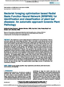
A RBF neural network consists of three layers, namely the input layer, the hidden layer and the output layer. The input layer takes in the coordinates of the input vector to each unit in the hidden layer. Each unit in the hidden layer then produces an activation using the radial basis function used in the layer. Finally, each unit of the hidden layer computes a linear combination of the activations and produces a classified output in the output layer units. The output is entirely based on the use of the activation function used in the hidden layer and the weights associated with the links between the hidden layer and the output layer.
In RBF networks, the number of neurons in the hidden layer affects the network complexity and the generalizing capability of the network. If the number of the neurons in the hidden layer is insufficient, the RBF network cannot learn the data and results
1
International Journal of Computer Applications (0975 – 8887) Volume 26– No.6, July 2011 ii) the average time complexity for classifying m incoming objects is O(m log n)
Radial basis function Weights
∑
O/P 1
iii) the network is able to classify data into more than two classes of objects in one single run.
O/P 2
A data reduction mechanism must be employed to remove redundant samples in the training data set in order to improve the efficiency of the classifier.
O/P q
3. OVERVIEW OF THE PROPOSED LEARNING ALGORITHM
I/P 1 ∑ I/P p
∑
Figure 1: Radial Basis Function Neural Network Architecture Many learning algorithms have been proposed for RBF neural networks depending on the problem for which it is applied [4, 5, 6, 7, 8, 9]. The optimization criteria used will differ depending on the proposed learning algorithm and the problem for which RBF is used. One of the main applications of RBF is data classification. Most learning algorithms determines the number of units in the hidden layer, the activation functions associated with the hidden units and the weights associated with the links between the hidden and output layers. The general mathematical form of the output units in RBF network is as follows: h
f j ( x) wi , j ri ( x) i 1
where
fj
is the function corresponding to the j-th output unit
and is a linear combination of h radial basis functions r1, r2, ………, rh. In the literature, various algorithms are proposed for training RBF networks, such as gradient descent algorithm and Kalman filtering algorithm [8]. These algorithms suffer from the problem of converging to a local minima and finding the optimal gradient is time-consuming. To overcome these limitations several global optimization methods such as genetic algorithms, particle swarm optimization algorithm [9], the artificial immune algorithm [10] and the differential evolution algorithm [11] have been used for training RBF networks for different optimization problems. In this paper, a novel learning algorithm for data classification is presented. In the RBF networks constructed with the proposed learning algorithm, each activation function associated with the hidden units is a spherical or symmetrical Gaussian function. The main properties of the proposed learning algorithm are i) the average time complexity for constructing the network is O(n log n), where n is the total number of training samples;
This section explains the algorithm that has been used for classifying the data into the required classes. Each training sample is given to the network as an input. The learning algorithm places one spherical Gaussian function at each training sample. The general form of the Spherical Gaussian Function network based function approximations is as follows:
ˆf v w exp v si i 2 2 j siS j i
2
where (i) (ii) (iii) (iv) (v)
is the spherical Gaussian function approximator for class-j training samples; v is the input vector; Sj is the set of class-j training samples; is the distance between vectors v and si wi and σi are parameters to be set by the learning algorithm.
With the spherical Gaussian function, a new class located at v is predicted to belong to the class with the maximum value of the likelihood function defined in the following equation:
L j (v )
Sj S
fˆ j (v)
Where Sj is the set of class-j training samples and S is the set of training samples of all classes. We can estimate the value of the probability density function at a class-j sample si as follows: m (k1 1) R( si ) m 2 f j ( si ) m Sj ( 1) 2
1
2
International Journal of Computer Applications (0975 – 8887) Volume 26– No.6, July 2011 where (i)
R(si) is the maximum distance between si and its k1 nearest training samples of the same class.
(ii)
is the volume of a hyper sphere with
number of hidden layer neurons to be used in the neural network for the specified problem. The obtained sales data was preprocessed to remove noise and redundant attributes and attributes with wide range of unique values was normalized Table 1: Classification accuracy of original data and preprocessed data using SGF neural network
radius R(si) (iii) is the Gaussian approximation function (iv) K1 is a parameter to be set either through cross validation or by the user. For a training sample si , the learning algorithm first conducts a mathematical analysis on a synthesized data set. The challenge is how to figure out the optimal wi and σi values of each Gaussian function. By repeated training the optimal value for σi is obtained using the formula
i
where
R ( si ) m m ( k 1) ( 1) 1 2
. Different values of β will give different
smoothing effects.
wi
(k1 1) (
m 1) 2
m S j R ( s i ) m
Training Accuracy (%)
Testing Accuracy (%)
Execution Time
Full Data (420*3)
89.7
85.6
3 hrs
Processed Data (240*3)
91
90
2.9sec
Reduced Data (100*3)
92.3
92.1
2.7 sec
The neural network performed at its best and the percentage of correct classification was above 91%. The network was trained with different centers and also by varying the initial spread value and the smoothing ratio β.
5. CONCLUSION m 2
Where
h2 exp 2 h 2
The first issue to be addressed is the time taken to create a Spherical Gaussian Function for the neural network with n training samples and the second issue is the time taken to classify m objects with the proposed network.
4. EXPERIMENTAL STUDY
The data used for this study was collected from a local automobile dealer. There were 700 records i.e., sales records from year 2008 to 2010. The proposed neural network was trained to classify the input records into high sales automobiles, moderate sales item and poorly sold cars. Out of the 700 samples, 420 samples (60%) were used for training the network and the remaining 40% samples were used as the test data. There is a critical implementation issue in the representation of the class information as part of the input. Feature selection is a critical process in any classification task which determines the
The results of this study can be used for predicting the automobile buying pattern among the customers, to analyze the sales trend of the automobiles, and finalize the demand requirements of the customers. Also more attributes can be included so that the sales impact due to the location of the customers, any sales promotions and marketing strategies can be studied effectively. For an efficient and effective implementation of this research, data from more than one automobile dealer must be collected for a sufficient period of time and comparing the performance of the neural network for larger number of records. The classification results can be analyzed by combining some fuzzy models which can effectively predict the results accurately [12]. In future research the results of this study can be compared with the performance of SVM and particle swarm optimization methods.
6. REFERENCES
[1] M. J. L. Orr, 1996 Introduction to radial basis function networks, Technical report, Center for Cognitive Science, University of Edinburgh. [2] Karayiannis, N, 1997 Gradient descent learning of radial basis neural networks, Proc. of the IEEE International Conference on Neural Networks, Houston, TX, pp. 18251830. [3] Liu, Y: Zheng, Q.; Shi, Z.; Chen, J. 2004 Training radial basis function networks with particle swarms, Computer Science, 3173.
3
International Journal of Computer Applications (0975 – 8887) Volume 26– No.6, July 2011 [4] Karayiannis, N.B., 1999 Reformulated radial basis neural networks trained by gradient descent, IEEE Transactions on Neural Networks, 3, 2230–2235
[9] Liu, Y.; Zheng, Q.; Shi, Z.; Chen, J., 2004 Training radial basis function networks with particle swarms, Lecture Notes Computer Science, 3173, 317–322.
[5] C. Harpham et al., 2004 A review of genetic algorithms applied to training radial basis function networks, Neural Computing and Applications 13(3), 193-201.
[10] De Castro, L. N.; Von Zuben, F.J., 2001 An immunological Approach to Initialize centers of Radial Basis Function Neural Networks, In Proceedings of Brazilian Conference on Neural Networks, Rio de Janeiro, Brazil,; pp. 79-84.
[6] Du, J.X.; Zhai, C.M., 2008 A hybrid learning algorithm combined with generalized approach for radial basis function neural networks, Applied Mathematical Computing, 208, 908–915. [7] Oyang, Y.J.; Hwang, S.C.; Ou, Y.Y.; Chen, C.Y.; Chen, Z.W., 2005 Data classification with radial basis function networks based on a novel kernel density estimation algorithm, IEEE Transactions on Neural Networks, 16, 225–236.
[11] Yu, B; He, X., 2006 Training Radial Basis Function Networks with Differential Evolution, In Proceedings of IEEE International Conference on Granular Computing, Atlanta, GA, USA, 369-372. [12] Pei-Chann Chang; Yen-Wen Wang; Chi-Yang Tsai, Evolving Neural Network for printed circuit board sales forecasting, Expert Systems with Applications, vol. 29, Issue 1, pg: 83-92
[8] Simon, D., 2002 Training radial basis neural networks with the extended Kalman filter, Neurocomputing, 48, 455–475.
4