distributions of ionizing radiation in tissue equivalent gels infused with ... We have investigated the diffusion problem in Fricke gel dosimetry using finite-element.
Phys. Med. Biol. 41 (1996) 1745–1753. Printed in the UK
A method for determining the diffusion coefficient in Fe(II/III) radiation dosimetry gels using finite elements P J Harris†, A Piercy† and C Baldock‡ † Department of Mathematical Sciences, University of Brighton, Lewes Road, Brighton, UK ‡ Department of Medical Physics, Royal Sussex County Hospital, Eastern Road, Brighton, UK Received 1 February 1996, in final form 1 April 1996 Abstract. Magnetic resonance imaging (MRI) may be used to image three-dimensional dose distributions of ionizing radiation in tissue equivalent gels infused with ferrous sulphate solutions, commonly known as Fricke gels. In this technique, ferrous (Fe2+ ) ions are oxidized to ferric (Fe3+ ) ions by free radicals produced by ionizing radiation. A limitation on this technique is the diffussion of ferric (Fe3+ ) ions in the gel. A method is presented for evaluating the diffusion coefficient in Fricke gels. Finite elements are used to model variations of the concentration in space, coupled with an analytical scheme to integrate the resulting system of equations through time. This method may be used for problems with one, two or three space dimensions and with arbitrary initial and boundary conditions. Results are presented for one- and two-dimensional data.
1. Introduction It was demonstrated in 1984 (Gore et al 1984) that magnetic resonance imaging (MRI) may be used to image three-dimensional dose distributions of ionizing radiation in tissue equivalent gels infused with ferrous sulphate solutions. The gels are commonly known as Fricke gels. In this technique, ferrous (Fe2+ ) ions are oxidized to ferric (Fe3+ ) ions by free radicals produced by ionizing radiation and the increased paramagnetic enhancement of the waterproton relaxation rates, due to the presence of the ferric ions, is imaged using MRI. MRI dosimetry with Fricke gels has generated a number of publications (Appleby et al 1988, Baldock et al 1995, Balcom et al 1995, Day 1990, Gambarini et al 1994, Hazle et al 1991, Kron et al 1993, Kron and Pope 1994, Olsson et al 1989, 1990, 1992b, Podgorsak and Schreiner 1990, Prasad et al 1991, Rousseau et al 1994, Schulz et al 1990). A limitation on the measurement technique in Fricke gel dosimetry is the diffussion of ferric ions in the gel (Balcom et al 1995, Olsson et al 1992a, Schulz et al 1990) and alternative formulations of gels based on polymers which exhibit no diffusion have been investigated (Baldock et al 1996, Maryanski et al 1993, 1994). Fricke gels, however, retain some practical advantages and continue to be of interest particularly if the signal diffusion can be calculated in routine applications. We have investigated the diffusion problem in Fricke gel dosimetry using finite-element numerical methods. With the appropriate choice of boundary conditions, the resulting coupled system of differential equations may be analytically solved to determine the diffusion coefficient from experimental data. A number of methods have been proposed for finding the diffusion coefficient (see Asakura et al 1991, Balcom et al 1993, 1995, 0031-9155/96/091745+09$19.50
c 1996 IOP Publishing Ltd
1745
1746
P J Harris et al
Guillot et al 1991, Pearl et al 1991 for instance). However, these methods are often appropriate only for situations which involve only one space dimension and a particular initial dose distribution. The method described here can be applied to one, two or three space dimensions for any initial and final dose distribution. 2. Numerical methods For simplicity, we illustrate the method for a problem with one space dimension. The concentration U is given by @ 2U @U =µ 2 (1) @t @x where µ is the diffusion coefficient. This section will introduce a finite-element method for discretizing equation (1) in space and then analytically integrating the resulting system of coupled linear ordinary differential equations through time. The finite-element method was chosen since it can readily deal with non-equally spaced data, and in two or three dimensions it can accommodate irregular shaped domains. A further advantage of choosing the finite-element method is that the analysis of the time integration scheme is the same regardless of the number of space dimensions. Consider equation (1) defined on some interval [a, b] of the real line, with initial condition U (x, 0) = U0 (x) and boundary condition @U/@x which is known at the two end points of the interval. The solution is approximated by n X u(x, t) = uj (t) j (x). (2) j =1
This solution is assumed to satisfy the boundary conditions. Replacing the exact solution U (x, t) in the differential equation (1) by the approximate solution u(x, t) yields the residual function @ 2u @u µ 2. (3) r(x, t) = @t @x The finite-element method now requires that the residual is orthogonal to each of the basis functions i . That is Z b r(x, t) i (x) dx = 0 i = 1, 2, . . . , n. (4) a
This condition ensures that, for any given value of t, r(x, t) cannot be expressed as a linear combination of the basis functions j (x) and consequently r(x, t) will be ‘small’. Substituting (3) into (4) yields Z b 2 Z b @u @ u dx. (5) i dx = µ 2 i @t @x a a Evaluating the integral on the right-hand side of (5) using the parts rule yields ✓ ◆ Z b Z b @u @u @u d i @u (b) i (b) (a) i (a) + µ dx. (6) i dx = µ @x @x @x dx a @t a Substituting in (2), the definition of the approximate solution, and since the approximate solution is assumed to satisfy the boundary conditions, it follows that ✓ ◆ Z Z b n n X X duj b d jd i @U @U uj (b) i (b) (a) i (a) + µ dx (7) j i dx = µ dt a @x @x dx dx a j =1 j =1
Determining diffusion coefficient in Fricke gels
1747
for i = 1, 2, . . . , n. This can be written in matrix notation as Mu ˙ = µKu + µf
(8)
˙ = (du1 /dt, . . . , dun /dt)T and where u = (u1 (t), u2 (t), . . . , un (t))T , u Z b Mij = i j dx a
Z
b d id j dx Kij = a dx dx ◆ ✓ @U @U (b) i (b) (a) i (a) f= @x @x
(9)
(note the use of an over-dot to denote differentiation with respect to time). The matrix K is usually referred to as the stiffness matrix and the matrix M as the mass matrix, by analogy with mechanical vibration problems. Although it is possible to use high-order polynomials over the whole interval as the basis functions i this is hardly ever done in practice. The finite-element method divides the region R into a number of small sub-intervals (called elements). The points at which the elements join together are called the node points. Each node has a basis function associated with it, which is defined to be zero in any element not containing the node and a simple low-order polynomial, such as linear or quadratic, over the elements which contain the node. This reduces the amount of work needed to compute the matrices in (9) above as most of the entries will be zero. For problems involving two or three space dimensions, the analysis is similar to the one-dimensional case above and yields a matrix equation of the same form as (8). Details of finite-element methods in two or three dimensions can be found in one of the many specialized texts available, such as that by Zienkiewicz and Taylor (1989). The matrix equation (8) can now be considered as a system of coupled first-order linear differential equations, which can be integrated through time using the analytical techniques described below. This analytical time integration scheme was chosen since it has the advantage that once the eigenvalues and eigenvectors have been computed it is possible to find the finite-element solution for different end times, different initial conditions and different boundary conditions relatively quickly. Re-arranging the matrix equation (8) yields u ˙ = µM
1
Ku + µM
1
f.
(10)
It can be shown that the mass matrix will always be non-singular provided the basis functions i are linearly independent. It is a well known result from linear algebra that it is possible to express the matrix M 1 K in the form M
1
1
K = P DP
(11)
where D is a diagonal matrix. It is relatively easy to show that the elements of D are just the eigenvalues of M 1 K and the columns of P are the corresponding eigenvectors. Substituting (11) into (10) and re-arranging yields u + µP
1
Making the change of variables w = P
1
P
1
u ˙ = µDP
1
w ˙ = µDw + µg
M
1
f.
(12)
u gives the uncoupled system of equations (13)
1748
P J Harris et al
where g = P
1
M
1
f . Alternatively, this can be written as
w˙ 1 = µ 1 w1 + µg1 w˙ 2 = µ 2 w2 + µg2 ...
w˙ n = µ n wn + µgn
(14)
where 1 , 2 , . . . , n are the eigenvalues of the matrix M 1 K. The solution to each of the equations in (14) can be written in the form Z t wi (t) = eµ i t wi (0) + µ eµ i t e µ i T gi (T ) dT . (15) 0
Thus
w(t) = E(t)w(0) + F (t)
(16)
where E(t) is a diagonal matrix with elements Eii (t) = eµ
it
and Fi (t) = µeµ
it
(17) Z
t
e
µ iT
gi (T ) dT .
(18)
0
Writing the solution w in term of the original variables u gives the finite-element solution to the diffusion equation as 1
u(t) = P E(t)P
u(0) + P F (t)
(19)
where u(0) is found by simply evaluating the initial condition U0 (x) at the node-points. For certain simple boundary conditions it is possible to carry out the integration in the definition of F analytically (see (18)). In such cases it is possible to obtain a simple matrix expression for the solution at time t in terms of the initial condtions and the boundary conditions. In terms of the vector f appearing in (10) Z t e µ i T P 1 M 1 f i dT (20) Fi (t) = µ eµ i t 0
where P 1 M 1 f i denotes the ith component of P 1 M independent of time then Z t µ it 1 1 Fi (t) = µ e e µ i T dT P M f i
1
f . If the components of f are
(21)
0
and evaluating the integral yields 8✓ µ t ◆ i 1 > < e (P Fi (t) = i > : µt (P 1 M 1 f )i
1
M
1
f )i
i
6= 0
i
= 0.
(22)
It should be noted at this point that since all the boundary conditions are in terms of @u/@n there will always be at least one zero eigenvalue. It follows that if the boundary conditions do not vary with time F (t) = G(t)P
1
M
1
f
(23)
Determining diffusion coefficient in Fricke gels where G(t) is a diagonal matrix with elements 8✓ ◆ µ it 1 > < e Gii (t) = i > : µt
i
6= 0
i
= 0.
1749
(24)
In this case the finite-element solution to the diffusion equation can be written as u(t) = P E(t)P
1
u(0) + P G(t)P
1
M
1
f.
(25)
For cases where the boundary conditions do depend on time it may be necessary to evaluate the integral appearing in (20) numerically. The eigenvalues and eigenvectors of the matrix M 1 K can be computed directly, or more appropriately by solving the generalized eigenvalue problem Kx = Mx as this avoids the need to directly invert the mass matrix M. Once these have been found it is possible to compute the approximate solution to (1) for times t > 0 using (25). 3. Determination of the diffusion coefficient The numerical model outlined above can used to determine the diffusion coefficient from experimental data. Suppose v(0) is the experimental distribution at time t = 0 and v(T ) is the distribution at some later time T . It is assumed that v(0) and v(T ) are known at a set of points which correspond to the nodes of a finite-element mesh. By taking u(0) = v(0) it is possible to compute u(T ) using (25) (assuming that the boundary conditions are in a suitable form) for a given value of the diffusion parameter µ . The error between the computed solution and the experimental distribution can be defined as err =
n X (vi (T )
ui (T ))2 .
(26)
i=1
The required value of µ is then the one which minimizes the error. There are a number of numerical methods for finding the optimal value of µ which minimizes the error. In the present work the required value of µ was found using the following simple binary search. Suppose the required value is known to lie in some interval [µa , µb ]. The error err is computed at the three points µ1 = µa + h/4, µ2 = µa + h/2 and µ3 = µa + 3h/4 where h = µb µa . If the error is smallest at µ1 then the new interval is taken as [µa , µ2 ] . Similarly if the error at µ2 is smallest then the new interval is [µ1 , µ3 ] whilst if the error at µ3 is smallest the new interval is [µ2 , µb ]. In each case the error has already been found at the mid-point of the new interval so it is only necessary to compute the error at the 1/4 and 3/4 points of the new interval. This process of reducing the length of the interval is continued until the length of the interval containing the required value of µ is smaller than some pre-determined tolerence. The mid-point of the final interval is taken as the location of the required value of µ. 4. Results This section presents the results of using the model introduced in sections 2 and 3 for computing the diffusion coefficient for a number of one- and two-dimensional test problems. The test problems were generated by assuming some initial condition ue (0) and fixed value of the diffusion constant µe with boundary conditions dU/dn = 0. The ‘exact’ solution ue (T ) was then computed using (25). The simulated experimental data v(0) and v(T )
1750
P J Harris et al
were formed by introducing a range of random errors into ue (0) and ue (T ). The diffusion coefficient was then determined from these data using the methods described in the previous sections. Figure 1 shows the results of the determination of the diffusion coefficient by fitting to some randomized data. Here ‘Initial’ is used to denote the simulated initial concentration profile with random errors, ‘Final’ to denote the simulated final concentration profile with random errors and ‘Fitted’ to denote the concentration profile obtained using (21) with the optimized value of the diffusion coefficient. The induced errors in the initial and final profiles were uniformally distributed between prescribed limits of ±5%. The original value of µ was 0.02 and the fitted value obtained was 0.019 88.
Figure 1. The initial, final and fitted concentrations for a typical test problem.
Figure 2 gives the percentage relative error in the fitted value of the diffusion coefficient for different maximum errors in the initial and final concentrations, where the errors are either uniformly or approximately normally distributed. The results are given for oneand two-dimensional problems and are, in each case, the mean of 100 different initial and final concentrations with the given maximum errors. Figure 3 gives the corresponding root-mean-square differences between fitted final concentrations u(T ) and the actual final concentrations v(T ). As expected, as the errors in the original data increase, so do the errors in the fitted value of the diffusion coefficient and between the ‘Final’ and ‘Fitted’ profiles. However, the results show that, even with relatively large errors in the orginal data, this method manages to determine the diffusion coefficient to within ±10%. We note that the errors in the results for the two-dimensional problem are consistently smaller than the corresponding errors in the results for the one-dimensional problem. Finally, this method was applied to the measured concentrations obtained from three samples of gel stored for known times at room temperature. The fitted values of the diffusion coefficient were 0.020 896, 0.021 346 and 0.023 499. These values are consistent with the results of previous experiments, as described elsewhere (see Baldock et al 1995).
Determining diffusion coefficient in Fricke gels
1751
Figure 2. The percentage relative error in the diffusion coefficient for different maximum errors in the input data.
Figure 3. The root-mean-square error in the fitted model for different errors in the input data.
5. Conclusions This paper has shown how the finite-element method can be used to compute the diffusion coefficient from some experimental data. The numerical results for the test problem have shown that this method yields a reasonable estimate of the diffusion coefficient even when there are relatively large errors in the data used. When used with real data obtained from a MRI experiment this method gives values of the diffusion coefficient which agree with
1752
P J Harris et al
values obtained in previous studies. However, this method has the advantage that it can be applied to any initial and final distribution of the concentration and can be easily adapted for problems with two or three space dimensions. The methods described in this paper may also be applied to the problem of compensating for the effects of diffusion in clinical applications of the Fricke gel technique. This is possible by specifying negative times in equation (25) to determine the dose distribution at the time of irradiation.
References Appleby A, Leghrouz A and Christman E A 1988 Radiation chemical and magnetic resonance studies of aqueous agarose gels containing ferrous ions Radiat. Phys. Chem. 32 241–4 Asakura T, Demura M, Ogawa H, Matsushita K and Imanari M 1991 NMR imaging of diffusion of small organic molecules in silk fibrion gel Macromolecules 24, 620–2 Balcom B J, Fischer A E, Carpenter T A and Hall L D 1993 Diffusion in aqueous gels. Mutual diffusion coefficients measured by one-dimensional nuclear magnetic resonance imaging. J. Am. Chem. Soc. 115 3300–5 Balcom B J, Lees T J, Sharp A R, Kulkarn N S amd Wagner G S 1995 Diffusion in Fe(II/III) radiation dosimetry gels measured by magnetic resonance imaging Phys. Med. Biol. 40 1665–76 Baldock C, Burford R P, Billingham N C, Cohen D and Keevil S F 1996 Polymer gel composition in magnetic resonance dosimetry Proc. Int. Soc. Magn. Reson. Med. (New York, 1996) pp 1594 Baldock C, Harris P J, Piercy A R, Patval S, Prior D N, Keevil S F and Summers P 1995 Temperature dependence of diffusion in Fricke gel MRI dosimetry. 37th Scientific Meeting of American Association of Physicists in Medicine, Boston, July 1995 Med. Phys. 22 1540–1 Day M J 1990 Radiation dosimetry using nuclear magnetic resonance: an introductory review Phys. Med. Biol. 35 1605–9 Gambarini G, Arrigoni S, Cantone M C, Moiho N, Facchielli L and Sichirollo A E 1994. Dose-response curve slope improvement and result reproducibility of ferrous-sulphate-doped gels analysed by NMR imaging Phys. Med. Biol. 39 703–17 Gore J C, Kang Y S and Shulz R J 1984 Measurements of radiation dose distributions by nuclear magnetic resonance imaging Phys. Med. Biol. 29 1189–97 Guillot G, Kassab G, Hulin J P and Rigord P J 1991 Monitoring of tracer dispersion in porous media by NMR imaging J. Phys. D: Appl. Phys. 24 763–73 Hazle J D, Hefner L, Nyerick C E, Wilson L and Boyer A L 1991 Dose-response characteristics of a ferrous sulphate doped gelatin system for determining radiation absorbed dose distributions by magnetic resonance imaging (Fe MRI) Phys. Med. Biol. 36 1117–25 Kron T, Metcalfe P and Pope J M 1993 Investigation of the tissue equivalence of gels used for NMR dosimetry Phys. Med. Biol. 38 139–50 Kron T and Pope J M 1994 Dose distribution measurements in superficial X-ray beams using NMR dosimetry Phys. Med. Biol. 39 1337–49 Maryanski M J, Gore J C, Kennan R P and Schulz R J 1993 NMR relaxation enhancement in gels polymerised and cross-linked by ionizing radiation: a new approach to 3-D dosimetry. Magn. Reson. Imaging 11 253–8 Maryanski M J, Schulz R J, Ibbott G S, Gatenbury J C, Xie J, Horton D and Gore J C 1994 Magnetic resonance imaging of radiation dose distributions using a polymer gel dosimeter Phys. Med. Biol. 39 1437–55 Olsson L E, Arndt J and Fransson A 1992b Three dimensional dose mapping from gamma knife treatment using a dosimeter gel and MR imaging. Radiother. Oncol. 24 8286 Olsson L E, Fransson A, Ericsson A and Mattsson S 1990 MR imaging of absorbed dose distributions for radiotherapy using ferrous sulphate gels Phys. Med. Biol. 35 1623–31 Olsson L E, Peterson S, Ahlgern L and Mattsson S 1989 Ferrous sulphate gels for determination of absorbed dose distributions using MRI technique: basic studies Phys. Med. Biol. 34 43–52 Olsson L E, Westrin B, Fransson A and Nordell B 1992a Diffusion of ferric ions in agarose dosimeter gels Phys. Med. Biol. 37 2243–3352 Pearl Z, Magaritz M and Bendel P J 1991 Measuring diffusion coefficients of solutes in porous media by NMR imaging J. Magn. Reson. 95 597–602 Podgorsak M B and Schreiner L J 1990 Nuclear magnetic relaxation characterisation of irradiated Fricke solution Med. Phys. 19 87–95
Determining diffusion coefficient in Fricke gels
1753
Prasad P V, Nalcioglu O and Rabbini B 1991 Measurement of three dimensional radiation dose distribution using MRI Radiat. Res. 128 1–13 Rousseau J, Gibbon D, Sarrazin T, Doukhan N and Marchandise X 1994 Magnetic resonance imaging of agarose gel phantom for assessment of three-dimensional dose distribution in linac radiosurgery Br. J. Radiol. 67 646–8 Schulz R J, de Guzman A F, Nguyen D B and Gore J C 1990 Dose-response curves for Fricke infused agarose gels as obtained by nuclear magnetic resonance Phys. Med. Biol. 35 1611–22 Zienkiewicz O C and Taylor R L 1989 The Finite Element 4th edn, vols 1 and 2 (London: McGraw-Hill)