I. Kožar, D. Lozzi-Kožar
Određivanje gustoće toka konačnim elementima: globalni naspram lokalnog izračuna ISSN 1330-3651 (Print), ISSN 1848-6339 (Online) DOI: 10.17559/TV-20160208123711
FLUX DETERMINATION USING FINITE ELEMENTS: GLOBAL VS. LOCAL CALCULATION Ivica Kožar, Danila Lozzi-Kožar Original scientific paper Finite difference procedures for flux determination are not well suited for application to field results obtained from finite element calculations. A novel method for flux calculation has been derived. This method is based on the weak formulation and is suitable for use with finite elements. A matrix formulation for local and global application to finite element formulations is presented. An additional benefit of the method is that Neumann boundary conditions can be easily incorporated in the finite element formulation of the nonlinear field problem. A comparison between the finite difference, Pade derivative and novel finite element procedures is demonstrated through one- and two-dimensional examples. Keywords: boundary condition; finite element; flux determination; matrix formulation; nonlinear field problem; weak formulation
Određivanje gustoće toka konačnim elementima: globalni naspram lokalnog izračuna Izvorni znanstveni članak Metoda konačnih razlika nije prikladna za određivanje gustoće toka polja izračunatog metodom konačnih elemenata. Načinjena je nova metoda za računanje gustoće toka koja se temelji na slaboj formulaciji i prikladna je za upotrebu s konačnim elementima. Prikazana je matrična formulacija za lokalnu i globalnu primjenu u metodi konačnih elemenata. Dodatna prednost metode je da se Neumann-ov rubni uvjet lako može ugraditi u formulaciju konačnih elemenata kojom se opisuje nelinearni problem rješavanja polja. Na jedno- i dvo- dimenzionalnim primjerima prikazuje se usporedba rješenja metodom konačnih razlika, Pade-ove derivacije i nove metode s konačnim elementima. Ključne riječi: gustoća toka; konačni element; matrična formulacija; nelinearni problem izračuna polja; rubni uvjet; slaba formulacija
1
Introduction
Many numerical fluid flow and heat transfer problems encounter the problem of determining flux from known field results. In this paper, we attempt to present a broader picture of the flux determination procedure. Traditionally, this problem is considered secondary to the problem of field determination, a consequence of a logical attempt to reduce the problem as much as possible. Typically, one solves for the scalar field (temperature, concentration, etc.), and flux is found from the result using some derivation procedure. The derivation procedure is usually performed using a finite difference scheme, regardless of the method used for domain discretization (finite elements (FE) [1], finite differences (FD) [2] or finite volumes (FV) [3]). The main advantage of finite difference schemes in their explicit (local) forms is that they are calculated quickly and do not require inversion. As in [2] and [4], some combinations of discretization methods for field and derivative calculations result in poor performance. Among these, unfortunately, is the combinations of finite elements and finite differences, and much effort has been applied to investigating improved schemes. One improvement involves transforming the local finite difference formulation into a global, higher order difference scheme that includes the entire domain in a derivative calculation, such as the Pade scheme [5]. Another adopted approach is the "super convergent patch recovery", which is based on an extrapolation of field results and a solution of the minimum squares problem [4]. Both approaches require inversion, that is, the solution of an additional system of equations that incorporates part or all of the domain of the problem. The determination of derivatives can be part of the original problem; that is, the field equation and flux (derivative) equation are coupled, though weakly. Only in the case of Dirichlet boundary conditions is this weak coupling resolved, allowing equations to be solved Tehnički vjesnik 24, 1(2017), 247-252
consecutively. In the case of Neumann boundary conditions, the derivative equation should be treated as a constraint of the field equation. Otherwise, equations can be solved consecutively, as with the Dirichlet boundary condition; but the Neumann condition is only approximately fulfilled as a result. This coupling is always present in inverse problems unless the conductivity coefficient is constant. Moreover, due to stability requirements, high accuracy is required in inverse problems, motivating this work [6]. Herein, the field equation and the flux (derivative) equation are both rewritten in their weak forms. This approach allows the same finite element discretization to be applied to both equations; that is, the weak form of the field equation is extended to the accompanying derivative equation. Both explicit and implicit procedures can be devised. The explicit procedure is a result of applying the Galerkin weak formulation to the finite element level, and the derivative is calculated element-wise. The implicit procedure results when this weak formulation is applied to the entire structure, that is, when the element matrices are assembled into a global derivative matrix. Application of the same discretization and calculation procedure to both field and derivative quantities results in a much more precise result. A similar benefit is shown in [7], with a procedure developed for curvilinear finite elements. Based on the weak formulation, this work presents a novel procedure for the calculation of flux and other derivative-dependent quantities for finite elements. The procedure is suitable for all types of finite elements. Throughout the paper, matrix formulation is favoured. The method will be illustrated using 1D and 2D examples of flux calculations for heat transfer. 2
Strong form of equations
The primary equation of the nonlinear field problem is the partial differential equation of the form
247
Flux determination using finite elements: global vs. local calculation
∇(k (ξ ))T = R
I. Kožar, D. Lozzi-Kožar
(1)
where T stands for temperature filed values and R stands for the right hand vector that contains the boundary conditions (or source/sink terms) and ξ is replaced with either x for space dependency or with T for temperature dependency. The secondary equation for calculating the derivative value (flux) is
q = k ( x)
d T dxt
(2)
which is in the form of a differential equation, although it is not acknowledged as such because the right hand side is considered known (the field, T, is calculated from the primary Eq. (1)). k is the vector of known (except in inverse problems) thermal conductivity coefficients. Whether Eqs. (1) and (2) are coupled depends on the boundary conditions, i.e. for Dirichlet boundary condition Eq. (1) is self-contained since R is expressed in terms of T only; for Neumann boundary condition R is expressed in terms of k and Eqs. (1) and (2) are coupled. Whether Eq. (2) is explicit or implicit depends on whether the flux is calculated locally or globally. Local flux calculation is flux calculation in one node only from known field values from the surrounding nodes, like in finite difference method. In this case q is expressed explicitly. Global flux calculation is the one where flux is calculated in all the nodes simultaneously and q is a function of all the field nodal values. In this case q cannot be expressed in explicit form and cannot be calculated directly. An example of such a problem is the Pade derivative formulation. In most cases, the equations are uncoupled; that is, the strong form is resolved by solving the primary Eq. (1), and its derivative (flux) is calculated (explicitly or implicitly) from the known field T using the secondary Eq. (2). We shall assume that the numerical procedure uses matrix differentiation operators [5], i.e. differentiation of a vector is performed by multiplying the vector with a specially prepared "differentiation matrix". From Eq. (1), the matrix formulation for finite differences lists
T =[D[diag(k ) D ]]−1 ⋅R
(3a)
where D is a differentiation matrix. Only in the case of finite differences vector of conductivity coefficients k can be extracted from the differentiation matrix D as a separate diagonal matrix. Further, for finite volumes we have
T =[K V (k )]−1 ⋅ R
(3b)
and for finite elements we write
T =[K E(k e )]−1 ⋅ R
(3c)
where KV and KE are differentiation matrices corresponding to the desired differentiation method and are functions of conductivity coefficient vector k. The 248
exponent "−1" stands for matrix inversion but, in practice, refers to the solution of a system of linear equations. There is a difference between vectors k and ke, vector k represents the nodal values of conductivity coefficients, and ke represents the finite element average of the nodal values; simple interchange of k and ke leads to erroneous result. Matrix KE is constructed differently in classical versus novel finite element formulations, as will be shown later. From Eqs. (2) and (3a), the flux can be expressed as
q = [diag(k )]D ⋅ T
(4a)
for finite differences. For explicit q formulation in finite volumes and "classical" finite elements the formulation is similar. For implicit q formulation and the novel finite element procedure we can write q = DE (k e ) −1 ⋅ T
(4b)
Different forms of differentiation operators can be applied in Eqs. (3) to (4). In [8] there is an example of application using a spectral differentiation operator. In most cases, lower order finite differences are applied, and Eq. (4a) is explicit, as stated. If greater accuracy is needed, higher derivative terms should be included. In this paper, the Pade derivation scheme has been considered an example of a differential operator with very high accuracy. However, flux equation is no longer explicit because, in the Pade formulation, the flux is derived from the equation
DP ( k ) ⋅ q = d P ⋅ T
or
q = DP (k ) −1 ⋅ d P ⋅ T .
(4c)
where dP and DP are vector and matrix operator [5]. In this paper those operators have been combined into single matrix derivation operator so Eq. (4c) takes the form of Eq. (4b). Index P stands for a ‘Pade’ finite difference scheme. Eq. (4b) is used throughout the examples for the comparison of flux values derived from different methods. It should be noted that the Galerkin formulation in its weak form takes form of Eq. (4b) that corresponds to the Pade formulation in its strong form, Eq. (4c). They are both local with regard to neighbouring points (arbitrary number of surrounding nodes are included) and global with regard to the domain (nodal values in the whole domain are related), leading to implicit forms that require solution of the resulting system of linear equations. It is immediately evident that in the case of finite element model, the correct flux value cannot be derived from Eq. (4a) or (4c) based on the temperature obtained from Eq. (3c) because they do not incorporate element value ke and simple interchange of k and ke leads to erroneous result; equation of the type of Eq. (4b) is required. However, the required Eq. (4b) has not been found in the literature, and its use is considered a novel approach. 3
Weak form of the flux equation
An approach consistent with the finite element method would require the weak formulation of the Technical Gazette 24, 1(2017), 247-252
I. Kožar, D. Lozzi-Kožar
Određivanje gustoće toka konačnim elementima: globalni naspram lokalnog izračuna
derivative problem, necessitating that Eq. (2) is entirely transformed into its integral form. Instead of solving directly Eq. (2), it is necessary to solve its weak form, obtained by applying the Galerkin procedure to the diffusive part and the flux part separately
Now, global equation assembled over all the elements
is
(e)
(e)
or
dN ( x) ∫ N ( x)q( x) − k ( x) dx T ( x) dx = 0
(5a)
(e)
(e)
(C (e) q (e) ) = ( R (e)T (e) ) ⇒ ∑ C (e) q = ∑ R (e) T Cq = RT .
(8)
As on the element level matrix C is symmetric, nonsingular and positive-definite so
We can write the above equation on the finite element level,
q = C −1 RT
dN ke N V .E . dx
which is the same as in [9]. Moreover, if we form a matrix Λ on the element and global (assembled) level
∫
T dx TE = NN dx q E V .E .
∫
(5b)
where N is a vector of element shape functions, and ke, qE, TE are vectors pertaining to the finite element method. Upon choosing a finite element type and solving the integrals (analytically or numerically) the resulting matrix equation is Dq ⋅ q = D E ( k e ) ⋅ T C
(e) ( e)
q
(e)
=R T
(5c)
(e)
(5d)
which resolves into Eq. (4b). Eqs. (5) and, consequently, Eq. (4b) can be formulated locally (on the level of one finite element) or globally (assembled elements). 4
Relation to the conjugated space formulation
It can be shown that equations (5) are related to the conjugate finite element space [9]. The following notation in [9] we write
T
(9)
T
Λe = C e N T , ΛT = C −1 N T then (with Ω = ∑ (e) )
∫N
−1 Λ d(e) = ∫ N T N C (e) d(e) = (e)
T
(e)
=
C (e)
(6)
(e)
where (e) means element domain and C is symmetric, non-singular and positive-definite matrix. We assemble elements over the whole domain
C=
C (e) and
R=
∫N
T
∫
(7)
(e)
(e)
Ω
(.)
operates differently on finite element matrices and differently on nodal vectors: while element components are summed (i.e. (k (1) , k (3) ) = K (1) + K (3) etc.), nodal
vector components are forming a real union (i.e. (1) ( X (3) , X (3) ) = X (3) ( X (1) , X (3) ) = X (3) and X etc.) since they are in the domain space. Here K(e) is a finite element matrix transformed into the (global) domain space (i.e. K (e ) = T T k (e )T where T is a local to global transformation matrix). Tehnički vjesnik 24, 1(2017), 247-252
( )
∫
Ω
−1
Ω
= (C )(C ) = I
(12)
and ( e)T
∫Λ
Λ( e) d(e) =
∫C
( e ) −1
T
−1
N ( e) N ( e) C ( e) d(e) =
(e)
−1 −1 T = C ( e) ∫ N ( e) N ( e) d(e) C ( e) = ( e )
(13)
−1 −1 −1 = C ( e) C ( e) C (e) =C (e)
∫Λ
T
∫
Λ dΩ = C −1N T NC −1dΩ = Ω
( )∫ N N dΩ (C ) = C C (C ) = C
= C −1
T
−1
−1
−1
−1
(14)
Ω
It is important to note that the union operator
( )
Λ dΩ = N T N C −1 dΩ = N T N dΩ C −1 =
Ω
R (e)
(11)
( )
T ( e ) ( e ) −1 (e) −1 ∫ N N d(e) C = C C = I (e)
( e)
∂N = ∫ N T N d(e) and R e = ∫ k (e ) N T d(e) ∂x (e) (e)
(10)
as in [9] but on both, the element and assembled levels. We can conclude that on the global level (all elements assembled) this formulation is equivalent to the formulation in conjugated space with all the advantages and disadvantages (continuity over element boundaries that results in very accurate flux values, lack of local support that requires solution of the resulting system of linear equations). However, the great advantage is formulation in the form of a finite element that permits easy incorporation into existing codes, use of the existing finite element mesh and formation of element patches of arbitrary size (and arbitrary accuracy).
249
Flux determination using finite elements: global vs. local calculation
The novel flux calculation method presented in this paper will be explained using the nonlinear heat diffusion equation as an example, but the method is generally applicable. Additionally, there will be a comparison to finite difference and finite volume methods. Solution of the nonlinear heat diffusion equation depends on the heat conduction coefficient ‘k’ (Eq. (2)), which can be either temperature-dependent (k=k(T), as in example 2) or position-dependent (k=k(x), as in example 1). The constant ‘k’ is trivial because the heat equation is linear, Eqs. (1) and (2) are uncoupled and the temperature field distribution is smooth. In that case the difference between methods is not pronounced and will not be addressed in the paper. The problem with flux that arises with the use of the finite element model is especially clear in cases where the flux ‘q’ fluctuates or is given as the Neumann boundary condition (i.e., must be constant, with ‘k’ being variable, etc.). The case of fluctuating (non-physical) ‘q’ in the eddy diffusivity problem was the main motivation for this work [6]. 5.1 Example 1 As an introduction to the problem, numerical results will be calculated and compared for a 1D diffusion problem with arbitrarily varying ‘k’ and constrained ‘q’=const. (due to simplicity and the availability of an analytical result). Such a ‘k’ can result from an inverse problem [6]. Flux is calculated from the temperature field using Eq. (2), and the analytical solution (adapted from [10]) is ΔT q= L . In this problem, ‘k’ is distributed 1 dx k ( x) 0
∫
−k 0 ⋅ r , with a 1 + exp − x ⋅ a + s k0=0,05 W/m2K, r=0,9, a=20 and s=2. Parameters of the (non-physical) diffusion coefficient have been determined by applying the inverse method on the measured temperature distribution in Lake Botonega in Istria, Croatia [6]. The discretized k is distributed as shown in Fig. 1. to
k ( x) = k 0 +
FE analytical FV FD
0.5
0
0
2
4
6
8
10
12
14
16
18
20
position (discretized)
Figure 2 Temperature distribution according to various solution procedures
The maximum error in FE is less than 2 %; in FD, 2,3 %; and in FV, 2,2 %. The flux is calculated according to Eq. (4). Only the novel FE procedure gives the correct (constant) flux result. Note that the novel procedure uses the temperature result from the FE calculation, while FD and Pade use analytical temperature values (providing less accurate numerical results). Errors in the flux results are shown in Fig. 3. The maximum error using the Pade procedure was less than 0,2 %. 0.2 FE FD Pade
0 − 0.2
0
2
4
6
8
10
12
14
16
18
20
position (discretized)
Figure 3 Error in flux distribution using various calculation procedures
5.2 Example 2 This example concerns the diffusion coefficient as a function of temperature k=k(T) and is adapted from [11]. There is a linear dependence on the temperature, k(T)=a(T+1), which results in a nonlinear space dependence that, in general, cannot be calculated in advance because it depends on the temperature field. The boundary conditions are Dirichlet on both ends, and a=0,1. The calculation procedure is iterative, and the flux results after the first iteration for three methods – finite differences, finite volumes and finite elements – are shown in Fig. 4.
0.04 0.14
0.02 0
new FE FD Pade from analytical
0.12
0
5
10
15
20
position (discretized)
Figure 1 Distribution of the (non-physical) diffusion parameter
For a temperature difference ∆T=1,0, the analytical flux value is qT=0,0112006 W/m2. The boundary condition is of Dirichlet type (T0=0,0 K) on the left end and of Neumann type on the right end (qn=0,0112006 250
1
flux
diffusion parameter
according
W/m2). The domain of L=1,0 m is divided into 20 points and discretized using FD, FV and FE. For the purpose of the flux calculation, the derivative matrices have been constructed based on FD, the Pade method, and the novel finite element procedure (Eq. (3) and Eq. (4)). Temperature results are given in Fig. 2.
temperature
Numerical examples
error [1/1000]
5
I. Kožar, D. Lozzi-Kožar
0.1 0.08 0
2
4
6
8
10
12
14
16
18
20
position (discretized)
Figure 4 Flux distribution after the first iteration using different flux calculation methods
The analytical solution is valid for the first iteration only; it changes as the temperature distribution changes Technical Gazette 24, 1(2017), 247-252
I. Kožar, D. Lozzi-Kožar
Određivanje gustoće toka konačnim elementima: globalni naspram lokalnog izračuna
(because the problem requires an iterative solution procedure). This example converges quickly, and after 5 iterations, the temperature results from the previous and current iterations are equal to 9 digits for all three methods. Five iterations are needed for FV and FD to converge properly, while FE requires fewer iterations. Fig. 5 shows the flux results obtained using different methods.
scheme represents the most accurate finite difference procedure for calculation of derivatives. 1
y
0.5
0
0
0.5
1
x
flux
0.2
new FE FD Pade from analytical
0.15
0.1
0
2
8
6
4
10
12
14
16
18
20
position (discretized)
Figure 5 Flux distribution from converged temperature distribution after 5 iterations using different flux calculation methods
−3
diff.coefficient
2×10
FD FV FE FV-FD FE-FD
0.15
0.1
0
2
4
6
8
10
12
14
16
18
− 2×10
−3
differenece in diff.coef.
0.2
Figure 7 The finite element mesh used in the example and the resulting temperature distribution
20
position (discretized)
Figure 6 Differences in converged diffusion after 5 iterations for different calculation methods
The diffusion coefficient has converged as well and is no longer linear in coordinate space (of course, it is always linear in the temperature space). Fig. 6 shows the converged diffusion coefficients (left ordinate axis) and differences among those calculated using FV and FE (right ordinate axis) in comparison with those from FD. It is interesting to note that results from FV are not smooth. From Figs. 4, 5, and 6, one can conclude that the novel FE flux calculation method demonstrates superior behaviour. 5.3 Example 3
Tehnički vjesnik 24, 1(2017), 247-252
Figure 8 Flux produced by the novel FE method (left) and by the Pade derivative (right), after averaging − 0.01
flux
The third example is a 2-dimensional version of example 1 and uses triangular CST elements for discretization. The problem is homogeneous in the y direction, so plate width should not be important (in practice, the finite element discretization dictates the solution homogeneity in the y direction). The mesh is intentionally unsymmetrical, as this is the unfavourable situation. Figure 7 shows the temperature distribution that corresponds to that from Fig. 2 (taking into consideration the low number of elements). The flux is calculated using the Pade and novel FE schemes; the FD results are much worse and have not been compared. It is well known that nodal results in CST elements should be averaged for optimal accuracy [4], and Fig. 8 compares the two procedures. For illustration, Fig. 9 compares the fluxes resulting from the application of the Pade and novel FE schemes before nodal averaging. It should be noted that the Pade
− 0.012
− 0.014
Pade novel FE 1
2
3
4
5
6
position (discretixed)
Figure 9 Un-averaged flux comparison along the edge
251
Flux determination using finite elements: global vs. local calculation
It is evident from Figs. 8 and 9 that the novel FE method in two dimensions also has superior capabilities related to flux determination. 6
Conclusion
This paper presents a novel procedure for flux calculation derived from the weak formulation and is suitable for finite element applications. Based on a matrix formulation, modified finite elements have been constructed and demonstrated using example applications of a two node line element for 1D problems and a three node CST element for 2D problem. The examples provide a comparison of flux calculation results obtained using new method and the typical Pade differentiating procedure. Examples feature 1D and 2D problems with position- and temperature-dependent heat diffusion coefficients. The superiority and broad applicability of the novel finite element procedure has been clearly demonstrated. Nomenclature dq – matrix used in the novel finite element procedure k – diffusion parameter (non-physical in examples) k(x) – position dependent diffusion parameter k(T) – temperature dependent diffusion parameter k – discretized diffusion parameter q – flux q – discretized flux T – temperature T – discretized temperature field D – derivation matrix (for the relevant discretization method) KV, KE – system matrix for the finite volume method, for the finite element method N – finite element shape function
I. Kožar, D. Lozzi-Kožar
Part B: Fundamentals: An International Journal of Computation and Methodology. 22, 2(1992), pp. 243-250. [8] Kožar, I.; Torić Malić, N. Spectral method in realistic modelling of bridges under moving vehicles. // Engineering Structures. 50, (2013), pp. 149-157. DOI: 10.1016/j.engstruct.2012.10.024 [9] Oden, J. T.; Brauchli, H. I. On the Calculation of Consistent Stress Distributions in Finite Element Approximations. // International Journal for Numerical Methods in Engineering. 3, 3(1971), pp. 317-325. DOI: 10.1002/nme.1620030303 [10] Hens, H. Building Physics – Heat, Air and Moisture. Ernst & Sohn, A Wiley Company, 2007. [11] Chang, C.-L.; Chang, M. Inverse determination of thermal conductivity using semi-discretization method. // Applied Mathematical Modelling. 33, 2(2009), pp. 1644-1655. DOI: 10.1016/j.apm.2008.03.001 Authors’ addresses Ivica Kožar, PhD, Full Prof. University of Rijeka, Faculty of Civil Engineering, Department for Computer Modeling, Radmile Matejcic 3, 51000 Rijeka, Croatia E-mail:
[email protected] Danila Lozzi-Kožar, PhD Croatian Waters, Djure Sporera 3, 51000 Rijeka, Croatia E-mail:
[email protected]
Acknowledgements This paper has been partially funded through Croatian Science Foundation project 9068: Multi-scale concrete model with parameter identification, which is fully appreciated. 7
References
[1] Lewis, R. W.; Nithiarasu, P.; Seetharamu, K. N. Fundamentals of the Finite Element Method for Heat and Fluid Flow. 2nd ed. Chichester : Wiley, 2005. [2] Ferziger, J.H.; Peric, M. Computational Methods for Fluid Dynamics. Springer, 2001. [3] Versteeg, H. K.; Malalasekera, W. Computational Fluid Dynamics. The Finite Volume Method. 2nd ed. Essex : Pearson Prantice Hall, 2007. [4] Akin, J. E. Finite Element Analysis with Error Estimators. Oxford : Elsevier Butterworth-Heinemann, 2005. [5] Moin, P. Fundamentals of Engineering Numerical Analysis. 2nd ed. New York : Cambridge University Press, 2007. [6] Lozzi-Kožar, D. Three-dimensional Modeling of Thermal Distribution in Lake "Botonega". (in Croatian), Ph.D. Thesis, The University of Split, Split, Croatia, 2012. [7] Shai, I.; Szanto, M.; Anteby, I. Technical Note: Numerical Heat Flux Calculation in FEM. // Numerical Heat Transfer, 252
Technical Gazette 24, 1(2017), 247-252