the nominal phase of the PRISMA mission provide an opportunity for the
implementation of an ... Keywords: FFRF, GPS, relative navigation, fusion,
PRISMA. 1.
RADIO-FREQUENCY SENSOR FUSION FOR RELATIVE NAVIGATION OF FORMATION FLYING SATELLITES G. Allende-Alba(1), S. D’Amico(2), and O. Montenbruck(2) (1) Institut für Astronomische und Physikalische Geodäsie, Technische Universität München, 80333 München, Germany (2) German Space Operations Center, Deutsches Zentrum für Luft-und Raumfahrt, 82230 Weβling, Germany Abstract: The increasing need for robustness, reliability and flexibility of relative navigation systems imposed by the current and future autonomous formation flying missions, calls for the implementation of solutions using an alternative approach to single-sensor systems. These schemes possess different levels of availability mainly driven by sensor failure and mission orbit profiles. The data obtained from the Global Positioning System (GPS) and Formation Flying Radio-Frequency (FFRF) sensors from the nominal phase of the PRISMA mission provide an opportunity for the implementation of an extended approach for the generation of relative navigation solutions. The present study introduces the design of a simple relative navigation filter based on the sensor fusion concept, which makes use of differential GPS and FFRF measurements obtained from the on-board sensors. The filter design uses the HillClohessy-Wiltshire and Yamanaka-Ankersen relative dynamics models as well as numerical integration methods including the J2-perturbation for the state and associated covariance matrix propagation. The design is tested using flight data obtained during representative formation flying operations of the PRISMA mission. Keywords: FFRF, GPS, relative navigation, fusion, PRISMA. 1. Introduction The use of the GPS for relative navigation of formation flying satellites in Low Earth Orbit (LEO) has achieved a high degree of maturity over the past 15 years, mainly due to the capability of this navigation system of providing the required accuracy and precision for various formation flying profiles, such as rendezvous and interferometric baseline operations [1]. The recent PRISMA mission represents a milestone in the field of formation flying given that it provides an in-orbit test-bed for new sensor and actuators systems. Among these systems, the FFRF sensor represents the first non-GPS RF-based metrology instrument for relative navigation to be flown in an actual mission [2]. The FFRF sensor provides a precise relative navigation solution independent of any GNSS constellation through the generation of its own navigation signals [3]. The GPS and FFRF data obtained from the PRISMA mission provides the opportunity of implementation of an extended approach to single-sensor relative navigation systems. The present study introduces the design of a simple extended Kalman filter for relative navigation, considering the sensor fusion concept and making use of differential GPS and FFRF measurements in order to increase the robustness, reliability and availability of the delivered solution.
2. RF measurements and sensor fusion architecture 2.1. FFRF measurements The FFRF sensor has been derived from the GPS technology and it is capable of producing, for each spacecraft in the formation, relative distance and line of sight (LOS) measurements concerning all its companions. The distance between two satellites is obtained by combining their respective pseudorange measurements in order to remove inter-equipment clock bias and for this purpose navigation data must be exchanged through the inter-satellite link (ISL) provided by the FFRF instrument [3]. The LOS measurements rely on interferometry techniques and they are obtained by measuring the carrier phase difference between two antennas (master and slave) on the triplet antenna base of the FFRF subsystem [2] (see Fig. 1). When both distance and LOS measurements make use of carrier phase in order to achieve the nominal precision, it is necessary to execute additional procedures and algorithms for Integer Ambiguity Resolution (IAR). Such procedures are executed first to solve ambiguity in LOS measurements in order to be able to solve ambiguity on distance. This approach mitigates multipath effects which are direction dependent [3].
Figure 1. PRISMA spacecraft. Mango (left) and Tango (right). (Source: SSC) 2.2. GPS measurements As a result from the diverse system requirements of recent formation flying missions, the GPS technology has been used for the generation of different kind of products for offline and real-time processing. Current approaches for the generation of these products are based on filtering using dynamical models [4], which make them unsuitable for blending with pure kinematic FFRF measurements. Instead, based on the targeted accuracy at the centimeter-level and driven by the mechanical characteristics of FFRF measurements, a single dynamical filtering approach that makes use of purely
kinematic GPS measurements is desirable. For this purpose, the GPS navigation fixes obtained from code measurements are too coarse to be considered and hence a set of more precise measurements is preferred. As an add-on solution to the Precise Orbit Determination (POD) product obtained from the DLR’s GPS High precision Orbit determination Software Tools (GHOST), a purely kinematic relative position solution can be computed from the ambiguity-fixed differential carrier phases [5,6]. Thus, this product is not available for real-time processing but has been provided from offline processing in order to be used for the present study. However, recent research on Precise Point Positioning (PPP) for LEO satellites might provide in the near future similar accuracies to those obtained offline by means of differential GPS techniques [7]. 2.3. Sensor fusion architecture The sensor fusion concept has been considered and successfully applied for several years for terrestrial applications (both military and civilian) where features such as robustness and flexibility are the main drivers. Although not a new concept, the emergence of new sensors, advanced processing techniques and improved processing hardware make data fusion increasingly appealing [8]. This argument can be extended to the case of sensor fusion for relative navigation of formation flying satellites.
Figure 2. FFRF and GPS sensor fusion architecture. Broadening common terminology, the sensor fusion scheme proposed in the present study uses the term track fusion for the merging of estimates from individual sensor tracks whereas the term scan fusion is used for algorithms that combine observations from different sensors [9]. In the context of the proposed design, the FFRF data track provides measurements suitable for scan fusion while the GPS data track results in estimated data, which is adequate for track fusion. Exploiting the features of the available data, the proposed architecture combines these two sources of information in a hybrid scan-track fusion algorithm, as sketched in Fig. 2. The box in dashed line indicates the part of the architecture that was implemented in the present study.
3. Filter design 3.1. Problem description The main objective of the present filter design is the delivery of relative navigation solutions of the deputy (Mango in the PRISMA context) spacecraft’s center of mass with the best possible accuracy (centimeter-level) in the local orbital frame by making use of FFRF and GPS measurements. The local orbital frame (also known as Euler-Hill frame and denoted by ℋ) is referred to the target (Tango in the PRISMA context) spacecraft’s center of mass and constructed out of the radial, tangential (along-track) and normal (cross-track) unit vectors of the target absolute orbit. In order to achieve the centimeterlevel accuracy, the filter has to cope with biases of the FFRF data, which may affect significantly the final relative navigation solution. To this end, the estimated data contained in the filter state vector �, must include the relative state vector (position and velocity) as well as the FFRF float biases. 3.2. Observation and measurement models 3.2.1. GPS sensor The precise kinematic GPS products are provided by GHOST in an Earth-Centered Earth-Fixed (ECEF) reference frame (denoted as ℰ) in the form of absolute position vectors �ℰ for each spacecraft in the formation (Mango and Tango). Thereby, the GPS observation model can be expressed as Δ� ℋ �� = Δ ℋ � = �ℰℋ ��� � ∙ ��ℰ� − �ℰ� � + �� . Δ ℋ
(1)
Here, the rotation matrix �ℰℋ has an explicit dependence to a reference orbit �� which is used to define the ℋ frame and can be generated from the highly-available GPS navigation fixes of the Tango spacecraft. The GPS observation vector �� denotes the relative position of the Mango spacecraft’s center of mass in the ℋ frame (Δ� ℋ , Δ ℋ and Δ ℋ corresponding to radial, along-track and cross-track components, respectively) and is used as a set of (pseudo-)measurements in the filter algorithm. The vector �� represents noise and other unmodeled factors in the GPS observables. In order to include this GPS data set in the fusion filter, it must be assessed so that their statistical properties can be properly reflected in the filtering algorithm. A comparison between precise dynamic and kinematic products provides an indication of the expected errors, as shown in Fig. 3 for a data arc of 50.5 hours. An rms error of 6 mm and 6.7 mm is achieved in the along-track and cross-track components respectively, whereas the radial component exhibits an rms error of 1.5 cm. The slightly worse noise levels in the radial component are a consequence of the bad local vertical geometry of the formation with respect to the GPS constellation.
Radial [m] Along-track [m] Cross-track [m]
0.2
0.003+/-0.015 m
0 -0.2
28-18
28-22
29-02
29-06
29-10
29-14
29-18
29-22
30-02
30-06
30-10
0.2
30-14
30-18
0.001+/-0.006 m
0 -0.2
28-18
28-22
29-02
29-06
29-10
29-14
29-18
29-22
30-02
30-06
30-10
30-14
30-18
0.2 0.002+/-0.007 m
0 -0.2
28-18
28-22
29-02
29-06
29-10 29-14 29-18 29-22 Time UTC [2010/10/dd-HH]
30-02
30-06
30-10
30-14
30-18
Figure 3. Errors in GPS (pseudo-)measurements in the Euler-Hill frame from 2010/10/28-16:00 to 2010/10/30-18:30 UTC with POD as reference. During this data arc, the two spacecraft perform various formation flying operations. Similarly, the form of the vector given by Eq. 1 defines the GPS measurement model � denotes the current estimated filter state vector in to be used in the filter algorithm. If � the filtering algorithm, the GPS measurement model can be expressed as �� � , ℎ � = ℎ � ��
(2)
where the superscript �∙�� denotes the predicted value of the estimated state. 3.2.2. FFRF sensor Once the IAR procedures are executed, the FFRF sensor is designed to deliver measurements denoting the relative position of the phase center of the Tango active antenna expressed in the RF frame (denoted by ℱ). This frame is referred to the phase center of the master Rx/Tx antenna on the Mango spacecraft and axes defined to match the body-fixed frame of the Mango spacecraft [3] (see Fig. 1). The FFRF observation model can be constructed from the computation of the relative distance ! and the LOS measurements in the � and components (�"#$ and "#$ , respectively), as follows (�Δ� ℱ �) + �Δ ℱ �) + �Δ ℱ �) �% = &�"#$ ' = � + + + �, , Δ� ℱ /! "#$ ℱ Δ /! !
(3)
where �% is a vector of FFRF measurements. The vector + represents the cumulated bias affecting the distance and LOS measurements due to residual electrical biases along RF cables, uncertainty on the location of Rx antennas phase center and residual multipath errors [3]. The vector �, represents noise and other unmodeled factors in the FFRF observables.
1
-0.13+/-0.02 m
0 -1
XLOS [deg]
28-18 4 2 0 -2 -4
YLOS [deg]
Distance [m]
As in the case of the GPS data set, in order to include FFRF data in the filtering algorithm, it must be assessed in order to analyze their statistical properties. Figure 4 shows the errors in FFRF measurements expressed in the ℱ frame as defined by Eq. 3. The errors are assessed for a data arc of 50.5 hours using POD products as reference. From the analysis of the FFRF data assessment shown in Fig. 4, it is possible to observe the non-constant bias in LOS measurements, whose fluctuations are attributed to sensor temperature variations [10]. In addition, large angular excursions (in LOS measurements) are present due to multipath effects during attitude maneuvers [11].
4 2 0 -2 -4
28-22
29-02
29-06
29-10
29-14
29-18
29-22
30-02
30-06
30-10
30-14
30-18
0.86+/-0.16 deg
28-18
28-22
29-02
29-06
29-10
29-14
29-18
29-22
30-02
30-06
30-10
30-14
30-18
-0.69+/-0.21 deg
28-18
28-22
29-02
29-06
29-10 29-14 29-18 29-22 30-02 Time UTC [2010/10/dd-HH]
30-06
30-10
30-14
30-18
Figure 4. Errors in FFRF measurements in the RF frame from 2010/10/28-16:00 to 2010/10/30-18:30 UTC with POD as reference. During this data arc, the two spacecraft perform various formation flying operations. According to the proposed filter design, the estimated filter state vector and the FFRF measurements are expressed in different reference frames, which implies that the FFRF measurement model must depend on the attitude quaternions of the Tango and Mango spacecraft ( - � and -� respectively) as well as on the reference orbit �� for the construction of the ℋ frame. In addition, the evaluation of the measurement model in �� . Finally, the navigation filter makes it dependent on the current estimated vector � according to the FFRF sensor design, the distance and LOS measurements are not available at exactly the same times [3], which indicates that two different models can be considered for the filtering algorithm, as follows �� �, -� , - � , �� � ℎ. = ℎ. �! �� 0 � � �, "#$ �� ���, -� , - � , �� � , ℎ = ℎ ��"#$ �� 0
(4a) (4b)
where the dependence of the model on the current predicted filter state vector may not be in general the same for both type of measurements. 3.3. Relative dynamics The filtering algorithm requires the prediction of the state (and its associated error covariance matrix) which in turn is used as a-priori information in the computation of the
updated state. This prediction step is aided from the knowledge of the dynamics of the spacecraft in the formation. Two well-known linear analytical relative dynamics models for unperturbed motion are used in the present design. These are the Hill-ClohessyWiltshire (HCW) model [12,13], suitable for circular reference orbits and the YamanakaAnkersen (YA) model [14], which can be applied for problems with elliptical reference orbits of arbitrary eccentricity. These models are particularly appealing given their simplicity, but they provide only approximations for the case of perturbed motion. In particular, the zonal geopotential coefficient J2 causes one of the largest perturbations for LEO satellites and should be considered in the description of the relative motion of the spacecraft in the formation. Table 1. Relative dynamics strategies for state propagation. State vector propagation
State covariance matrix propagation
Analytical model (Hill-Clohessy-Wiltshire & Yamanaka-Ankersen) Difference of absolute Analytical model states from numerical (Hill-Clohessy-Wiltshire & integration Yamanaka-Ankersen)
A more precise evaluation of the relative dynamics calls for the analysis of orbital perturbations but in order to keep the design as simple as possible (yet accurate) only the J2-perturbation is considered. However, due to the complexity of the analytical equations of perturbed motion, there are no simple implementations of a linearized model1 and the dynamical equations must be integrated numerically. On the other hand, the state error propagation in the filtering algorithm still requires the usage of a linear relative dynamics model. Even though the HCW and YA models are sub-optimal models, their relative simplicity and the provided good approximations for the description of relative motion makes them suitable for propagation of the associated state covariance matrix. Table 1 shows a summary of the different approaches for the relative dynamics of the spacecraft formation flying implemented in the present study. 3.4. Algorithm description 3.4.1. Bias estimation According to the model given by Eq. 3, the FFRF observables are subject to biases that may degrade a relative navigation solution if not coped for. The biases in XLOS and YLOS measurements can be effectively tackled by estimation and previous analyses of the on-board FFRF-based relative navigation filter have demonstrated the feasibility of this approach [10,11]. 1
Existing approaches such as the Gim-Alfriend [15] and Montenbruck-D’Amico [16,17] analytical models require transformations of relative orbital elements, making them unsuitable for the present design, for which simplicity is one of the main goals.
In order to understand how to manage the biases of the FFRF measurements in the filter design, assume for the moment that a set of LOS and distance measurements are available at the same time 12 . Dropping the explicit notation of reference frames for simplicity and denoting the relative state vector as � = 3�, �4 5� , the general observation model of Eq. 3 can be fully written as �% �12 � = 6% �12 ���12 � + 7% �12 �+�12 � + �, �12 � ,
(5)
+�1: � = ;�1: , 1:�< �+�1:�< � + => �1: � .
(6)
where 6% is the linearized version of models shown in Eq. 4 and 8 may take the values ! or 9 (distance and LOS, respectively). The matrix 7% maps the bias vector + into the FFRF measurement vector �% . Similarly, the bias vector can be propagated in time using a general Gauss-Markov model, as follows The measurement noise vector �, and the bias process noise vector => are assumed as Gaussian, zero mean and temporally uncorrelated, with covariance matrices ?% and @> , respectively. The state transition matrix (STM) A of the analytical relative dynamics model can be augmented by considering matrix ; in Eq. 6, as follows B=C
ADED FGED
FDEG H, ;GEG
(7)
with an augmented process noise covariance matrix @. Expressing the filter state vector as � = 3�, +5� , the Gauss-Markov and the general (FFRF) observation models of the system are given respectively by ��1: � = B�1: , 1:�< ���1:�< � + I�1: � + =�1: � �% �12 � = J % �12 ���12 � + �, �12 � ,
(8a) (8b)
where the augmented linearized measurement model is given by J % = 36% 7% 5. The same approach can easily be extended for the case of GPS measurements, where J � = 36� FGEG 5 and 6� is the linearized version of the model given by Eq. 2. Similarly, vector I represents a control input to the system, such as a maneuver burn. Furthermore, according to Eq. 5 and considering independent sets of FFRF distance, FFRF LOS and GPS measurements, the noise covariance of every measurement equation is expressed in the matrices ?. , ?0 and ?� , respectively. 3.4.2. Synchronization of measurements and filtering algorithm One of the main problems that sensor fusion systems face is the non-synchronicity of measurements. This is a natural consequence derived from sensor design and the different sample rates and latencies. However, this situation is not limited to the use of diverse sensors but it can be present even in single-sensor designs. An example of this
is the FFRF instrument, which provides LOS and distance measurements approximately every second but at different times and thus, a synchronization strategy should be considered if the measurements are to be used in a sequential estimation algorithm [3]. In addition when GPS measurements (provided every 10 or 20 seconds for the present study) are incorporated into the filter design, this synchronization strategy must be extended in order to properly manage the timing characteristics of such measurements. Considering the a-synchronicity among LOS and GPS measurements and the nonsequent delivery rate of distance measurements, the present design is focused on the maximal usage of available FFRF measurements generating a relative navigation solution by executing an innovation when a distance or a set of LOS measurements are available. Based on the primary design of the on-board relative navigation filter [3], the delivery rate of the solution can be matched to the LOS measurements latency, but an equivalent approach can easily be obtained by matching the delivery rate to the distance measurement times. The present design has the capability of performing a state propagation by using solely analytical models or by means of a hybrid approach where a numerical integration method is included in the algorithm, as shown in Table 1. As expected, performing a numerical integration (considering the inclusion of J2-perturbation) for state propagation provides more precision but also imposes a higher computational burden. On the other hand, the effective mitigation of some errors caused by the presence of biases in LOS measurements highly relies in the precision of the relative dynamics model. Thus, the selection of the proper approach for state propagation is based on a trade-off between the required precision for a given mission phase and computational burden. State propagation using only an analytical model can be performed by using Eq. 8a, whereas using a hybrid approach requires some extra procedures, as further developed hereafter. Having a filter state vector estimate (along with a set absolute state vectors for both spacecraft) at time 1K a solution can be computed at the execution time 1L if either a set of FFRF LOS or GPS measurements is available. The predicted state is obtained first by performing a numerical integration of the absolute state vectors of the Tango and Mango spacecraft, as follows �ℐ� �ℐ� � � �1L � = 8�1L , 1K ; � � �1K �� ℐ� � � ℐ� � � � � 1L = 8�1L , 1K ; � �� 1K � , �
(9a) (9b)
where the function 8�∙� represents a numerical integrator using the Runge-Kutta 4 method for the two-body problem considering a J2-perturbed motion. The notation ℐ denotes a vector referred to an Earth-Centered Inertial (ECI) reference frame. The obtained absolute orbit of the Tango and Mango spacecraft are used to compute �� , which in turn is projected to the ℋ frame. the a-priori relative state vector Δ� Consequently, the a-priori augmented state vector can be formed by including the ���1L � = 3Δ� ���1L �, +� �1L �5� . propagated biases (according to Eq. 6), as � To complete the time update of the filter algorithm, it is necessary to propagate the error covariance matrix O, associated with the estimated state. Assuming that a matrix OP �1K � is available, the uncertainty of the state can be propagated by using a linearized dynamical model based on a given STM, as shown in Table 1. Considering a bias
propagation matrix ;�1L , 1K � = QGEG , the matrix OP�1K � can be propagated to time 1L using the augmented STM B given by Eq. 7, by means of the Lyapunov equation, as follows O� �1L � = B�1L , 1K �OP �1K �BR �1L , 1K � + @
(10)
< �� �1" �X − !4�1" �T1 − UL �1" , T1�T1 ) !V �1. � = ℎ. W�
(11)
The augmented process noise matrix @ is added to prevent filter divergence and to include the uncertainties in the knowledge of the relative dynamics model into the estimation algorithm. This matrix can be tuned up in order to achieve the best filter performance. ���1L � and its Once the time update provides the a-priori value for the state vector � �� � associated covariance matrix O 1L , the innovation of the algorithm can be computed. At this point, the filter distinguishes between LOS measurements and GPS measurements, namely the execution time 1L = 1" ||1� . When computing the innovation due to LOS measurements (i.e. 1L = 1" ), distance measurements are included in the algorithm by computing an estimate of the relative distance between both spacecraft at time 1. = 1" − T1, where T1 is the delay between both types of measurements. Following [3], the estimated distance at time 1. can be computed by using the measurement model ℎ. , given by Eq. 4a, the distance rate !4 and the external acceleration UL projected along the distance vector, as follows )
The innovation due to distance requires the linearized model J. , the distance measurement vector �. �1. �, (formed out of the distance measurement in Eq. 3) and the estimated distance !V �1. �. Additionally, given that the measurement correction is given at time 1. , this correction must be propagated to time 1" so that it can be applied to the innovation equation. Thus, the complete measurement update can be computed as follows Y. �1" � � �
.P �
=
O� �1" �ZJ. �1" �[
�
\J. �1" �O� �1" �ZJ. �1" �[
�
� 1" � + B�1" , 1. �Y 1" �3 � 1. � − !V �1. �5 1" � = � .P � � O 1" = O� �1" � − Y. �1" �J. �1" �O� �1" � ��
.�
.�
�