Random Capture Algorithms Fluid limits and Stability M. Feuillet† , A. Proutiere⋆ , P. Robert†
Abstract—We introduce a distributed stateless MAC protocol referred to as Random Capture Algorithm (RCA) and analyze its performance in networks where interference is modeled by a contention graph. RCA does not require any message passing, nor transmitters to be aware of the content of their respective buffers. Yet, it achieves at least the same stability region as that obtained with maximal scheduling. We prove that RCA is actually throughput optimal in networks with N -partite interference graphs. We present simulation results that suggest that RCA is also throughput optimal on simple networks whose interference graphs are not N -partite. From there, it is tempting to conjecture that RCA are throughput optimal in all networks.
I. I NTRODUCTION Scheduling in constrained queueing systems has recently attracted a lot of attention due to the broad spectrum of its applications, including the design of switches or that of MAC protocols in wireless networks. In [1], Tassulias and Ephremides proposed the so-called Max-Weight (MW) scheduler and proved its throughput optimality, which means that this scheduler manages to stabilize all buffers whenever this is at all possible. The MW scheduler activates at any time t a feasible set of queues Q that maximizes the weight P wQ (t) = l∈Q µl Ql (t), where Ql (t) denotes the backlog of queue l at time t, and µl its service rate when active. Unfortunately, this solution is centralized. It requires to compute the weights of various feasible sets of active queues, and to select the set with maximum weight, which is known to be NPhard. Over the last decade, researchers have striven to design distributed and throughput optimal schedulers. Most of the work in this direction has focused on developing distributed implementations of the MW schedulers, see e.g. [2], [3]. To achieve throughput optimality, the proposed algorithms rely on (sometimes heavy) message passing procedures, which inevitably reduces the effective scheduler stability region. The most promising attempt to achieve throughput optimality in a distributed manner and without message passing consists in developing CSMA-based schedulers. The stability region of non-adaptive CSMA schemes where queues access the channel with fixed probability and for a fixed period of time has long remained unknown. Recently however, an accurate approximate expression for the stability region of these schemes has been proposed in [4]. As it turns out, even for very large channel holding times, non-adaptive CSMA schemes achieve at most a similar stability region as that obtained under so-called maximal scheduling policies [5]. † INRIA, France, {mathieu.feuillet,philippe.robert}@inria.fr; Research, UK,
[email protected].
⋆ Microsoft
These policies exhibit good performance, but are known not to be throughput optimal [5]–[7]. As suggested in [5], [8]–[10], to extend the stability region, it may be possible to design CSMA-based schedulers where the transmission intensity of each queue is adapted to the queue size or to the empirical arrival and service rates of the queue. In [11] the authors indeed propose an adaptive CSMA-based algorithm that is provably throughput optimal. The algorithm is based on stochastic approximation techniques with time-dependent step sizes, and as a consequence, the transmission intensity updates at the various queues need to be somehow synchronized, which may be difficult to realize in practice. In this paper, we aim at answering the following question. Is it possible to design a distributed stateless throughput optimal scheduler? By stateless we mean that the scheduler does not explicitly account for the queue sizes nor for estimates of the empirical arrival and service rates. We introduce a distributed stateless CSMA-based scheduler referred to as Random Capture Algorithm (RCA) and analyze its throughput performance. We show that RCA is throughput optimal when the constraints on the set of active queues are captured through an N -partite interference graph. We present simulation results on networks with more general constraints that suggest that RCA could well be throughput optimal in general. For ease of exposition, we restrict our attention to wireless networks, whereas our results can be generalized to any constrained queueing systems. II. N ETWORK
MODEL AND STABILITY
Consider a wireless network composed by a set L of L interfering links. Interference is modeled by a Boolean matrix A ∈ {0, 1}L×L, where Alk = 1 if and only if link l interferes the transmission on link k. For simplicity we assume that A is a symmetric matrix. The transmitters are assumed to transmit at a fixed rate when active. Denote by µl the transmission rate on link l when active. Packets arrive at link l according to a Poisson process of intensity λl and have i.i.d. exponentially distributed sizes with unit mean. Packets are stored in infinite buffers before they are transmitted. Scheduling algorithms. A scheduling algorithm is a policy defining the set s(t) of links transmitting at any time t. s(t) is also referred to as the schedule used at time t. Denote by Ql (t) the r.v. representing the queue length corresponding to link l at time t, and Q(t) = (Ql (t), l ∈ L). In this paper, we restrict our attention to Markovian scheduling policies whose decisions depend on queue lengths and the previously used
2
schedule, i.e., (s(t), Q(t), t ≥ 0) is a continuous-time Markov chain. Stability and maximum throughput region. For given arrival rates λl , l ∈ L, we say that the network is stable under a given scheduling policy if and only if the Markov chain ((Q(t), s(t)), t ≥ 0) is positive recurrent. Now, let Λ denote the set of vectors λ = (λl , l ∈ L) such that there exists a scheduling policy stabilizing the network. Λ is referred to as the maximum throughput region. It is wellknown [1] that λ ∈ Λ if and only if there exists η ∈ Γ such that λ < η component-wise where Γ is defined as follows. Let PL be the set of sets of feasible active links (including ∅), i.e., the set of feasible schedules. m ∈ PL if for all l, l′ ∈ m, ′ = 0. Further define Υ = {τ = (τm , m ∈ PL ), ∀m, τm ≥ AllP 0, m∈PL τm ≤ 1}. Then: ) ( X Γ = γ : ∃τ ∈ Υ, ∀l ∈ L, γl = µl τm . m∈PL :l∈m
Γ is a convex, coordinate convex set1 , whose Pareto boundary ∂Γ can be represented using the set M of maximal schedules. A maximal schedule is a set of non-interfering links such that it is impossible to add a new link to this set without creating interference2. We have: ( ) X X ∂Γ = γ : ∃τ ∈ Υ, τm = 1, ∀l, γl = µl τm . m∈M
m∈M:l∈m
The objective is to design a simple and throughput optimal scheduling policy. Throughput optimal means that the policy stabilizes the network as soon as λ ∈ Λ. III. R ANDOM C APTURE A LGORITHMS The Random Capture Algorithm (RCA) is a simple CSMAbased protocol. Each link has a Poisson clock that ticks at constant rate 1. Link l can be in two states at time t, active if sl (t) = 1 or inactive if sl (t) = 0. Under RCA, the link states are updated as follows. For all l ∈ L, 1) if sl (t) = 1, l transmits packets until its queue empties3 ; 2) if sl (t) = 0, it starts transmitting at time t if (i) its clock ticks, (ii) the channel is sensed idle, i.e., for all k ∈ L : Akl = 1, sk (t) = 0, (iii) it has packets to send. IV. F LUID L IMITS To analyze the system stability under RCA, we use fluid limits as defined in [12]. In this section, we informally derive the fluid limits of networks evolving under RCA, and reserve for future work their formal justification. Let (xn , n ∈ N) be a sequence in NL such that def. limn→∞ kxn k = ∞. Define for all z ∈ S = NL × {0, 1}L, by ((Qz (t), sz (t)), t ≥ 0) the Markov process describing 1 A set Y ⊂ RL is coordinate-convex if x ∈ Y then for all y ∈ RL with + + y ≤ x, y ∈ Y. 2 Formally, a maximal schedule m is a set of links such that for all l, l′ ∈ m, All′ = 0, and for all l′′ ∈ / m, there exists l ∈ m such that All′′ = 1. 3 More precisely, after sending a packet, the transmitter checks whether there is a packet in its buffer, and if so, it transmits it.
the system evolution under RCA when starting at z. Fix a schedule s(0) at time 0 and define z n = (xn , s(0)). A fluid ¯ limit (q(t), t ≥ 0) is an accumulation point of the laws n of the processes {(Qz (kxn kt)/kxn k, t ≥ 0), n ∈ N} in the set of probability distributions on the space DRL+ ([0, ∞)) with Skorohod topology (see [13]). The collection of fluid limits is called the fluid model. It is not difficult to show n that the sequence of processes {(Qz (kxn kt)/kxn k, t ≥ 0), n ≥ 0} is tight in the set of probability distributions on the space DRL+ ([0, ∞)) endowed with the metric associated to the uniform norm on compact sets and therefore that the fluid ¯ model is non-empty and any of its elements (q(t), t ≥ 0) is a continuous process. It is worth noting that in general, fluid limits are, a priori, stochastic processes, although in most queueing systems they are deterministic. For RCA, as it will be seen, fluid limits may keep a random component. The fluid model is said to be stable if there exists a ¯ then deterministic time t0 such that for any fluid limit (q), ¯ 0 ) = 0. Finally, since the second component of the Markov q(t process lives in a finite state space, it can be shown in the same way as in [12] that if the fluid model is stable, then the Markov process ((Q(t), s(t)), t ≥ 0) is positive recurrent. ¯ is a fluid limit, there exists some subsequence (ni ) If q(·) nj such that (Qz (kxnj k·)/kxnj k) converges in distribution to ¯ (q(·)) when i goes to infinity. Without loss of generality, the subindex i may be removed. In the fluid scaling, the second component (s(t)) of the Markov process has not been taken into account. As it can be expected, it turns out that to describe ¯ the evolution of q(·), one has to describe the asymptotic behavior of the scaled process (s(tkxn k)). The initial point is z n = (xn , s) where s is an initial fixed schedule, and ¯ q(0) = (q1 , . . . , qL ) is the limit of the sequence (xn /kxn k). There exists a schedule s¯0 ∈ {0, 1}L and ε > 0 such that, for 1 ≤ i ≤ L, A) If s¯0,i = 1 then q¯i (u) > 0 for all 0 < u ≤ ε; B) If q¯i (u) = 0 for all 0 ≤ u ≤ ε then s¯0,i = 0. As it will be seen in the example below, s¯0 is not necessarily a maximal schedule. This comes from the fact that, for t ≥ 0, the scaled process (s(tkxn k)) does not always converge to a stable schedule. In the example of a stable network with two nodes starting from the fluid state (0, 0), since it is stable it will remain at this state at the fluid level but at the normal time scale the nodes are active one after another. On the fluid scale t 7→ tkxn k the active node changes more and more rapidly as n goes to infinity so that one cannot expect any kind of convergence of (s(tkxn k)). To describe fluid limits, it is in fact sufficient to determine the active nodes i > 0 such that their fluid state is positive. A fluid limit is in fact a piecewise stochastic process: it follows a deterministic system of linear differential equations on successive (fluid) time intervals. The system of equations varies from an interval to another. See [14] for example. It is therefore enough to describe the evolution on the first cycle. At the same time, it shows that there is a unique fluid limit. At time 0, with the same notation as before, the initial state ¯ of the fluid limit is therefore represented by (q(0), s¯0 ). By
3
definition, there exists T1 > 0 such that 1) q¯˙i (u) = λl − µl , 0 ≤ u ≤ T1 for i such that s¯0,i = 1. 2) q¯˙i (u) = λl , 0 ≤ u ≤ T1 for i such that s¯0,i = 0 and i is neighbor with some j such that s¯0,j = 1. 3) q¯˙i (u) = 0 in the other cases. The time T1 is defined as T1 =
q¯i (0) , i:¯ s0,i =1 µl − λl inf
2 1 0 0
10
20
30
40
50
0
10
20
30
40
50
0
10
20
30
40
50
30
40
50
4 3 2 1
This is the first time when a node with a non-zero initial fluid state returns to 0. At the stochastic level, the set of active nodes changes at this instant and in the same way as before there will be a state s¯1 having the properties A) and B) above but with ¯ 1 )). One can thus define a non-decreasing the initial state (q(T sequence (Tn ) describing the successive fluid instants where the dynamics of the fluid limit changes. It should be noted that (Tn ) can be a bounded sequence. The system can converge to a state where a subset of the queues are at equilibrium. It stays in that state until another queue empties. We illustrate the description in cycles in the case of a 4link network whose interference graph is a line (see Figure 3(a)). The initial state is such that q¯1 (0) = q¯2 (0) = q¯3 (0) = q¯4 (0)/10 and s¯(0) = (1, 0, 0, 1). The arrival rates are identical and equal to 0.39. All links transmit at unit rate. The fluid limits are unique and deterministic in this case, and shown in Figure 1. We can identify two phases. During the first phase, link 4 is always active (it is active initially). When link 1 empties, then link 2 becomes active. Then when 2 empties, 1 is activated again. The schedule oscillates between (1, 0, 0, 1) and (0, 1, 0, 1) until the phase ends and both queues 1 and 2 empty, which happens in finite time σ1 = 2/(1 − 2 × 0.39) ≈ 9.52. V. T HROUGHPUT
OPTIMALITY IN
Theorem 1: In networks with N -partite interference graph, RCA is throughput optimal. Proof. Denote by N = (L1 , . . . , LN ) the partition of links satisfying the conditions of Definition 1. At a given time all links from a single set I ∈ N could be activated. We simply deduce that Λ can be expressed as follows: ) ( N X max λl /µl < 1 . Λ = λ, i=1
6 4 2 0
10 8 6 4 2 0 0
10
20
Fig. 1. 111 000 000 111 000 111 000 111
Fluid limits in a 4-link line.
111 000 000 111 000 111 000 111
00 11 11 00 00 11 00 11
00 11 11 00 00 11 00 11 11 00 00 11 00 11 00 11
00 11 11 00 00 11 00 11
00 11 11 00 00 11 00 11
00 11 11 00 00 11
00 11 11 00 00 11
(a)
(b)
11 00 00 11 00 11 00 11 11 00 00 11
11 00 00 11 00 11
000 111 111 000 000 111
00 11 11 00 00 11
00 11 11 00 00 11 00 11 11 00 00 11
(c)
Fig. 2. Examples of N -partite graphs. (a) A complete graph, (b) A square, (c) A star.
N - PARTITE NETWORKS
In this section, we show that RCA is throughput optimal in networks whose interference graph is N -partite as defined below. Definition 1: An interference graph is N -partite if there exists a partition N = (L1 , . . . , LN ) of L such that for any I in N , if l, k ∈ I, Al,k = 0 and for any distinct I, J ∈ N , if l ∈ I and k ∈ J, then Ak,l = 1. Examples of N -partite interference graphs are presented in Figure 2. Networks with star interference graphs are interesting because these are networks where Maximal Scheduling is in general not throughput optimal [5].
l∈Li
0
Consider a fluid limit q¯ of the system, and define w(t) =
N X i=1
max(¯ ql (t)/µl ). l∈Li
Remark that if a link l ∈ Li is active, i.e., s¯l (t) = 1, then all links from Li with non-empty queues are active. Now when all queues from Li become empty, all links with non-empty queues from a set I 6= Li ∈ N are immediately activated. I is chosen randomly. We deduce that: w(t) ˙ =
N X i=1
max λl /µl − 1 if w(t) > 0, l∈Li
w(t) ˙ = 0 if w(t) = 0. Thus, if λ ∈ Λ, there exists t0 such that for all t ≥ t0 , w(t) = 0. Then, the system is stable. 2 VI. N UMERICAL
EXPERIMENTS
In this section, we evaluate the stability region of two simple networks whose graph of interference is not N -partite. We
4 00 11 11 00 00 11 000 111 111 000 000 111 000 111
000 111 111 000 000 111 000 111
000 111 111 000 000 111 000 111
000 111 111 000 000 111 000 111
00 11 11 00 00 11
000 111 111 000 000 111 000 111
000 111 111 000 000 111 000 111 111 000 000 111 000 111 000 111
(a)
(b)
Fig. 3. Networks whose interference graphs are not N -partite. (a) 4-link line, (b) 5-link cycle.
consider the 4-link line and the 5-link cycle as depicted in Figure 3. We assume that µl = 1 for all l ∈ L. To assess the throughput optimality of RCA for these networks, we simulate their fluid limits. We run simulations for randomized arrival rate vectors (λl , l ∈ L), and randomized ¯ ¯ initial conditions q(0) such that kq(0)k = 1. The directions of the arrival rate and initial condition vectors are uniformly distributed on {u ∈ RL + : kuk = 1}. Overall we run 10 000 simulations which cover almost all directions and initial conditions. The results are reported in Figures 4 and 5 for the line and the cycle, respectively. The load is computed w.r.t. to the boundary of Λ: let u = λ/kλk, and define λ⋆ = sup{α ≥ 0 : αu ∈ Λ}, then the load is defined by kλk/λ⋆ . In these figures, we plot the maximum time to empty the system in fluid limits over all simulations. Note that this maximum remains finite until the load gets really close to 1, which suggests that RCA is throughput optimal.
Fig. 4. Maximum time to empty the system in the fluid limits for the 4-link line.
Fig. 5. Maximum time to empty the system in the fluid limits for the 5-link cycle.
R EFERENCES [1] L. Tassiulas and A. Ephremides, “Stability properties of constrained queueing systems and scheduling for maximum throughput in multihop radio networks,” IEEE Transactions on Automatic Control, vol. 37, no. 12, pp. 1936–1949, December 1992. [2] E. Modiano, D. Shah, and G. Zussman, “Maximizing throughput in wireless networks via gossiping,” in Proceedings of ACM Sigmetrics, 2006. [3] S. Sanghavi, L. Bui, and R. Srikant, “Distributed link scheduling with constant overhead,” in Proceedings of ACM Sigmetrics, 2007. [4] C. Bordenave, D. McDonald, and A. Proutiere, “Performance of random multi-access algorithms, an asymptotic approach,” in Proceedings of ACM Sigmetrics, 2008. [5] A. Proutiere, Y. Yi, and M. Chiang, “Throughput of random access without message passing,” in Proceedings of CISS, 2008. [6] R. Zhang-Shen, I. Keslassy, and N. McKeown, “Maximum size matching is unstable in any packet switch,” Technical report, Stanford Univ., TR03HPNG-030100, 2003. [7] P. Chaporkar, K. Kar, and S. Sarkar, “Throughput guarantees in maximal matching in wireless networks,” in Proceedings of the 43rd Annual Allerton Conference on Communication, Control, and Computing, 2005. [8] S. Rajagopalan and D. Shah, “Distributed algorithm and reversible network,” in Proceedings of CISS, 2008. [9] L. Jiang and J. Walrand, “A distributed CSMA algorithm for throughput and utility maximization in wireless networks,” in Proceedings of the 43rd Annual Allerton Conference on Communication, Control, and Computing, Sep. 2008. [10] J. Shin, D. Shah, and S. Rajagopalan, “Network adiabatic theorem: An efficient randomized protocol for contention resolution,” in Proceedings of ACM Sigmetrics, 2009. [11] L. Jiang, D. Shah, J. Shin, and J. Walrand, “Distributed random access algorithm: Scheduling and congesion control,” http://arxiv.org/abs/0907.1266, 2009. [12] J. Dai, “On positive harris recurrence of multiclass queueing networks: a unified approach via fluid limit models,” Annals of Applied Probability, vol. 5, pp. 49–77, 1995. [13] P. Billingsley, Convergence of probability measures, second edition. Wiley series in Probability and Statistics, 1999. [14] M. Davis, MArkov models and optimization. London: Chapman & Hall, 1993.