Random Delays and the Synchronization of Chaotic Maps

PRL 94, 134102 (2005)

week ending 8 APRIL 2005

PHYSICAL REVIEW LETTERS

Random Delays and the Synchronization of Chaotic Maps C. Masoller1,2 and A. C. Martı´1 1

2

Instituto de Fı´sica, Facultad de Ciencias, Universidad de la Repu´blica, Igua´ 4225, 11400 Montevideo, Uruguay Departament de Fisica i Enginyeria Nuclear, Universitat Politecnica de Catalunya, Colom 11, E-08222 Terrassa, Spain (Received 23 November 2004; published 8 April 2005) We investigate the dynamics of an array of chaotic logistic maps coupled with random delay times. We report that for adequate coupling strength the array is able to synchronize, in spite of the random delays. Specifically, we find that the synchronized state is a homogeneous steady state, where the chaotic dynamics of the individual maps is suppressed. This synchronization behavior is largely independent of the connection topology and depends mainly on the average number of links per node. We carry out a statistical linear stability analysis that confirms the numerical results and provides a better understanding of the nontrivial roles of random delayed interactions. DOI: 10.1103/PhysRevLett.94.134102

PACS numbers: 05.45.Xt, 05.45.Ra, 05.65.+b

A system composed of many nonlinear interacting units often forms a complex system with new emergent properties that are not held by the individual units. Such systems describe a wide variety of phenomena in biology, physics, and chemistry. The emergent property is usually synchronous oscillations. Examples include the synchronized activity in pacemaker heart cells, the circadian rhythms, the flashing on and off in unison of populations of fireflies, synchronized oscillations in laser arrays, in Josephson junction arrays, etc. [1]. The effect of time-delayed interactions, which arise from a realistic consideration of finite communication times, is a key issue that has received considerable attention. The first systematic investigation of time-delayed coupling was done by Schuster and Wagner [2], who studied two coupled phase oscillators and found multistability of synchronized solutions. Since then, delayed interactions have been studied in the context of linear systems [3], phase oscillators [4], limit-cycle oscillators [5], coupled maps [6,7], neurons [8–10], and lasers [11]. Most studies have assumed that all the interactions occur with the same delay (only a few have considered nonuniform delays [10,12 –14]). However, actual delays in real extended systems are not necessarily the same for all the elements of the system; they might be distance dependent or randomly distributed. In populations of spatially separated neurons, the synaptic communications between them, which depend on the propagation of action potentials over appreciable distances, involve distributed delays. In computer networks, random delays arise from queueing times and propagation times. While it is well known that oscillators which interact with different delay times can synchronize (an example is the synchrony arising in different neuronal groups of the brain which might lead to both epilepsy and Parkinson’s disease), the mechanism by which this synchrony arises and the influence of the random communication times remains poorly understood. The focus of this Letter is to investigate the influence of such random delays in the synchronization of a simple model of coupled chaotic 0031-9007=05=94(13)=134102(4)$23.00

oscillators. We consider an ensemble of logistic maps and show that, in spite of the random delays, for adequate coupling strength the array is able to synchronize. Surprisingly, in the synchronized state the chaotic dynamics of the individual maps is suppressed: the maps are in a steady state, which is unstable for the uncoupled maps. This is in sharp contrast with the cases of instantaneous and fixed-delay coupling, as in those cases the dynamics of the array is either periodic or chaotic. By studying the transition to steady-state synchronization as the randomness of the delays increases we discover a scaling law that relates the distance to synchronization with the randomness of the delays. We also investigate the influence of the array topology and find that steady-state synchronization depends mainly on the average number of links per node but not on the array architecture. This is also in contrast with the instantaneous and fixed-delay cases, as in those cases the synchronization depends on the connection topology [7]. Finally, we present a statistical linear stability analysis that demonstrates the stability of the solution found numerically. We consider the following ensemble of N coupled maps: xi t 1 1 fxi t

N X fx t ij : bi j1 ij j

(1) Here t is a discrete time index, i is a discrete spatial index (i 1; . . . ; N), fx ax1 x is the logistic map, the matrix ij defines the connectivity of the array: ij ji 1 if there is a link between the ith and jth nodes, and zero otherwise. is the coupling strength and

ij is the delay time in the interaction between the ith and the jth nodes (the delay times ij and ji need not be equal). The sum in Eq. (1) runs over P the bi nodes which are coupled to the ith node (bi j ij ). The normalized prefactor 1=bi means that each map receives the same total input from its neighbors. First, we note that the homogeneous steady state xi t xj t x0 , 8 i; j; t, where x0 is a fixed point of the un-

134102-1

 2005 The American Physical Society

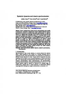
coupled map, x0 fx0 , is a solution of Eq. (1) regardless of the delays and of the connectivity of the array. Next, let us present some results of simulations that show that this state, with x0 being the nontrivial fixed point, x0 1 1=a, can be a stable solution for adequate coupling and random enough delays. The simulations were done choosing an initial configuration, xi 0 random in 0; 1, and letting the array evolve initially without coupling [in the first time interval 0 < t < max ij ]. We present results for a 4, corresponding to fully developed chaos of the individual maps, but we have found similar results for other values of a. We illustrate our findings using the small-world topology [15], but we have found similar results for random and regular (K nearest-neighbor) topologies [16], as discussed below. With both, either randomly distributed or fixed-delay times, if the coupling is large enough the array synchronizes in a spatially homogeneous state: xi t xj t 8 i; j. Figures 1 and 2 display the transition to synchronization as increases. At each value of , 100 iterates of an element of the array are plotted after transients. To do the bifurcation diagrams we varied only ; the connectivity of the array ( ij ), the delays ( ij ), and the initial configuration [xi 0] are the same for all values of . Figure 1(a) displays results for delays that are exponentially distributed, Fig. 1(b) for Gaussian distributed, Fig. 2(a) for zero delay, and Fig. 2(b) for constant delays. It can be observed that for small the four bifurcation diagrams are similar; however, for large they differ drastically: xi is constant in Figs. 1(a) and 1(b), xi x0 1 1=a, while xi varies within 0; 1 in Figs. 2(a) and 2(b). To characterize the transition to synchronization we use P the indicator 2 1=Nh i xi t hxi2 it , where h i 1

(a)

x

0.5

0.6

(b)

(e) P(τ)

i

1



PRL 94, 134102 (2005)

0.5

0.4

denotes an average over the elements of the array and h it denotes an average over time. Figures 1(c), 1(d), 2(c), and 2(d) display 2 vs for the bifurcation diagrams discussed above. It can be observed that for large there is in-phase synchronization in the four cases [xi t xj t and 2 0]; however, we note that an inspection of the time-dependent dynamics reveals that for randomly distributed delays the maps are in a steady state, while for fixed delays the maps evolve either periodically or chaotically. It can also be observed that the four plots 2 vs are similar for small [in Fig. 2(d) the array synchronizes also in a window of small ; this occurs for odd delays and was reported in [7] ]. Let us now investigate the transition from periodic or chaotic synchronization (for fixed delays) to steady-state synchronization (for random delays) by introducing a disorder parameter c that allows varying the delays from constant to distributed values. Specifically we consider the following points. (i) ij 0 Nearc, where is Gaussian distributed with zero mean and standard deviation one [17]. The delays are constant ( ij 0 ) for c 0 and are Gaussian distributed around 0 for c 0 [depending on 0 and c the distribution of delays has to be truncated to avoid negative delays; see Fig. 1(f)]. (ii) ij 0 Intc, where is exponentially distributed, positive, with unit mean. The delays are constant ( ij 0 ) for c 0 and are exponentially distributed, decaying from 0 for c 0. Figure 3(a) displays the transition between the two synchronization regimes as the randomness of the delays increases. We plot 2 vs c for different delay time distributions and 1. It can be observed that the array synchronizes for c 0 but it desynchronizes as c increases and the delays become different from each other. There is a range of values of c such that the delays are not random enough to induce steady-state synchronization; how-

0.2

(a) 0.12

0.12

0.5

1

(c)

(d) P(τ)

σ 0.04 0 0

0.5 0.5

ε

1 1

0.04 0 0

0.5

ε

5

1

10

τ

(f)

0.2

0.08

2

0.08

0

ε

i

1

ε

0

x

0.5

0 0

1

0.5

0.5

0 0

0.1

0

1

0

5

τ

0.5

FIG. 1. (a),(b) xi vs ; (c),(d) 2 vs . In (a) and (c) the delays are distributed exponentially [ 0 0, c 1:2 (see text)]; the distribution is shown in (e). In (b) and (d) the delays are Gaussian distributed [ 0 3, c 2 (see text)]; the distribution is shown in (f). The inset of (c) shows with detail the transition to synchronization: 2 decreases abruptly at 0:4, and is zero for > 0:8. N 500, a 4, and the characteristic parameter of the small-world topology is p 0:3 [15].

0.05 0 0

1 (c)

0.1

10

σ2

0 0

0 0

(b)

0.5

0.1

1 (d)

0.05 0.5 ε

1

0 0

0.5 ε

1

FIG. 2. (a),(b) xi vs ; (c),(d) 2 vs . In (a),(c) ij 0 8 i; j; in (b),(d) ij 3 8 i; j. All other parameters are as in Fig. 1.

134102-2

4

(a)

3 c

2

2

1

c

4

6

0 0

0.5

1 1.5

1

2

0 (b)

0.5

σ2 (x10−4)

σ2 (x10−4)

3

0 0

0 (a)

(b)

c

4



PRL 94, 134102 (2005)

0.2

*

0.4

c

FIG. 3 (color online). (a) 2 vs c and (b) 2 vs c . The delays are Gaussian distributed with 0 2 (䉫), 3 (4), 4 (5), 5 (䉰); exponentially distributed with 0 3 (), 4 (+), 5 (*), 6 (). 1, all other parameters are as in Fig. 1.

ever, for c large enough the array synchronizes again and 2 0. To investigate this transition we considered a normalized disorder parameter c D =h i, where h i is the average delay and D is the standard deviation of the delay distribution. By plotting 2 vs c [Figs. 3(b)] we uncover a scaling law: as h i increases the curves collapse into curves of similar shapes, and the transition to steady-state synchronization occurs for c 0:5. The value of the disorder parameter above which the arrays synchronizes in the steady state depends on the coupling strength. Figure 4(a) displays the synchronization region in the parameter space ; c. To determine the synchronization region we did simulations with different initial conditions, array connectivities, and delay time realizations: the black indicates parameters for which the array synchronized in all the simulations, while the white indicates parameters for which the array did not synchronize in any of the simulations. The gray region in the boundary of the synchronization region indicates that there are some initial conditions and/or realizations of ij and ij for which the array did not synchronize. Two different synchronization regions can be clearly distinguished: for c 0 and for c > 0:5. The former corresponds to periodic or chaotic synchronization for fixed delays, and the latter, to steady-state synchronization for distributed delays. Atay et al. [7] have recently shown that with fixed delays the synchronization depends on the array architecture: with yim t 1

1.5 0

0.6

0.5 ε

1

0

0.5 ε

1

FIG. 4. (a) Synchronization region determined numerically: black represents parameters where 2 < 107 for all the realizations of xi 0, ij , and ij . (b) Synchronization region determined from the stability analysis: black represents parameters where jmax j < 1 for all the realizations of ij and ij . The delays are Gaussian distributed with 0 3, N 100, and all other parameters are as in Fig. 1.

the same total number of links, a random network exhibits better synchronization properties than a regular network. We investigated this issue and found that with random delays the synchronization depends mainly on the average number of links per node, hbi i, and is rather independent of the architecture. Figure 5(a) displays the transition to synchronization as increases for small-world and regular arrays with distributed delays, and for comparison, Fig. 5(b) displays results for the same arrays with fixed delays. It can be observed that for distributed delays the transition to synchronization is independent of the array topology; however, it depends on the connectivity: the larger hbi i, the lower the coupling strength needed to synchronize. In contrast, for fixed delays the synchronization depends not only on the connectivity but also on the architecture: for large the arrays that have small-world topologies synchronize, but those that have regular topologies do not, in agreement with the results of [7]. Finally, let us assess the stability of the steady-state synchronized behavior found numerically by performing a statistical linear stability analysis. The delayed map Eq. (1) can be written in nondelayed form by the introduction of a set of auxiliary variables [14], yim t xi t m, where 1 i N and 0 m M with M max ij . In terms of these new NM 1 variables Eq. (1) becomes

if m 0; yi;m1 t P 1 fyi0 t N fy t if m 0; j; ij j1 ij

where ij ij =bi . Next we define a vector of NM 1 components containing information about the present and past states of the array: Y y10 ;y20 ;...; yN0 ;y11 ;y21 ;...;yN1 ;...;y1M ;y2M ;...;yNM . Equation (2) can be rewritten as Yi t 1 Fi Y1 t . . . YNM1 t and the synchronized state can be rewritten as Y x0 . . . x0 : Linearizing the equations of motion P near Y gives Yi t j fij Yj t, where the matrix F fij can be cast as a set of M 12 blocks of dimension N N [18]. We calculated the eigenvalues of F for different realizations of the connectivity and delay time distributions. The results are displayed in Fig. 4(b), where the

1

(2)

black region indicates parameters where the maximum eigenvalue of F, max , has modulus less than 1 for all ij and ij realizations, and the white region indicates parameters where max 1 for all ij and ij realizations. A very good agreement with the synchronization region determined numerically can be observed [the black region for c 0 observed in Fig. 4(a) does not appear in Fig. 4(b) because in this region the synchronized dynamics is either periodic or chaotic]. To summarize, we studied the dynamics of an ensemble of chaotic maps which interact with random delay times and found that the array synchronizes in a homogeneous

134102-3


PRL 94, 134102 (2005) (a)

(b) 0.1 σ

σ2

2

0.1 0.05 0 0

[5]

0.05 0.5 ε

1

0 0

0.5 ε

1

[6]

FIG. 5 (color online). Influence of the array architecture and connectivity. (a) Gaussian distributed delays ( 0 3, c 2) and (b) fixed delays ( ij 3 8 i; j). Small-world topology with and an average of 10 links per node (), 50 links per node (+); regular topology with 10 links per node (*); 50 links per node (4). All other parameters are as in Fig. 1.

[7] [8]

[9]

steady state. Our findings strongly resemble the so-called ‘‘amplitude (or oscillator) death’’ phenomenon, which refers to the fact that under certain conditions the amplitude of coupled oscillators shrinks to zero [19]. It has been shown that delayed coupling enhances the parameter region where oscillation death occurs [5], and that distributed delays are more stabilizing than fixed delays [13]. We think that our results are also related to the recent work of Ahlborn and Parlitz [20], who proposed a multiple delay feedback control method for stabilizing unstable steady states. Simulations of a single logistic map with several self-feedback delayed terms [i.e., Eq. (1) with j i] show that if the delay times are different, the inclusion of five or more feedback terms usually leads to chaos suppression and the stabilization of the fixed point after transients (the precise number of feedback terms needed to stabilize the fixed point depends on the delay times; these results will be reported elsewhere). Our findings provide another example of the nontrivial action of inhomogeneities and disorder, and we speculate that they might yield light on explaining the stable operation of many complex systems composed by nonlinear units which interact with each other with random communication times.

[1] A. S. Pikovsky, M. G. Rosenblum, and J. Kurths, Synchronization- A Universal Concept in Nonlinear Sciences (Cambridge University Press, Cambridge, England, 2001); Y. Kuramoto, Chemical Oscillations, Waves, and Turbulence (Springer-Verlag, Berlin, 1984); S. Bocaletti et al., Phys. Rep. 366, 1 (2002). [2] H. G. Schuster and P. Wagner, Prog. Theor. Phys. 81, 939 (1989). [3] V. K. Jirsa and M. Ding, Phys. Rev. Lett. 93, 070602 (2004). [4] E. Niebur et al., Phys. Rev. Lett. 67, 2753 (1991); U. Ernst et al., Phys. Rev. Lett. 74, 1570 (1995); S. Kim et al., Phys. Rev. Lett. 79, 2911 (1997); M. K. Stephen Yeung

[10] [11]

[12]

[13] [14] [15] [16] [17]

[18]

[19]

[20]

134102-4


and S. H. Strogatz, Phys. Rev. Lett. 82, 648 (1999); M. G. Earl and S. H. Strogatz, Phys. Rev. E 67, 036204 (2003); M. Denker et al., Phys. Rev. Lett. 92, 074103 (2004). D. V. Ramana Reddy et al., Phys. Rev. Lett. 80, 5109 (1998); D. V. Ramana Reddy et al., Phys. Rev. Lett. 85, 3381 (2000); F. M. Atay, Physica (Amsterdam) 183D, 1 (2003); R. Dodla et al., Phys. Rev. E 69, 056217 (2004). Y. Jiang, Phys. Lett. A 267, 342 (2000); C. Li et al., Physica (Amsterdam) 335A, 365 (2004). F. M. Atay et al., Phys. Rev. Lett. 92, 144101 (2004). R. Herrero et al., Phys. Rev. Lett. 84, 5312 (2000); A. Takamatsu et al., Phys. Rev. Lett. 85, 2026 (2000); A. Takamatsu et al., Phys. Rev. Lett. 87, 078102 (2001); 92, 228102 (2004); M. Dhamala et al., Phys. Rev. Lett. 92, 074104 (2004). M. Rosenblum and A. Pikovsky, Phys. Rev. Lett. 92, 114102 (2004); Phys. Rev. E 70, 041904 (2004). B. Doiron et al., Phys. Rev. Lett. 93, 048101 (2004). J. Garcı´a-Ojalvo et al., Int. J. Bifurcation Chaos Appl. Sci. Eng. 9, 2225 (1999); G. Kozyreff et al., Phys. Rev. Lett. 85, 3809 (2000); A. G. Vladimirov et al., Europhys. Lett. 61, 613 (2003). D. H. Zanette, Phys. Rev. E 62, 3167 (2000); S. O. Jeong et al., Phys. Rev. Lett. 89, 154104 (2002); T. W. Ko et al., Phys. Rev. E 69, 056106 (2004). F. M. Atay, Phys. Rev. Lett. 91, 094101 (2003). A. C. Martı´ and C. Masoller, Phys. Rev. E 67, 056219 (2003). M. E. J. Newman and D. J. Watts, Phys. Rev. E 60, 7332 (1999); Phys. Lett. A 263, 341 (1999). X. F. Wang, Int. J. Bifurcation Chaos Appl. Sci. Eng. 12, 885 (2002). Near denotes the nearest integer [Near1:7 2] while Int denotes the integer part [Int1:7 1]. We have chosen Near to have a Gaussian distribution that is symmetric with respect to 0 ; however, the results are largely independent of the precise form of the delay distribution and remain valid for ij 0 Intc. We denote the blocks as F kl , with k; l 0; . . . ; M. F kl with k > 0 have all components equal to 0, except F k1;k which are N N identity matrices. The elements of F kl with k 0 are composed by the following: (i) 1 f0 x0 , which arise from the nondelayed term in Eq. (1) and appear in the diagonal of F 00 , and (ii) =bi f0 x0 , which represent the contribution of a link and due to the random delays appear P in random positions of the blocks. There is a total of 2 i bi terms =bi f0 x0 which are distributed randomly in the blocks F 0l . More precisely, they are located at the positions i; j and j; i in the blocks F 0 ij and F 0 ji , respectively. The rest of the elements are zero. Y. Yamaguchi and H. Shimizu, Physica (Amsterdam) 11D, 212 (1984); K. Bar-Eli, Physica (Amsterdam) 14D, 242 (1985); R. E. Mirollo and S. H. Strogatz, J. Stat. Phys. 60, 245 (1990). A. Ahlborn and U. Parlitz, Phys. Rev. Lett. 93, 264101 (2004).