Random fixed point equations and inverse ... - Waterloo Fractal

Random fixed point equations and inverse problems by collage theorem H.E. Kunze1 , D. La Torre2 , E.R. Vrscay3 1

Department of Mathematics and Statistics, University of Guelph, Guelph, Ontario, Canada 2

Department of Economics, Business and Statistics, University of Milan, Italy 3

Department of Applied Mathematics, University of Waterloo, Waterloo, Ontario, Canada N2L 3G1

Abstract. In this paper we are interested in the direct and inverse problems for the following class of random fixed point equations T (w, x(w)) = x(w) where T : Ω × X → X is a given operator, Ω is a probability space and X is a complete metric space. The inverse problem is solved by recourse to the collage theorem for contractive maps. We then consider two applications: (i) random integral equations and (ii) random iterated function systems with greyscale maps (RIFSM), for which noise is added to the classical IFSM.

Keywords: Random fixed point equations, collage theorem, random integral equations, inverse problems, random iterated function systems.

1

Introduction

Let Ω denote a probability space and (X, d) a metric space. A mapping T : Ω × X → X is called a random operator if for any x ∈ X the function T (., x) is measurable. A measurable mapping x : Ω → X is called a random fixed point of a random operator T if x is a solution of the equation T (w, x(w)) = x(w).

(1)

A random operator T is called continuous (Lipschitz, contraction) if for a.e. w ∈ Ω we have that T (w, .) is continuous (Lipschitz, contraction). There are many papers in the literature that deal with such equations for single-valued and set-valued random operators (see, for example, [1,11,12,16] and the references therein). Solutions of random fixed point equations and inclusions are usually produced by means of stochastic generalizations of classical fixed point theory. The main purpose of this paper is to provide solutions to both the forward and inverse problems of random fixed point equations of the form in Eq. (1).

H.E. Kunze1 , D. La Torre2 , E.R. Vrscay3

2

in the case that the random maps T are contractive. Solutions to inverse problems are accomplished by using appropriate random collage theorems, which are stochastic analogs of their classical counterparts. We then present two applications of our method: (i) random integral equations and (ii) random iterated function systems with greyscale mappings.

2

Fixed point equations and collage theorem

In this section, we recall some basic facts regarding contraction maps that will be used in later sections. Let (X, d) denote a complete metric space. Then T : X → X is contractive if there exists a c ∈ [0, 1) such that d(T x, T y) ≤ cd(x, y) for all x, y ∈ X.

(2)

We normally refer to the infimum of all c values satisfying Eq. (2) as the contraction factor of T . Theorem 1. (Banach) Let (X, d) be a complete metric space. Also let T : X → X be a contraction mapping with contraction factor c ∈ [0, 1). Then there exists a unique x ¯ ∈ X such that x ¯ = Tx ¯. Moreover, for any x ∈ X, d(T n x, x ¯) → 0 as n → ∞. Theorem 2. (Continuity theorem for fixed points [6]) Let (X, dX ) be a complete metric space and T1 , T2 be two contractive mappings with contraction factors c1 and c2 and fixed points y¯1 and y¯2 , respectively. Then dX (¯ y1 , y¯2 ) ≤

1 dX,sup (T1 , T2 ) 1 − min{c1 , c2 }

(3)

where dX,sup (T1 , T2 ) = sup d(T1 (x), T2 (x)).

(4)

x∈X

Of course, Banach’s fixed point theorem provides a mechanism to solve the forward problem of the fixed point equation x = T x: Given a contraction T , construct, or at least approximate, its fixed point x ¯. And the continuity theorem establishes that small changes in a contraction mapping produce small changes in the associated fixed points. We may state a formal mathematical inverse problem associated with the fixed point equation x = T x as follows: Given a target element y and an  > 0, find a contraction map T () (perhaps from a suitable family of operators) with fixed point x ¯() such that d(y, x ¯()) < . If one is able to solve such an inverse problem to arbitrary precision, i.e.,  → 0, then one may identify the target y as the fixed point of a contractive operator T on X. In practical applications, however, it is not generally possible to find such solutions to arbitrary accuracy nor is it even possible to search for such contraction maps. Instead, one makes use of the following result, which is a simple consequence of Banach’s fixed point theorem.

Random fixed point equations

3

Theorem 3. (“Collage theorem” [4]) Let (X, d) be a complete metric space and T : X → X a contraction mapping with contraction factor c ∈ [0, 1). Then for any y ∈ X, 1 d(y, x ¯) ≤ d(y, T y), (5) 1−c where x ¯ is the fixed point of T . Note that the approximation error d(y, x ¯) is bounded above by the so-called collage distance d(y, T y). Most practical methods of solving such inverse problems, for example, fractal image coding [7,15], search for an operator T for which the collage distance is as small as possible. In other words, they seek an operator T that maps the target y as close as possible to itself. This inverse problem procedure, often referred to as collage coding, is most often performed by considering a parametrized family of contraction maps Tλ , λ ∈ Λ ⊂ Rn , and then minimizing the collage distance d(y, Tλ y). Finally, we mention another interesting result which is a simple consequence of Banach’s fixed point theorem. Theorem 4. (“Anti-collage theorem” [18]) Let (X, d) be a complete metric space and T : X → X a contraction mapping with contraction factor c ∈ [0, 1). Then for any y ∈ X, 1 d(y, T y), (6) d(y, x ¯) ≥ 1+c where x ¯ is the fixed point of T .

3

Random fixed point equation: parametric approach

Let (Ω, F, µ) be a probability space and let (X, dX ) be a complete metric space. (X, d) is said to be a Polish space if it is a separable complete metric space. Let T : Ω × X → X be a given operator. We look for the solution of the equation T (ω, x(ω)) = x(ω)

(7)

for a.e. ω ∈ Ω\A and µ(A) = 0. Suppose that the operator T satisfies the inequality d(T (ω, x), T (ω, y)) ≤ c(ω)d(x, y), (8) where c(ω) : Ω → X satisfies c(ω) ≤ c < 1 a.e., with ω ∈ Ω\A and µ(A) = 0. When T satisfies this property, we say that T is a c(ω)-contraction. Then for ω ∈ Ω\A there exists a unique point x(ω) ∈ X. It is clear that the uniqueness makes sense when one doesn’t consider sets of measure zero. Once again, the inverse problem can be formulated as: Given a function x : Ω → X and a family of operators Tλ : Ω × X → X find λ such that x is the solution of random fixed point equation Tλ (ω, x(ω)) = x(ω). (9) As simple consequences of the collage and continuity results of the preceding sections, we have the following results.

H.E. Kunze1 , D. La Torre2 , E.R. Vrscay3

4

Corollary 1. (“Regularity conditions”) Let (Ω, F, µ) be a probability space and let (X, dX ) be a complete metric space. Let T : Ω × X → X be a given c(ω)contraction. Then dX (x(ω1 ), x(ω2 )) ≤

1 sup d(T (ω1 , x), T (ω2 , x)) 1 − c x∈X

(10)

Corollary 2. (“Continuity Theorem”) Let (Ω, F, µ) be a probability space and let (X, dX ) be a complete metric space. Let Ti : Ω × X → X be two given ci (ω)-contractions, i = 1, 2. Then 1 sup d(T1 (ω, x), T2 (ω, x)) 1 − min{c1 , c2 } x∈X

dX (x1 (ω), x2 (ω)) ≤

(11)

Theorem 5. (“Collage Theorem”) Let (Ω, F, µ) be a probability space and let (X, dX ) be a complete metric space. Let T : Ω × X → X be a given c(ω)contraction. Then 1 1 dX (x(ω), T (ω, x(ω))) ≤ dX (x(ω), x ¯(ω)) ≤ dX (x(ω), T (ω, x(ω))), 1+c 1−c (12) a.e. ω ∈ Ω, where x ¯(ω) is the solution of T (ω, x ¯(ω)) = x ¯(ω).

4

Random fixed point equations: global approach

Consider now the space Y of all measurable functions x : Ω → X. If we define the operator T˜ : Y → Y as (T˜y)(ω) = T (ω, x(ω)) the solutions of this fixed point equation on Y are the solutions of the random fixed point equation T (ω, x(ω)) = x(ω). Suppose that the metric dX is bounded, that is dX (x1 , x2 ) ≤ K for all x1 , x2 ∈ X. So the function ψ(ω) = dX (x1 (ω), x2 (ω)) : Ω → R is an element of L1 (Ω) for all x1 , x2 ∈ Ω. We can then define on the space Y the following function Z dY (x1 , x2 ) = dX (x1 (ω), x2 (ω))dω. (13) Ω

Theorem 6. The space (Y, dY ) is a complete metric space. Proof. It is trivial to prove that dY is a metric when we consider that x1 = x2 if x1 (ω) = x2 (ω) a.e. ω ∈ Ω. To prove the completeness we follow the trail of the proof of Theorem 1.2 in [13]. Let xn be a Cauchy sequence in Y . So for all  > 0 there exists n0 such that for all n, m ≥ n0 we have dY (xn , xm ) < . Let  = 3−k so you can choose an increasing sequence nk such that dY (xn , xnk ) < 3−k for all n ≥ nk . So choosing n = nk+1 we have dY (xnk+1 , xnk ) < 3−k . Let  Ak = ω ∈ Ω : dX (xnk+1 (ω), xnk (ω)) > 2−k . (14) Then µ(Ak )2−k ≤

Z Ak

dX (xnk+1 (ω), xnk (ω))dw ≤ 3−k ,

(15)

Random fixed point equations

and so µ(Ak ) ≤

5


2 k . 3

T∞ S Let A = m=1 k≥m Ak . We observe that   [ X µ Ak  ≤ µ(Ak ) k≥m

k≥m


2 m X  2 k 3
, = ≤ 3 1 − 23 k≥m and so

 m 2 µ(A) ≤ 3 3

(16)

(17)

for all m, and this implies µ(A) = 0. Now for all ω 6∈ Ω\A there exists m0 (ω) such that for all m ≥ m0 we have ω 6∈ Am and so dX (xnm+1 (w), xnm (ω)) < 2−m . This implies that xnm (ω) is Cauchy for all ω 6∈ Ω\A and so xnm (ω) → x(ω) using the completeness of X. This also implies that x : Ω → Y is measurable, that is, x ∈ Y . To prove xn → x in Y we have that Z dY (xnk , x) = dX (xnk (w), x(ω))dω ZΩ = lim dX (xnk (ω), xni (ω))dω Ω i→+∞ Z dX (xnk (ω), xni (ω))dω ≤ lim inf i→+∞

Ω

= lim inf dY (xnk , xni ) ≤ 3−k i→+∞

(18)

for all k. So limk→+∞ dY (xnk , x) = 0. Now we have dY (xn , x) ≤ dY (xn , xnk ) + dY (xnk , x) → 0

(19)

when k → +∞. We have the following theorem. Theorem 7. Suppose that (i) for all x ∈ Y the function ξ(ω) := T (ω, x(ω)) belongs to Y , (ii) dY (T˜x1 , T˜x2 ) ≤ cdY (x1 , x2 ) with c < 1. Then there exists a unique solution of T˜x ¯=x ¯, that is, T (w, x ¯(ω)) = x ¯(ω) for a.e. ω ∈ Ω. We observe that the hypothesis (i) can be avoided if X is a Polish space. In fact the following result holds. Theorem 8. [11] Let X be a Polish space, that is, a separable complete metric space, and T : Ω × X → X be a mapping such that for each ω ∈ Ω the function T (ω, .) is c(ω)-Lipschitz and for each x ∈ X the function T (., x) is measurable. Let x : Ω → X be a measurable mapping; then the mapping ξ : Ω → X defined by ξ(ω) = T (ω, x(ω)) is measurable.

H.E. Kunze1 , D. La Torre2 , E.R. Vrscay3

6

Corollary 3. Let T : Ω × X → X be a mapping such that for each ω ∈ Ω the function T (ω, .) is a c(ω)-contraction. Suppose that for each x ∈ X the function T (., x) is measurable. Then there exists a unique solution of the equation T˜x ¯=x ¯ that is T (ω, x ¯(ω)) = x ¯(ω) for a.e. ω ∈ Ω. The inverse problem can be formulated as: Given a function x ¯ : Ω → X and a family of operators T˜λ : Y → Y find λ such that x ¯ is the solution of random fixed point equation T˜λ x ¯=x ¯, (20) that is, Tλ (ω, x ¯(ω)) = x ¯(ω).

(21)

As a consequence of the collage and continuity theorems, we have the following. Corollary 4. Suppose that (i) for all x ∈ Y the function ξ(ω) := T (ω, x(ω)) belongs to Y , (ii) dY (T˜x1 , T˜x2 ) ≤ cdY (x1 , x2 ) with c < 1. Then for any x ∈ Y , 1 1 dY (x, T˜x) ≤ dY (x, x ¯) ≤ dY (x, T˜x), 1+c 1−c

(22)

where x ¯ is the fixed point of T˜, that is, x ¯(ω) := T (ω, x ¯(ω)).

5

Random integral equations

Consider now the space X = {x ∈ C([0, 1]) : kxk∞ ≤ M } endowed with the usual d∞ metric and let (Ω, F, p) be a given probability space. Let φ : R × R → R be such that |φ(t, z1 ) − φ(t, z2 )| ≤ K|z1 − z2 |, where 0 ≤ K < 1. Then the following results hold. Theorem 9. Let Z T (ω, x) =

t

φ(s, x(s))ds + x0 (ω). 0

If Z

1

|φ(s, 0)|ds + |x0 (ω)| ≤ M (1 − K)

(23)

0

then T : Ω × X → X. Proof. It is trivial to prove that T (ω, x) is a continuous function. To show that it belongs to X, we have, for a fixed ω ∈ Ω, Z 1 kT (ω, ·)k∞ ≤ |φ(s, x(s))|ds + |x0 (ω)| Z0 1 Z 1 ≤ |φ(s, x(s)) − φ(s, 0)|ds + |φ(s, 0)|ds + |x0 (ω)| 0

0

Random fixed point equations

Z 1 ≤ Kkxk∞ + |φ(s, 0)|ds + |x0 (ω)| Z 1 0 ≤ KM + |φ(s, 0)|ds + |x0 (ω)|,

7

(24)

0

and the theorem is proved. Consider now the operator T˜ : Y → Y where Y = {x : Ω → X, x is measurable} and

t

Z

[(T˜x)(ω)](t) =

(25)

φ(s, [x(ω)](s))ds + x0 (ω)

(26)

0

for a.e. ω ∈ Ω. We have used the notation [x(ω)] to emphasize that for a.e. ω ∈ Ω [x(ω)] is an element of X. We have the following result. Theorem 10. T˜ is a contraction on Y . Proof. Computing, we have Z dY (T˜x, T˜y) = d∞ (T (ω, x(ω)), T (ω, y(ω)))dω ZΩ ≤ kT (ω, x(ω)) − T (ω, y(ω))k∞ dω Ω Z t Z ≤ sup |φ(s, [x(ω)](s)) − φ(s, [y(ω)](s))|dsdω Ω t∈[0,1]

Z

0 t

Z

≤

K|[x(ω)](s) − [y(ω)](s)|dsdω

sup Ω t∈[0,1]

0

Z ≤K

d∞ (x(ω), y(ω))dω = KdY (x, y).

(27)

Ω

By Banach’s theorem we have the existence and uniqueness of the solution of the equation T˜x = x. For a.e. (ω, s) ∈ Ω × [0, 1] we have Z s φ(t, x(ω, t))dt + x0 (ω). (28) x(ω, s) = 0

5.1

Inverse problem

In what follows, we consider the following form for the kernel of T : φ(t, z) = a0 + a1 t + a2 z.

(29)

Once again, suppose that u is the target function and x0 (ω) is a random variable with unknown mean µ. The goal is to find the values a0 , a1 , a2 and µ that satisfy, as best as possible, the random fixed point equation Z s x(ω, s) = (a0 + a1 t + a2 x(ω, t)) dt + x0 (ω). (30) 0

H.E. Kunze1 , D. La Torre2 , E.R. Vrscay3

8

These values will be determined by collage coding, as discussed in [14]. If the function ω → x(ω, s) is integrable for each s ∈ [0, 1] we can take the expectation value E(x(ω, s)) = x(s) on both sides to give Z s x(s) = (a0 + a1 t + a2 x(t)) dt + µ. (31) 0

Now assume that we have a sample of observations x(ω1 , s), x(ω2 , s), . . . , x(ωn , s) of the variable x(ω, s) from which the mean is constructed: n

x∗n (s)

1X x(ωi , s). = n i=1

(32)

Using the sample mean x∗n we approximate the problem in (30) as follows: Z s x∗n (s) = (a0 + a1 t + a2 x∗n (t)) dt + µ. (33) 0

Example: For each i, we construct an approximation of u(ωi , x) by iterating the map related to (30), where we have set a0 = 1, a1 = 2, and a2 = 0.75. (We could solve the equivalent initial value problem, but wish to have the slight imprecision of such an approximation rather than an exact solution.) We generate 30 observations and use collage coding to treat the inverse problem outlined above for x∗30 (s). See Figure 1 for an illustration of the situation. Collage coding yields

Fig. 1. Graphs of the 30 observed solutions (thin curves) and y = x∗30 (s) (thick curve) in the cases (left to right): µ = 0.8, σ 2 = 0.3; µ = 1.5, σ 2 = 0.5; µ = 3.0, σ 2 = 1.0.

the values of a0 , a1 , a2 and µ given in Table 1. Note that the values of a0 , a1 , and a2 are correct to five decimal places. The minimal collage values of µ are very good. One might replace the observations x(ωi , s) by measurements at a set of points sj , j = 1, . . . , M , and then fit a polynomial to the data points, using this function as the approximation of the observation. Or one might discretize the collage distance at mesh points induced by the observation points. In both cases, good results are obtained.

Random fixed point equations True Values

9

Minimal Collage Parameters

µ

σ2

0.8

0.3

1.00000 2.00000 0.75000 0.78515

1.5

0.5

1.00000 2.00000 0.75000 1.47525

3.0

1.0

1.00000 2.00000 0.75000 2.95050

a0

a1

a2

µ

Table 1. Collage coding results for the random Picard operator (values to five decimal places).

6

Random IFSM

The method of iterated function systems with greyscale maps (IFSM), as formulated by Forte and Vrscay (see [8]), can be used to approximate a given element u of L2 ([0, 1]). We consider the case in which u : [0, 1] → [0, 1] and the space  X = u : [0, 1] → [0, 1], u ∈ L2 . (34) The ingredients of an N -map IFSM on X are [8,9] 1. a set of N contractive mappings w = {w1 , w2 , . . . , wN }, wi (x) : [0, 1] → [0, 1], most often affine in form: 0 ≤ si < 1,

wi (x) = si x + ai ,

i = 1, 2, . . . , N,

(35)

2. a set of associated functions—the greyscale maps—φ = {φ1 , φ2 , . . . , φN }, φi : R → R. Once again, affine maps are usually employed: φi (t) = αi t + βi ,

(36)

αi , βi ∈ [0, 1]

(37)

with the conditions and 0≤

N X

(αi + βi ) ≤ δ < 1.

(38)

i=1

Here δ > 0 is a given fixed parameter which will be needed for reasons to be described below. Associated with the N -map IFSM (w, φ) is the fractal transform operator T ∗ , the action of which on a function u ∈ X is given by (T ∗ u)(x) =

N X

0

φk (u(wk−1 (x))),

(39)

k=1

where the prime means that the sum operates on all those terms for which wk−1 is defined.

H.E. Kunze1 , D. La Torre2 , E.R. Vrscay3

10

Theorem 11. [8] T ∗ : X → X and for any u, v ∈ X we have d2 (T ∗ u, T ∗ v) ≤ Cd2 (u, v) where C=

N X

(40)

1

si2 αi .

(41)

i=1

In the case that C < 1, then T ∗ is contractive on X, implying the existence of a unique fixed point u ¯ ∈ X such that u ¯ = T ∗u ¯. We now formulate a Random IFSM fractal transform that corresponds to the deterministic fractal transform in Eq. (39). Let (Ω, F, p) be a probability space and consider now the following operator T : X × Ω → X defined by T (u, ω) = T ∗ (u) + x0 (ω),

(42)

where x0 is a random variable with mean µ and |x0 (ω)| < 1 − δ for all ω ∈ Ω. Let Y = {u : Ω → X, u is measurable} (43) and consider the function ψ(ω) := dX (u1 (ω), u2 (ω)) = ku1 (ω) − u2 (ω)k2 .

(44)

From the hypotheses it is clear that ψ(ω) ∈ L1 (Ω). We know that (Y, dY ) is a complete metric space where Z dY (u1 , u2 ) = ku1 (ω) − u2 (ω)k2 dω. (45) Ω

Obviously the function ξ(ω) := T (ω, u(ω)) = T ∗ u(ω) + x0 (ω) belongs to Y because T ∗ is Lipschitz on X and u is measurable. If we define T˜ : Y → Y where T˜u = ξ we have Z ˜ ˜ dY (T u1 , T u2 ) = kT ∗ u1 (ω) + x0 (ω) − T ∗ u2 (ω) − x0 (ω)k2 dω ΩZ ≤C ku1 (ω) − u2 (ω)k2 dω Ω

= CdY (u1 , u2 ).

(46)

So there exists u ¯ ∈ Y such that T˜u ¯ = u ¯, that is, u ¯(ω) = T (ω, u ¯(ω)) for a.e. ω ∈ Ω. 6.1

Inverse problem for RIFSM and “denoising”

In the previous section we proved that there exists a unique element u ¯:Ω→X which is measurable and satisfies u ¯(ω) = T ∗ u ¯(ω) + x0 (ω) for a.e. ω ∈ Ω and u ¯(ω, x) = (T ∗ u ¯(ω))(x) + x0 (ω) =

N X k=1

0

φk (¯ u(ω, wk−1 (x))) + x0 (ω)

(47)

Random fixed point equations

11

for a.e. x ∈ [0, 1]. Now suppose that the function u ¯(ω, x) : Ω × [0, 1] → R is integrable and let Z Z u ¯(x) = [¯ u(ω)](x)dω = u ¯(ω, x)dω. (48) Ω

Ω

Thus Eq. (47) becomes u ¯(x) =

N X

0

φk (¯ u(wk−1 (x))) + µ.

(49)

k=1

That is, the expectation value of u ¯(ω, x) is the solution of a deterministic N -map IFSM on X (cf. Eq. (39)) with a shift µ. (Such functions that are added to an IFSM—in this case the constant function g(x) = µ—are known as condensation functions.) Now suppose that we have N observations, u(ω1 ), u(ω2 ), . . ., u(ωn ), of the variable u(ω), from which we construct the mean n

u∗n (x) =

n

1X 1X [u(ωi )](x) = u(ωi , x). n i=1 n i=1

(50)

Given u∗n ∈ X, we now outline a method to approximate solutions of the inverse problem in Eq. (49) using the N -map IFSM of the previous section. First, we employ a fixed set of N contraction maps wi (x) = si x + ai , as defined in Eq. (35). Associated with these maps, we then determine the optimal greyscale maps φi (t) defined in Eq. (36), that is, the greyscale maps that provide the best approximation u∗n (x) ≈ (T ∗ u∗n )(x) =

N X

0

φk (u∗n (wk−1 (x))) + µ.

(51)

k=1

Using the Collage Theorem, this amounts to finding the αi and βi parameters that minimize the squared collage distance, ∆2 = ku∗n − T ∗ u∗n k22 ≤

Z X N I k=1

0

kφk (u∗n (wk−1 (x))) + µ − u∗n (x)k2 dx,

(52)

where I = [0, 1]. In many practical treatments, it is convenient to use maps wi (x) that satisfy the following conditions: SN SN (i) k=1 wk (I) = I, i.e., the sets Ik “tile” I, and k=1 Ik = (ii) m(wi (I) ∩ wj (I)) = 0 for i 6= j, where m denotes Lebesgue measure. IFS maps wi satisfying the latter condition are said to be nonoverlapping over I. In this case the constraints in Eq. (38) reduce to 0 ≤ αi + βi ≤ δ < 1 for all i.

12

H.E. Kunze1 , D. La Torre2 , E.R. Vrscay3

Example: We define the following nonoverlapping N -map IFS over [0, 1]:   1 i−1 wi , i = 1, . . . , N wi (x) = x + N N with grey level maps φi (t) = αi t + βi , i = 1, . . . , N . In this example, we set N = 20 and consider the target function u(x) = 0.4(x − 1)2 + 0.1.

(53)

The problem is now to determine the optimal greyscale map parameters, αi and βi , that satisfy the constraints αi + βi < 0.5,

1 ≤ i ≤ N.

(54)

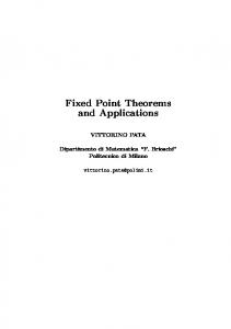
These constraints are enforced to ensure that the RIFSM operator T (u, ω) = T ∗ (u) + x0 (ω) maps X × Ω to X, where the x0 values are selected from a scaled normal distribution with mean 0.3. Using iterations of T , we produce a collection of 25 different RIFSM observations. In Figure 2 are presented the graphs of these different realizations, along with the graphs of our target function and the mean of the realizations. It now remains to minimize the squared L2 collage distance Eq. (52) for the mean of our realizations, subject to the constraints in Eq. (54). The solution of this quadratic programming problem yields optimal greyscale parameters αi and βi as well as the mean µ of additive noise distribution. In this particular simulation, the result is µ = 0.31229. Other simulations with different noising but with the same mean µ = 0.3 and variance σ 2 = 0.1 also yield quite good results. For thirty different runs, the minimal collage value of µ produced by the mean of 25 realizations always lies in the interval [0.22, 0.38]. If we increase the number of observations, the accuracy improves. For example, with 100 observations, we find that the minimal collage µ = 0.3117. Good results are obtained for other noise parameters. As expected, if the amplitude of the noise is decreased, the results improve dramatically. Remark: The random IFSM operator T defined in Eq. (42) and used in the above example may be viewed as a deterministic IFSM with additive noise. The mean function u∗n (x) constructed from the n observations may be viewed as a kind of denoising of these noisy signals, except that it contains the unknown mean value µ. The solution of the inverse problem in Eq. (51) produces an approximation of µ which can then be subtracted from u∗n (x) to yield the denoised signal. 6.2

Formal solution of the inverse problem

Finally, we outline how the inverse problem associated with RIFSM can, in principle, be solved to arbitrary accuracy, using a procedure defined in [8]. We

Random fixed point equations

13

Fig. 2. The thin curves are 25 different realizations of solutions to our RIFSM. The lower thick curve is our target function u(x) = 0.4(x − 1)2 + 0.1. The thick curve in the middle is the mean of the realizations.

return to the squared collage distance function associated with an N -map IFSM as defined in Eq. (52), which may be written as a quadratic form: ∆2 = z T Az + bT z + c,

(55)

where z = (α1 , . . . αk , β1 , . . . , βk , µ). The maps wk are chosen from an infinite set W of fixed affine contraction maps on [0, 1] which satisfy the following properties. Definition 1. We say that W generates an m-dense and nonoverlapping family A of subsets of I if for every  > 0 and every B ⊂ I there exists a finite set of integers ik , ik ≥ 1, 1 ≤ k ≤ N , such that (i) A = ∪N k=1 wik (I) ⊂ B, (ii) m(B\A) < , and (iii) m(wik (I) ∩ wil (I)) = 0 if k 6= l, where m denotes Lebesgue measure. Let W N = {w1 , . . . wN }

(56)

14

H.E. Kunze1 , D. La Torre2 , E.R. Vrscay3

be the N truncations of w. Let ΦN = {φ1 , . . . , φN } be the N vector of affine grey level maps. Let z N be the solution of the previous quadratic optimization problem and ∆2N,min = ∆2N (z N ). In [8], the following result was proved Theorem 12. ∆2N,min → 0 as N → ∞. From the Collage Theorem, the inverse problem may be solved to arbitrary accuracy.

Acknowledgements This work has been written during a research visit by DLT to the Department of Applied Mathematics of the University of Waterloo. DLT thanks ERV for this opportunity. For DLT this work has been supported by COFIN Research Project 2004. This work has also been supported in part by research grants (HEK and ERV) from the Natural Sciences and Engineering Research Council of Canada (NSERC), which are hereby gratefully acknowledged.

References 1. R.P. Agarwal, D. O’Regan, Fixed point theory for generalized contractions on spaces with two metrics, J. Math. Anal. App. 248, 402-414, 2000. 2. M.F. Barnsley, Fractals Everywhere, Academic Press, New York, 1989. 3. M.F. Barnsley and S. Demko, Iterated function systems and the global construction of fractals, Proc. Roy. Soc. London Ser. A, 399, 243-275, 1985. 4. M.F. Barnsley, V. Ervin, D. Hardin and J. Lancaster, Solution of an inverse problem for fractals and other sets, Proc. Nat. Acad. Sci. USA, 83, 1975-1977, 1985. 5. T.D. Benavides, G. Lopez Acedo, H-K. Xu, Random fixed points of set-valued operators 124, 3, 1996. 6. P. Centore and E.R. Vrscay, Continuity of fixed points for attractors and invariant meaures for iterated function systems, Canadian Math. Bull. 37, 315-329, 1994. 7. Y. Fisher, Fractal Image Compression, Theory and Application, Springer Verlag, NY, 1995. 8. B. Forte and E.R. Vrscay, Solving the inverse problem for function and image approximation using iterated function systems, Dynamics of Continuous, Discrete and Impulsive Systems, 1, 2, 1995. 9. B. Forte and E.R. Vrscay, Theory of generalized fractal transforms, Fractal Image Encoding and Analysis, NATO ASI Series F, Vol 159, ed. Y.Fisher, Springer Verlag, New York, 1998. 10. B. Forte and E.R. Vrscay, Inverse problem methods for generalized fractal transforms, in Fractal Image Encoding and Analysis, ibid. 11. S. Itoh, Random fixed point theorems with an application to random differential equations in banach spaces, J. Math. Anal. App. 67, 261-273, 1979. 12. S. Itoh, A random fixed point theorem for a multivalued contraction mapping, Pacific. J. Math. 68, 1, 85-90, 1977.

Random fixed point equations

15

13. M. Kisielewicz, Differential inclusions and optimal control, Mathematics and its applications, Kluwer, 1991. 14. H. Kunze and E.R. Vrscay, Solving inverse problems for ordinary differential equations using the Picard contraction mapping, Inverse Problems 15, 745-770, 1999. 15. N. Lu, Fractal imaging, Academic Press, NY, 2003. 16. D. O’Regan, N. Shahzad, R.P. Agarwal, Random fixed point theory in spaces with two metric, J. App. Math. Stoch. Anal. 16, 2, 171-176, 2003. 17. D. O’Regan, A fixed point theorem for condensing operators and applications to Hammerstein integral equations in Banach spaces, Computers Math. Applic. 30, 9, 39-49, 1995. 18. E.R. Vrscay and D. Saupe, Can one break the ‘collage barrier’ in fractal image coding?, in Fractals: Theory and Applications in Engineering, ed. M. Dekking, J. Levy-Vehel, E. Lutton and C. Tricot, Springer Verlag, London, 307-323, 1999.