Random model for RNA interference yields scale free network

Random model for RNA interference yields scale free network Duygu Balcan1 and Ay¸se Erzan1,2 1

arXiv:q-bio/0310027v1 [q-bio.GN] 21 Oct 2003

2

Department of Physics, Faculty of Sciences and Letters Istanbul Technical University, Maslak 34469, Istanbul, Turkey G¨ ursey Institute, P.O.B. 6, C ¸ engelk¨ oy, 34680 Istanbul, Turkey (Dated: June 5, 2018)

We introduce a random bit-string model of post-transcriptional genetic regulation based on sequence matching. The model spontaneously yields a scale free network with power law scaling with γ = −1 and also exhibits log-periodic behaviour. The in-degree distribution is much narrower, and exhibits a pronounced peak followed by a Gaussian distribution. The network is of the smallest world type, with the average minimum path length independent of the size of the network, as long as the network consists of one giant cluster. The percolation threshold depends on the system size. Keywords: self-organisation, gene regulation networks, RNA interference, bitstring models, evolution I.

INTRODUCTION

Although biology on the whole is a “knowledge based” discipline, with a strong traditional bias towards a reverse engineering approach to evolution, and a “form follows function” approach, prominant workers in the field have stressed that natural selection could very well have operated on complex structures already present in the prebiotic world. Eigen [1] pointed out that non-linear out of equilibrium systems were capable of amplifying random fluctuations participating in feed-back loops, while Kauffman [2, 3] introduced random Boolean networks as null models of the genetic regulatory mechanism, and showed that they could spontaneously give rise to a great degree of complexity. Meanwhile, within the last two decades, we have learned a great deal about Self-Organized Criticality [4], namely the spontaneous emergence of scale free structures in open systems far from equilibrium, driven by conserved fluxes. Thus, within a statistical mechanics context, it is much more natural to consider an ensemble of different states among which complex structures arise spontaneously. Evolutionary processes can be regarded as inducing dynamics on the distribution of states in this high dimensional phase space. In this paper we introduce a null model for gene interactions resulting in the regulation of gene expression. This model is based on sequence matching on a random bit-string representation of the chromosome and is therefore radically different from the random Boolean networks which have been considered before [2, 3, 5, 6, 7, 8]. It can be considered as an out of equilibrium system subject to a constant mutation rate, achieving a steady state invariant under further mutations. We present simulation results which display many qualitative features of gene regulation networks found in nature [9, 10]. We find that the in- and out- degree distributions are qualitatively different from each other, the out-degree distribution exhibiting power law decay with γ n(kout ) ∼ kout , with γ = −1 and log- periodic oscillations for relatively small k. The in-degree distribution, on the other hand, is much more localized. The network has smallest world characteristics, with

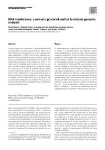
FIG. 1: The random sequence of symbols representing a chromosome. The “2” represents a start or stop sign for a gene, and the 0’s and 1’s code the genes. The arrows indicate that one gene sequence is embedded in another one.

the cluster diameter, or the average minimum path length being essentially independent of the cluster size as long as the network consists of one cluster. The average clustering coefficients for the in and out bonds have been calculated as 0.648 and 0.034 respectively. It is interesting to note that the clustering coefficients for the in-bonds behave much like for classical random networks [11], while the out-bonds have a clustering coefficient typical of scale free networks. [12, 13] In section 2, we will first motivate and then define the model. In section 3, we will present our simulation results. In section 4, we consider a toy model which mimics some of the features we observe in our simulations, and indicate ways in which this toy model may be improved in order to provide insights into how our basic model works. Section 5 contains our conclusions and a discussion. II.

MODELLING RNA INTERFERENCE A.

Genomic regulatory networks

Protein networks, which are an important component of transcriptional gene regulation networks [14, 15], display a scale free structure, with the out-degree distribution characterised by a power law n(k) ∼ k γ , with the exponent γ ≃ −2.5. [9, 10] Gene regulation networks actually operate at many different levels. [16] Posttranscriptional gene regulation, or RNA interference [17], is a mechanism where RNA strips may go and directly

2 bind upon complementary segments on messenger RNA destined to be translated into some protein, thereby suppressing the production of this protein. Although we are not aware of a scaling analysis of post-transriptional gene interaction, it would be a fair guess to assume that interaction complexes of various sizes may arise in this type of interaction as well. In all protein-protein or intra-genomic interactions, as well as the transcription and translation mechanism itself, essential lock-and key mechanisms are in operation. For normal translation to take place, rRNA in the ribosomes must be able to recognize and match the different amino acids and the corresponding three-letter anticodon on the mRNA. In this, the rRNA is aided by the intermediary tRNA, which assumes a very specific three dimensional structure depending on the amino acid to which it binds. In transcriptional gene regulation, certain proteins known as transcription factors (TF) must first be synthesized, and then go and bind onto specific “promoter” sites preceding the coding part of a gene, in order that the RNA polymerase might start transcribing the DNA code into the mRNA. Conversely, the binding of other proteins onto the same promoter sites may block the binding of the TF, and thereby block the production of the mRNA. [17, 18] In both cases, such binding presupposes steric and chemical specificity. In RNA interference, the short interfering RNA (siRNA) strips bind onto complementary sequences on the mRNA, via Watson-Crick base pairing. [17, 19] Although it seems, from the above, as if there is a great diversity in these lock-and-key mechanisms, it should be realised that they all eventually match linear codes, even though this matching may take a few intermediary steps. The three dimensional structures (so called secondary structures) which come into play either in tRNA or the TF, are actually determined by either the sequence of ribo-nucleic acids on the tRNA, or the sequence of amino acids (primary structure) of the protein constituting the TF. Clearly the simplest is direct Watson-Crick base pairing between complementary sequences, and it is this latter, as it appears in RNA interference, which we will take to be the paradigm for our model. In fact we will further simplify the matching condition to consist of the identity relation rather than complementarity, since both are one-to-one, we believe that this should not change our results. B.

The Model

The model is defined as follows. We postulate a “chromosome” to consist of a sequence of fixed length L, of independently and identically distributed random numbers with the probability distribution P (x) = pδ(x − 2) + (1 − p)/2[δ(x − 1) + δ(x)]

(1)

We define a “gene” to consist of a sequence of 0’s and 1’s situated between the ith and i + 1st occurance of the

FIG. 2: Different kinds of vertices allowed on our directed random network. While the in or out-neighbors of a vertex may or may not be connected to each other, in the case of the third configuration, with a pair of mixed bonds, the neighboring nodes are necessarily connected as shown, due to transitivity.

symbol “2,” and we will denote the ith gene by Gi = {xi,1 , xi,2 , . . . xi,ℓi } i = 1, . . . , s

(2)

where xi,µ 6= 2, µ = 1, . . . ℓi and ℓi is the length of the ith gene. We have used periodic boundary conditions, but one could just as well agree to end the chromosome always with a “2” at the L + 1st site. Then s X

ℓi = L − s ,

(3)

i

where s is the number of genes (the number of times the symbol 2 appears) on the chromosome. Let nℓ be the number of genes of length ℓ. It obeys the sum rule L−s X

nℓ = s .

(4)

ℓ=0

For a given number s of genes, the number of possible realisations of a given set {nℓ } is s! K[{nℓ }] = QL−s ℓ=0

nℓ !

,

(5)

and the most probable distribution n(ℓ) can easily be found by using Lagrange multipliers, to be n(ℓ) = Lp2 (1 − p)ℓ , in the limit of large L. With these definitions we obtain a sequence of genes, seperated from each other by the symbol 2. (See Fig. (1)). In case there are more than one consecutive 2’s, they will be considered to bracket null genes. Clearly, for large L, the number of non-null genes, N , will fluctuate around N = Lp − Lp2 . Each of the non-null genes constitutes a node in our gene regulation network. The interactions do not depend on the proximity of the genes along the chromosome. We define the adjacency matrix wij by the matching condition such that n wij = 1 Gi ⊂ Gj . (6) 0 otherwise By Gi ⊂ Gj we mean xi,µ = xj,µ+ν for µ = 1, . . . ℓi for at least one integer ν such that 0 ≤ ν ≤ ℓj − ℓi . Note that wij = 1 implies that ℓi ≤ ℓj ; in the case of the

3

p=0.1, L=5000 4

n(kout)

3

2

1

0 100

300

400

FIG. 3: The out degree distribution, for p = 0.1 and L = 5000.

p=0.05, L=15 000 4.0 3.5 3.0 2.5 2.0 1.5 1.0 0.5 0.0 100

Pij = P (ℓi , ℓj ) ,

200

kout

n(kout)

equality, wij = 1 if and only if the two sequences Gi and Gj are identical, i.e., congruent. Thus, two genes are said to interact if the sequence Gi occurs at least once as an unbroken subsequence of Gj , i.e., if one can be embedded in the other at least once. Clearly this adjacency (or connectivity) matrix is directed. Moreover connectivity is “transitive” in the sense that wij = wjk = 1 implies that wik = 1. The latter condition gives rise to a preferential attachment of incoming bonds to large genes, while small genes have an enhanced distribution of out-bonds. However, we will see in the next section that the degree distribution is scale free for the out-bounds, but not for the in-bonds. A simple argument tells us that our network is of the smallest world [12] type. If we take the out-bonds, we see that due to the transitivity, any two successive edges linking say vertex ij and jk, necessarily imply the exis(o) tence of another directed edge ik. Thus lmin ≡ 1, as long as the network consists of a single cluster. The in-bonds (i) follow the same argument, giving lmin ≡ 1 for a network with one giant cluster. The question of whether a giant cluster always exists or whether we can identify the analog of a “percolation threshold” we will address in the next section, where we will also report numerical results for the minimum path length for undirected bonds (i.e., ignoring the directionality of the edges.) We expect that the qualitative behaviour of the network should not depend on p as long as p is bounded away from the percolation threshold. Requiring the number of vertices, N , to be larger than unity, i.e., N = Lp − Lp2 = Lp(1 − p) > 1 gives p(1 − p) > 1/L (however this lower limit turns out not to be tight enough, i.e., pc > 1/L). The average gene size, again in the limit of large L is hℓi = (1 − p)/p. The obvious requirement for a non-trivial network, that hℓi > 1 yields p < 1/2. We therefore expect to find scaling behaviour, if any, for pc < p < 1/2. The elements wij of the connectivity matrix are equal to unity with probabilities

200

(7)

300

400

500

600

700

800

kout

which depend on the lengths (ℓi , ℓj ) through ℓi and ν = ℓj − ℓi . It is trivial to see that  ℓ 1 P (ℓ, ℓ) = 2

FIG. 4: The out degree distribution for p = 0.05 and L = 15000.

.

(8)

We may make a mean field theory type of approximation to P (ℓ, ℓ + ν) by neglecting the correlations between overlapping subsequences of Gj , and obtain, P (ℓ, ℓ + ν) ≃

 ℓ 1 (1 + ν) . 2

(9)

In the Appendix we have computed P (ℓ, ℓ + ν) explicitly for ν = 1, 2. However, so far it has not been possible to extract the form of the degree distribution analytically.

The directed graph gives rise to different kinds of vertices, shown in Fig.(2), which allow different classes of clustering coefficients C. Let kout (i), kin (i), k(i), be, respectively, the out- degree, in-degree and the total degree of the vertex i. The clustering coefficient at a given vertex i is defined as Ci =

2E(i) k(i)[k(i) − 1]

(10)

where E(i) is the number of edges connecting the nearest

4 neighbors of i. Thus it is the number of pairs of nearest neighbors directly connected to each other, normalized by the largest number of such connections possible. We may extend this concept to directed graphs and define, 2Eout (i) kout (i)[kout (i) − 1]

2.5

(11) 2.0

and similiarly for Cin , where Eout (i) (respectively Ein (i)) are the number of edges connecting out (in) nearest neighbors of i. Note that any pair of incoming and outgoing bonds passing through i necessarily defines a triangle, due to transitivity, as shown in Fig.( 2). Thus, the clustering coefficient may be conveniently decomposed as Ci =

kin (i) kout (i) + Ein (i) + Eout (i) . k(i)[k(i) − 1]/2

(12)

This is a null model in the sense that no assumptions have been made as to the fitness of any particular type of interaction; the resulting interactions depend only on the random sequences coded in the genes and on the distribution of gene lengths. This random network provides the “tabula rasa” on which we assume natural selection will subsequently act. As such, it is of great interest to determine the properties of the null network, which turn out to be highly non-trivial. This is the task to which we turn in the next section. III.

SIMULATION RESULTS

To characterize the network defined by our model, we generated random chromosomes as defined above. The statistical properties of the network obtained from the totally random chromosome were checked to be invariant under a constant mutational load, with a mutation probability of 0.01. A mutation is affected as follows. If the symbol (x) occupying the site to be mutated happens to be a 0 or 1, then it is flipped, i.e., we set x = mod2 (x+1). If x = 2, then it exchanges places with either its right or left nearest neighbor, with equal probability. It should be noted that the first case corresponds to a substitutional mutation, whereas the second to a shifting of the position of the start sign which shifts the reading frame of the gene. The latter gives rise to far-reaching modifications, since the three-letter codes corresponding to the different amino acids will be completely modified along the whole gene if the reading frame is shifted. The most remarkable property of the random network generated in this way is that it has a scale free out-degree distribution, and a qualitatively different in-degree distribution which is much less broad, with a pronounced narrow peak followed by a Gaussian peak. These qualitative behaviours match the results found on protein and genomic networks to a surprising extent. [9, 10] We display in Figs.(3,4) the out-degree distribution n(kout ) for two sets of parameters, namely L = 5000, p = 0.1 and for L = 15000 p = 0.05, with, the number of

ln[ n(kout) ]

Cout (i) =

p=0.1, L=5000 3.0

1.5 1.0 0.5 0.0 -0.5

0

1

2

3

4

5

6

ln[ kout ]

FIG. 5: The log-log fit to the envelope of the out-degree distribution shown in Fig.(3). The slopes of the dashed and continuous lines are -0.9 and -0.39, respectively.

genes fluctuating around N = 450 and N = 712, respectively. The data have been averaged over 500 independent realizations. The distributions, which are strongly γ′ , log periodic, with a power law envelope nm (kout ) ∼ kout have the same characteristic behaviour for the two cases. The fits to the envelope of the peaks are shown in Figs.(5,6). We see a marked break in the log-log fit for larger p, with a crossover from γ ′ ≃ −1 to γ ′ = −0.45 ± 0.06 at about ln(kout ) = 2.5. This crossover behavior is just off-scale in Fig.( 6), as can be seen in Fig.( 7), with the incipient scaling with a power of −1 again extending out to ln(kout ) ≃ 2. It is also worthwhile mentioning that the integral over the peaks to the rightmost of the out-degree distribution simply gives the network size N , as it should, because these peaks come from the smallest genes of unit length which are embedded in all the other genes. Introducing a larger lower cutoff to the gene size (i.e., a cutoff bigger than unity) would somewhat restrict the range of kout , but also yield cleaner scaling behaviour for large values of kout by effectively eliminating these peaks. It should be noticed that for kout ≤ 100, the dips in the degree distribution are about evenly spaced on the logarithmic scale, with a scale factor of 1/2. We conjecture that each individual peak corresponds to a particular gene-length ℓ. (This conjecture is borne out by comparing the integrals under the peaks with nℓ for p = 0.1, L = 5000 but is much more noisy for p = 0.05, L = 15000). Increasing ℓ by unity, exactly halves the leading contribution to the to kout , from genes of length ℓ. To get a better grip on the degree distribution, we nu-

5

p=0.05, L=15 000

p=0.05, L=15 000 1.0

25

ln[ n (k out) ]

3.3

0.8 20

0.6

n(kout)

ln[ n(kout) ]

0.4 0.2 0.0

3.0 2.7 2.4 2.1

15 1.8 1.5

10

0.0

-0.2

0.5

1.0

1.5

2.0

ln[ k out ]

-0.4

5

-0.6 -0.8

0 1

2.5

3.0

3.5

4.0

4.5

5.0

5.5

6.0

2

3

6.5

4

5

6

7

kout

ln[ kout ]

FIG. 6: The log-log fit to the envelope of the out-degree distribution for p = 0.05, L = 15000 (Fig.(4)). The fit is to a slope of -0.46.

FIG. 7: The initial peak of the out-degree distribution for p = 0.05 and L = 15000, and the double logarithmic graph of the same, showing incipient power law behaviour with the power −0.89.

merically integrated the curves in Figs.(3,4). The result is shown for p = 0.05 in Fig.(8). We find that

p=0.05, L=15 000 750

Z

kout

n(z)dz ∼ ln(kout ) ,

(13)

γ+1 where numerically γ + 1 < or a very small power, ∼ kout 0.1, at least for kout that are not too large. Thus we are led to believe that the overall out degree distribution scales like γ n(kout ) ∼ kout f (kout /N ) ,

(14)

with γ = −1.0 ± 0.1. The scaling function f (x) ∼ const. for x ≪ 1, and is log-periodic for intermediate values of its argument. Scaling breaks down for x ∼ O(1). Note that γ is smaller in absolute value than that reported for real gene regulation networks [9, 10, 15], thus evolution seems to have narrowed the distribution somewhat, restricting the number of genes that may be affected by any one gene. The in-degree distribution, which we display in Fig.(9) shows two peaks. The second can be fit to a Gaussian, as shown in Fig.(10). The first peak is more skewed than a Poissonian, but may be fitted reasonably well by a distribution of the form f (x) ∼ (x − x0 )δ exp[−ξ(x − x0 )], where δ = 2.2 and ξ = 0.15. (Fig.(11)). The total degree distribution again displays a modulated structure, as can be seen in Fig.(12). We have already discussed that the network will behave trivially either for very small N (all very large genes with very small probabilities for interaction) or for large p (i.e., p > 1/2) where most of the chromosome will be

700 650 600

N (k out)

N (kout ) ≡

550 500 450 400 0

100

200

300

400

500

600

700

800

kout

FIG. 8: The wavy line is the cumulative out degree distribution for p = 0.05, L = 15000. The dashed line is a logarithmic 0.11 fit, while the continuous one ∼ kout .

occupied by non-coding partitions (the symbol 2), and many null genes. We have determined the threshold value, pc , below which the the genes are too few and too long, such that the single giant cluster breaks up into more than one component. The results are reported in Table I, for L ranging from 15000 to 1000, and undirected edges. Although we have only a few points, the

6

p=0.1, L=5000

5

p=0.1, L=5000 5

4

4

3

n(kin)

n(kin)

3

2

2

1

1 0 0

50

100

150

200

250

300

0

kin

10

20

30

40

50

kin FIG. 9: The in-degree distribution for p = 0.1 and L = 5000. The in-degree distribution is much narrower that the outdegree distribution and displays two peaks.

FIG. 11: The first peak of the in-degree distribution, with the tail of the Guassian distribution subtracted. The fits are to a Poisson distribution (continuous line) exp(−z)z k /k! with z = k computed from the data points, and the function f (k) = 0.09(k − 10)2.2 exp[−0.15(x − 10)] (dashed line).

p=0.1, L=5000 1.2

p=0.05, L=15 000

1.0 0.8

6

0.6

5

0.4

4

n(k)

ln[ n(k in) ]

7

0.2

3 2

0.0 0

500

1000

1500

(kin-(kin)0)

2000

1

2 0 0

100

200

300

400

500

600

700

800

k FIG. 10: The second peak of the in-degree distribution for p = 0.1 and L = 5000 can be fit to a Gaussian. FIG. 12: The total degree distribution for p = 0.05, L = 15000.

dependence (see Fig. 13) fits a power law, with pc ∼ L−α , with α ≃ 3/4, within the range explored. In the limit of L → ∞, pc → 0, but less fast than 1/L. On the other hand our expectations that there is a reasonably large interval of p’s (pc < p < 1/2) where the results do not depend quantitatively on the precise value of p are borne out, as can be seen from our calculations for the minimum average path length for undirected edges.

We argued in section II that as long as there is a single giant cluster, the directed minimum path length is identically 1. For undirected paths this is no longer true and we must determine hlmin i numerically. Nevertheless, we can show that lmin ≤ 4. Note that for p > pc , there will be an abundance of short genes of unit length, which will

7 Table II

Table I

L 15000 5000 1500 1000

hN i 177 112 83 54

pc 0.012 0.023 0.059 0.086

TABLE I: The “percolation threshold” for strings of different length L. The average number of non-null genes at the percolation threshold is also reported.

L 15000 10000 5000 2500 2000 1750 1650

hN i 717 479 239 120 95 83 79

hlmin i 1.669 1.670 1.670 1.670 1.669 1.672 1.673

TABLE II: The average minimum path length for undirected edges, with p = 0.05, for different L. Table III

-2.5

ln[ pc ]

-3.0

p 0.013 0.014 0.016 0.018 0.02 0.05 0.1 0.48

-3.5

-4.0

-4.5

6.5

7.0

7.5

8.0

8.5

9.0

9.5

L 15000 15000 15000 15000 15000 15000 10000 1500

hN i 194 209 237 267 295 717 452 374

hlmin i 1.858 1.851 1.84 1.82 1.81 1.669 1.543 1.360

10.0

ln[ L ]

TABLE III: The average minimum path length hlmin i for undirected edges, for different p and L. Note that hlmin i varies very little over the entire range from p ≃ pc to p ≃ 1/2.

FIG. 13: Dependence of the “percolation threshold” on L. The power law fit gives pc ∼ L−3/4 .

contain the symbol 0 or 1 with equal probability. These will have outgoing edges to all the typical genes which have an admixture of 0s and 1s, so that most such genes will be certainly linked by paths of length at most equal to 2. The “worst case” is that of atypical cases of all 1’s all or all 0’s which require at least one intermediate typical gene to link up (11111 − 1 − 011100 − 0 − 00000), which gives max(lmin ) = 4. We have calculated hlmin i for fixed p and different L. If we consider undirected edges and find that it at most depends very weakly on N , the number of vertices. We find, e.g., for L ranging from 1650 to 15000, and p = 0.05 that hlmin i ranges only from 1.673 to 1.699. (Table II) Fixing the length L and varying p (Table III) shows again that as long as hlmin i is defined, i.e., just above the “percolation threshold” it is already very close to the value it will have for larger p. The clustering coefficients are markedly different for the in- and out-degree distributions, as well as the total connectivity. We find, for p = 0.05 and L = 15000, < Cout >= 0.034, < Cin >= 0.648 and < C >= 0.534.

We have verified in the last case that this clustering coefficient is reproduced by computing the average total degree per node and deviding by the total number of nodes, i.e., < C >≃< k > /N . Thus, the total connectivity behaves very much like in classical random graphs.

IV.

ANALYTICAL RESULTS ON TOY MODEL

In this section we would like to present a number of the results which may be obtained from a hierarchical model. In particular, we would like to exploit the transitivity property, to compute certain properties of a toy version of our original model. Let us consider a tree network, with a branching ratio b. Take all connections emanating from nodes at the mth generation to the ones at the m + 1st generation, to be directed. If one applies the transitivity rule, then this automatically generates further connections that link directly a node at the mth generation to all the nodes below it on the same branch of the tree. Then, the out degree (we will drop the index “out” from now on) of a

8 node at the mth level will be k(m) =

M−m−1 X m′ =0

′

bm =

bM−m − 1 , b−1

(15)

where M is the total number of levels and k(m) ∼ bM−m for large M − m, which we may safely assume. The frequency of the nodes at the mth level is bm . This gives, for the out-degree distribution,   1 . (16) n(k) ∼ const. k We now introduce redundancies within the same level. Let a fraction r of the b downstream neighbors emanating from any node be identical to each other, with r = am , b−1 < a < 1 being some constant. The nodes that are identical within any given level are connected to each other by two-way bonds within the sub-branch where they are located. I will call this subset of nodes the clones at any given level. This means that the out-degree k of any one of these nodes is now k ′ = (am b)bM−m , since each interconnected node inherits all the downstream neighbors of the am b clones to which it is connected. The interconnections between nodes further downstream do not introduce any further change in k ′ (m), since all the nodes that they can connect are already connected to the nodes at level m. The number of clone-nodes (not all identical to each other, but only in groups of am b) is clearly am bm . Then, the out-degree distribution of the nodes belonging to the clone-sets becomes,  ′ γ k n(k ′ ) = bγ−1 (17) N where N = bM and with γ=

ln a + ln b . ln a − ln b

(18)

Note that under our assumptions above, −1 < γ < 0. For large enough k this then becomes the leading contribution to the out degree distribution, rather than γ = −1. V.

CONCLUSIONS AND DISCUSSION

The model we have presented for the scaling behaviour of gene interaction, more specifically RNA interference, turns out to be a rich model which is worthwhile to investigate in its own right, as well as providing a highly structured starting point on which further evolutionary pressures could act. We have checked that the statistical properties of the network are robust under random point mutations. Thus, the scale free random network may be seen as the attrator for a process starting from, say, a sequence of uniform

genes, subjected to random point mutations over a very long time period. The scale free steady state can be considered as the outcome of a process of self-organization under random perturbations. In conclusion it is worthwhile to note that in RNA interference, longer RNA chains are cut up by the “Dicer” enzyme into smaller segments, siRNA [17], which can be conveniently matched with complementary sequences in a larger number of mRNAs. This trick would change the power of the out-degree distribution from that found here. Acknowledgements One of us (AE) would like to gratefully acknowledge partial support from the Turkish Academy of Sciences. It is a pleasure to thank B. Bollobas and J.-P. Eckmann for useful conversations. APPENDIX We would like to compute the probabilities P (ℓ, ℓ′ ) in Eq.(7). For successive ν = ℓ′ − ℓ > 0, it is convenient to define subsequences of Gj of length (λ) ℓi with a shift λ, 0 ≤ λ ≤ ν, such that gij ≡ {xj,1+λ , xj,2+λ , . . . xj,ℓi +λ }. Then, we can obtain P (ℓ, ℓ′ ) (0) in terms of joint probabilities like P(Gi 6= gij , Gi = (1)

gij ), etc. Thus, (0)

= P(Gi = gij )

P (ℓ, ℓ)

(0)

(0)

P (ℓ, ℓ + 1) ...

(1)

= P(Gi = gij ) + P(Gi 6= gij , Gi = gij ) (0)

= P(Gi = gij ) + . . .

P (ℓ, ℓ + ν)

(0)

(1)

6 gij , . . . , Gi = Gλij ) + P(Gi 6= gij , Gi = + ... (ν) (1) (0) 6 gij , . . . , Gi = gij ) + P(Gi = 6 gij , Gi = (0)

(1)

Let us display P(Gi 6= gij , Gi = gij ) for greater clarity. We have (0)

(1)

P(Gi = 6 gij , Gi = gij ) = ! ℓi ℓ µ−1 Y X
Y h δxi,m xj,m 1 − δxi,µ ,xj,µ δxi,n xj,n+1 i µ=1 m=1   = 2−ℓi 1 − 2−ℓi .

n=1

In particular we find

  P (ℓ, ℓ + 1) = 2−ℓ 1 + 1 − 2−ℓ   = 2−ℓ 2 − 2−ℓ P (ℓ, ℓ + 2) = 2−ℓ 3 − 2−ℓ+1 −


1 1 − 2−2ℓ 3

Note that the probabilities P do not depend upon the particular gene, except through the lengths of the sequences, as the genes do not overlap, and each of the symbols are independently and identically distributed, with equal probability, over 0 and 1.

9

[1] M. Eigen, Naturwissenschaften 10, 58 (1971) [2] S.A. Kauffman, J. Theor. Biol. 22, 437 (1969). [3] S. Kauffmann, The Origins of Order: Self-organization and Selection in Evolution (Oxford University Press, N.Y. 1993) [4] P. Bak, C. Tang and K. Wiesenfeld, Phys. Rev. Lett. 59, 381 (1987); Phys. Rev. A 38, 364 (1988); K. Sneppen, P. Bak, H. Flyvberg, M.H. Jensen, Proc. Natl. Acad. Sci. 92, 5209 (1995). [5] H. Atlan, F. Fogelman-Soulie, J. Salomon, et al., Random Boolean Networks Cybernet. Syst. 12,103 (1981) [6] B. Derrida, G. Weisbuch, J. Phys. (Paris) 47, 1297-1303 (1986) [7] B.Derrida and Y. Pomeau, Europhys. Lett. 1, 45 (1986). [8] B. Derrida, H.Flyvberg, J. Phys. A 20 L1107 (1987). [9] S. Maslov and K. Sneppen, Science 296, 910 (2002). [10] S.Maslov, Midterm Conference COSIN on “Growing Networks and Graphs in Statistical Physics, Finance, Biology and Social Systems”, Rome, 1-5 September 2003 (see

this issue). [11] P. Erd¨ os and . R´enyi, Publ. Math. Inst. Hung. Acad. Sci. 5, 17 (1960). [12] S.N. Dorogovstsev and J.F.F. Mendes, Adv. Phys. 51, 1079 (2002). [13] R. Albert and A.-L. Barabasi, Rev. Mod. Phys. 74, 47 (2002). [14] N.A. Campbell, J.B. Reece, Biology (Addison Wesley, San Francisco, 2002), p. 363-368. [15] R. V. Sole and R. Pastor-Satorras, “Complex Networks in Genomics and Proteomics,” S. Bornholdt and H.G.Schuster eds., Handbook of Graphs and Networks (Wiley-VCH Verlag, Berlin 2002). [16] T. Maniatis and R. Reed, Nature 416, 499 (2002). [17] G.J. Hannon, Nature 418, 244 (2002). [18] B. Alberts et al., Molecular Biology of the Cell (Garland Science, N.y., 2002) p. 375 ff. [19] Op. cit., p. 451-52.