7 Dec 2018 - ... positioning each vertex at a uniformly chosen location in the hyperbolic space, and then. 1. arXiv:1812.03002v1 [physics.soc-ph] 7 Dec 2018 ...
Scale-free network clustering in hyperbolic and other random graphs
arXiv:1812.03002v1 [physics.soc-ph] 7 Dec 2018
Clara Stegehuis, Remco van der Hofstad, and Johan S.H. van Leeuwaarden Department of Mathematics and Computer Science Eindhoven University of Technology December 10, 2018 Abstract Random graphs with power-law degrees can model scale-free networks as sparse topologies with strong degree heterogeneity. Mathematical analysis of such random graphs proved successful in explaining scale-free network properties such as resilience, navigability and small distances. We introduce a variational principle to explain how vertices tend to cluster in triangles as a function of their degrees. We apply the variational principle to the hyperbolic model that quickly gains popularity as a model for scale-free networks with latent geometries and clustering. We show that clustering in the hyperbolic model is non-vanishing and self-averaging, so that a single random graph sample is a good representation in the largenetwork limit. We also demonstrate the variational principle for some classical random graphs including the preferential attachment model and the configuration model.
1
Introduction
Scale-free networks feature in many branches of science, describing connectivity patterns between particles through large graphs with strong vertex-degree heterogeneity, often modeled as a power law that lets the proportion of vertices with k neighbors scale as k −τ . Statistical analysis suggests that the power-law exponent τ in real-world networks often lies between 2 and 3 [3, 27, 40, 55], so that the vertex degree has a finite first and infinite second moment. With such power laws, vertices of extremely high degrees (also called hubs) are likely to be present, and cause scalefree properties such as small distances [34, 48], fast information spreading [25, 50, 12] and the absence of percolation thresholds [39, 50]. Power-law degrees and hubs also crucially influence local properties such as the abundance of certain subgraphs like triangles and cliques [49, 54, 35]. For several decades now, scientists are building the theoretical foundation for scale-free networks, using a large variety of mathematical models and approaches. Classical models like the preferential attachment model and the hidden-variable model generate mathematically tractable random graphs with power-law degrees, and were successful in explaining some of the key empirical observations for distances and information spreading. The average distance in the scale-free random graph models, for instance, was shown to scale as log log n in the network size n [23, 34, 26, 20], in agreement with the small distances measured in real-world networks. Another empirically observed scale-free property is the tendency of vertices to cluster together in groups with relatively many edges between the group members [31]. The preferential attachment model and the hidden-variable model, however, both have vanishing clustering levels when the network size grows to infinity, rendering these models unfit for modeling group formation in the large-network limit. We therefore employ the hyperbolic model, which in recent years has emerged as a new scale-free network model [43, 4, 13, 30, 15]. The model creates a random graph by positioning each vertex at a uniformly chosen location in the hyperbolic space, and then 1
c(k)
c(k)
c(k)
100 10−1
10−1
10−1
10−2
10−2 101
102
(a)
103
k
10−2
−3
10
101
102
103
(b)
104
k
101
102
103
104
k
(c)
Figure 1: c(k) for (a) the WordNet information network [46], (b) the TREC-WT10g web graph [5] and (c) the Catster/Dogster social network [44]. connecting pairs of vertices as a function of their locations. The hyperbolic model is mathematically tractable and capable of matching simultaneously the three key characteristics of real-world networks: sparseness, power-law degrees and clustering. The degree of clustering can be measured in terms of the local clustering coefficient c(k), the probability that two neighbors of a degree-k vertex are neighbors themselves, and also in terms of the average clustering coefficient C that gives an overall indication of the clustering in the network. Ample empirical evidence shows that the function c(k) generally decreases in k according to some power law [55, 45, 54, 11, 21, 42], which suggest that the network can be viewed as a collection of subgraphs with dense connections within themselves and sparser ones between them [51]. Randomizing real-world networks while preserving the shape of the c(k)-curve produces networks with very similar component sizes as well as similar hierarchical structures as the original network [22]. The shape of c(k) also influences the behavior of networks under percolation [52, 47]. Figure 1 shows the c(k)-curves for three different networks: an information network describing the relationships between English words (Fig. 1a), a technological network describing web pages and their hyperlinks (Fig. 1b) and a social network (Fig. 1c). While these three networks are very different, their c(k)-curves share several similarities. First of all, c(k) decays in k in all three networks. Furthermore, for small values of k, c(k) is high in all three networks, indicating the presence of non-trivial clustering. Taking the hyperbolic model as the network model, we obtain a precise characterization of clustering in the hyperbolic model by describing how the clustering curve k 7→ c(k) scales with k and n. We also obtain the scaling behavior for C from the results for c(k). Studying the local clustering coefficient c(k) is equivalent to studying the number of triangles where at least one of the vertices has degree k. We develop a novel conceptual framework, a variational principle, that finds the dominant such triangle in terms of the degrees of the other two vertices. This variational principle exploits the trade-off present in power-law networks: highdegree vertices are well connected and therefore participate in many triangles, but high-degree vertices are rare because of the power-law degree distribution. Lower-degree vertices typically participate in fewer triangles, but occur more frequently. The variational principle finds the degrees that optimize this trade-off and reveals the structure of the three-point correlations between triplets of vertices that dictate the degree of clustering. In Section 2 we present the variational principle and apply it to the hyperbolic model to find the typical relation between clustering, node degree and the power-law exponent of the degree distribution. In Section 3 we present an extended version of the variational principle that can deal with general subgraphs and apply it to characterize the sample-to-sample fluctuations of clustering in the hyperbolic model. As it turns out, the clustering curve k 7→ c(k) and the global clustering coefficient C in the hyperbolic model are non-vanishing and self-averaging as n → ∞. We then proceed to apply the variational principle to the hidden-variable model, the preferential attachment model and the random intersection graph in Section 4.
2
Figure 2: A hyperbolic random graph on 500 vertices with degree exponent τ = 2.5. Vertices are embedded based on their radial and angular coordinates.
2
Hyperbolic model
We now discuss the hyperbolic model in more detail, introduce the generic variational principle to characterize clustering, and then apply the variational principle to the hyperbolic model. The hyperbolic random graph samples n vertices in a disk of radius R = 2 log(n/ν), where the density of the radial coordinate r of a vertex p = (r, φ) is ρ(r) = β
sinh(βr) cosh(βR) − 1
(1)
with β = (τ − 1)/2. Here ν is a parameter that influences the average degree of the generated networks. The angle φ of p is sampled uniformly from [0, 2π]. Then, two vertices are connected if their hyperbolic distance is at most R. The hyperbolic distance of points u = (ru , φu ) and v = (rv , φv ) satisfies cosh(d(u, v)) = cosh(ru ) cosh(rv ) − sinh(ru ) sinh(rv ) cos(∆θ).
(2)
Two neighbors of a vertex are likely to be close to one another due to the geometric nature of the hyperbolic random graph. Therefore, the hyperbolic random graph contains many triangles [32]. Furthermore, the model generates scale-free networks with degree exponent τ [43] and small diameter [28]. Figure 2 shows that vertices with small radial coordinates are often hubs, whereas vertices with larger radial coordinates usually have small degrees, which we explain in more detail in the Methods section. We use this relation between radial coordinate and degree to find the most likely triangle in the hyperbolic model in terms of degrees as well as radial coordinates.
2.1
Variational principle
The variational principle deals with the probability of creating a triangle between a vertex of degree k and two other uniformly chosen vertices, which can be written as X P (4k ) = P (4 on degrees k, d1 , d2 ) P (d1 , d2 ) , (3) (d1 ,d2 )
where the sum is over all possible pairs of degrees (d1 , d2 ), and P (d1 , d2 ) denotes the probability that two uniformly chosen vertices have degrees d1 and d2 . We then let the degrees d1 and d2 scale as nα1 and nα2 and find which degrees give the largest contribution to (3). Due to the power-law degree distribution, the probability that a vertex has degree proportional to nα scales as n−(τ −1)α . The maximal summand of (3) can then be written as max P (4 on degrees k, nα1 , nα2 ) n2+(α1 +α2 )(1−τ ) .
α1 ,α2
3
(4)
If the optimizer over α1 and α2 is unique, and attained by α1∗ and α2∗ , then we can write the probability that a triangle is present between a vertex of degree k and two randomly chosen vertices as � � ∗ ∗ ∗ ∗ P (4k ) ∝ P 4 on degrees k, nα1 , nα2 n(α1 +α2 )(1−τ ) . (5) The local clustering coefficient c(k) is defined as �the expected number of triangles containing a uniformly chosen vertex of degree k divided by k2 . Therefore, � � ∗ ∗ ∗ ∗ c(k) ∝ n2 k −2 P 4 on degrees k, nα1 , nα2 n(α1 +α2 )(1−τ ) . (6) Thus, if we know the probability that a triangle is present between vertices of degrees k, nα1 and nα2 for some random graph model, the variational principle is able to find the scaling of c(k) in k and the graph size n. Let us now explain why the variational principle (6) applies to a fairly large class of random graphs. Suppose a model assigns to each vertex some parameters that determine the connection probabilities (radial and angular coordinates in case of the hyperbolic random graph). The variational principle can then be applied as long as the vertex degree can be expressed as some function of the vertex parameters, so that the probability of triangle formation between three vertices can be viewed as a function of the vertex degrees, and one can search for the optimal contribution to (4).
2.2
Local clustering
To compute c(k) for the hyperbolic model, we calculate the probability that a triangle is present between vertices of degrees k, nα1 and nα2 using the variational principle. Vertices with small radial coordinates are often hubs, whereas vertices with larger radial coordinates usually have small degrees. We will use this relation between radial coordinate and degree to find the most likely triangle in the hyperbolic model in terms of degrees as well as radial coordinates. For a point i with radial coordinate ri , we define its type ti as ti = e(R−ri )/2 .
(7)
Then, if Di denotes the degree of vertex i, by [53] ti = Θ(Di ).
(8)
Furthermore, the ti ’s follow a power-law with exponent τ [10], so that the degrees have a power-law distribution as well. The ti ’s can be interpreted as the weights in a hidden-variable model [10]. Because the degrees and the types of vertices have the same scaling, we investigate the probability that two neighbors of a vertex of type k connect. We compute the probability that a triangle is formed between a vertex of degree k, a vertex i with ti ∝ nα1 and a vertex j with tj ∝ nα2 with α1 ≤ α2 . We can write this probability as P (4 on types k, nα1 , nα2 ) = P (k ↔ nα1 ) P (k ↔ nα2 ) P (nα1 and nα2 neighbors connect) .
(9)
The probability that two vertices with types ti and tj connect satisfies by [10] P (i ↔ j | ti , tj ) ∝ min (2νti tj /(πn), 1) .
(10)
Therefore, the probability that a vertex of type k connects with a randomly chosen vertex of type nα1 can be approximated by P (k ↔ nα1 ) ∝ min(knα1 −1 , 1). (11) We now compute the order of magnitude of the third term in (9), which is more involved than the first two terms. Two neighbors of a vertex are likely to be close to one another, which increases
4
√ (a) τ < 5/2: For k � n the two other vertices have degree proportional to n/k, whereas √ for k � n the other two vertices have degree proportional to k.
(b) τ > 5/2: The other two vertices have constant degree across the entire range of k.
Figure 3: Typical triangles containing a vertex of degree k (dark red) in hyperbolic random graphs. A vertex of degree nα has radial coordinate close to R − α, so that the optimal triangle degrees can be translated back to their radial coordinates in the disk. the probability that they connect. Two vertices with types ti and tj and angular coordinates φi and φj connect if the relative angle between φi and φj , ∆θ, satisfies [10] ∆θ ≤ Θ (2νti tj /n) .
(12)
W.l.o.g., let the angular coordinate of the vertex with degree k be 0. For i and j to be connected to a vertex with φ = 0, by (12) φi and φj must satisfy − Θ(min(knα1 −1 , 1)) ≤ φi ≤ Θ(min(knα1 −1 , 1)),
− Θ(min(knα2 −1 , 1)) ≤ φj ≤ Θ(min(knα2 −1 , 1)).
(13)
Because the angular coordinates in the hyperbolic random graph are uniformly distributed, φi and φj are uniformly distributed in these ranges. By (12), vertices i and j are connected if their relative angle is at most 2νnα1 +α2 −1 . (14) Thus, the probability that i and j connect is the probability that two randomly chosen points in the intervals (13) differ in their angles by at most (14). Assume that α2 ≥ α1 . Then, the probability that i and j are connected is proportional to � � nα1 +α2 −1 α1 α2 P (n and n neighbor connect) ∝ min ,1 min(knα2 −1 , 1) = min(nα1 max(nα2 −1 , k −1 ), 1).
(15)
Thus, (4) reduces to max n(α1 +α2 )(1−τ ) min(knα1 −1 , 1) min(knα2 −1 , 1) min(nα1 max(nα2 −1 , k −1 ), 1).
α1 ,α2
(16)
Because of the min(knα2 −1 , 1) term, it is never optimal to let the max term be attained by nα2 −1 . Thus, the equation reduces further to max n(α1 +α2 )(1−τ ) min(knα1 −1 , 1) min(knα2 −1 , 1) min(nα1 k −1 , 1).
α1 ,α2
5
(17)
c(k) 100
c(k) 100 10−1
10−1
c(k) 10−1
τ =2.2 τ =2.5 τ =2.8
10−2 10−3
−2
10
101
102
10−3
10−4
τ = 2.2 τ = 2.5 τ = 2.8
10−4
10−5
103
104
k
10−6 0 10
(a) Hyperbolic random graph with ν = 1.
τ =2.25 τ =2.50 τ =2.75
10−2
101
102
103
104
105
(b) Hidden-variable model
10−5 0 10
k
101
102
103
104
105
k
(c) Preferential attachment model with m = 4
Figure 4: Simulations of c(k) for three different models with n = 106 . The solid lines correspond to averages over 104 network realizations and the dashed lines indicate the asymptotic slopes of (19), (36) and (45). The maximizers over α1 ≤ α2 are given by 0 0 τ > 25 , (n , n ), √ (nα1 , nα2 ) ∝ (k, k) τ < 52 , k � n, √ (n/k, n/k) τ < 52 , k � n.
(18)
Combining this with (6) shows that −1 k c(k) ∝ k 4−2τ 2τ −6 5−2τ k n
τ > 52 , √ τ < 52 , k � n, √ τ < 52 , k � n.
(19)
This result is more detailed than the result in [43], where the scaling c(k) ∼ k −1 was predicted for fixed k. We find that this scaling only holds for the larger values of τ , while for τ < 5/2 the decay of the curve is significantly different, which was simultaneously found in [37]. Note that for τ > 5/2, the c(k) curve does not depend on n. For τ < 5/2 the dependence on n is only present for large values of k. Interestingly, the exponent τ = 5/2 is also the point where the maximal contribution to a bidirectional shortest path in the hyperbolic random graph changes from highdegree to lower-degree vertices [7]. Also, the optimal triangle structures contain higher vertex degrees for τ < 2.5 than for τ > 2.5 (see Fig. 3). Figure 4a confirms the asymptotic slopes (19) with extensive simulations.
3
Self-averaging behavior 2
We say that c(k) is self-averaging when Var (c(k)) /E [c(k)] → 0 as n → ∞, so that the sample-tosample fluctuations of c(k) vanish in the large-network limit. When c(k) fails to be self-averaging, the fluctuations persist even in the large-network limit, so that the average of c(k) over many network realizations cannot be viewed as a reliable descriptor of local clustering. We will now show how to apply the variational principle (6) to constrained subgraphs larger than triangles, 2 which leads to a complete characterization of Var (c(k)) /E [c(k)] in the large-network limit. The variational principle can hence determine for any value of k whether c(k) is self-averaging or not. In this way we are able to show that for the hyperbolic random graph, c(k) is self-averaging for all values of τ ∈ (2, 3) and all k. This implies that for large enough n, one sample of the hyperbolic random graph is sufficient to obtain the characteristic behavior of c(k).
6
3.1
Extended variational principle
To show that c(k) is self-averaging, we first study E [c(k)]. In the variational principle (4), we obtained the typical number of triangles where one vertex has degree k by putting the hard constraint α1 , α2 ≤ 1/(τ − 1) on the degrees of the other two vertices in the triangle. If we relax this constraint, we can compute E [c(k)]. This quantity can be interpreted as the value of c(k) obtained after simulating many hyperbolic random graphs, and taking the average value of c(k) over all these hidden-variable models. We see from (18) that the largest contribution to c(k) is from vertices with degrees strictly smaller than n1/(τ −1) . Thus, removing the constraint on the maximal degree does not influence the major contribution, so that, similarly to (19), −1 τ > 52 , k √ 4−2τ (20) E [c(k)] ∝ k τ < 52 , k � n, √ 2τ −6 5−2τ 5 k n τ < 2 , k � n. We now compute the variance of c(k). Note that Var (c(k)) =
1 k 4 Nk2
Var (4k ) ,
(21)
where 4k denotes the total number of triangles attached to a vertex of degree k. The variance of 4k can be computed as X0
X
Var (4k ) =
X0
i,j:di ,dj =k u,v∈[n] w,z∈[n]
P (4i,u,v 4j,w,z ) − P (4i,u,v ) P (4j,w,z ) .
(22)
When i, u, v and j, w, z do not overlap, their weights are independent, so that the events that i, u and v form a triangle and that j, w and z form a triangle are independent. Thus, when i, j, u, v, w, z are distinct indices, P (4i,u,v 4j,w,z ) = P (4i,u,v ) P (4j,w,z ), so that the contribution from 6 distinct indices to (22) is zero. Similarly, when i = j, the weight of i is k(1 + oP (1)). Therefore, P (4i,u,v 4i,w,z ) = P (4i,u,v ) P (4j,w,z ) (1 + oP (1)) as long as u, v, w, z are distinct. 2 Thus, the contribution to the variance of 4k from i = j can be bounded as o(E [c(k)] ). On the other hand, when u = w for example, the first term in (22) denotes the probability that a bow-tie is present with u as middle vertex. Furthermore, since the degrees are i.i.d., for any i 6= u 6= v, such that di = k, E [4k ] � . P (4i,u,v ) = (23) 6 n3 This results in � Var (4k ) = 4E
� + 4E
h
+ 2E [4k ] + 4E
i h
� � � h i +E + 2E + 4E i 2 + E [4k ] O(n−1 )
�
� + 8E
� + 4E
h
i (24)
where denotes a bow-tie where the white vertices are constrained to have degree k. The combinatorial factor 4 arises in the first term because there are 4 ways to construct a bow-tie where two constrained vertices have degree k by letting two triangles containing a degree k vertex overlap. The other combinatorial factors arise similarly. We write the first expectation as � � � � = n3 Nk2 P , (25) E � denotes the probability that two randomly chosen vertices of degree k form the where P constrained bow-tie together with three randomly chosen other vertices, and Nk denotes the 7
number of degree-k vertices. We can compute this probability with a constrained variational principle. By symmetry of the bow-tie subgraph, the optimal degree range of the bottom right vertex and the upper right vertex is the same. Let the degree of the middle vertex scale as nα1 , and the degrees of the other two vertices as nα2 . Then, we write the constrained variational principle, similarly to (17), as n3 Nk2 n(2α1 +α2 )(1−τ ) min(knα1 −1 , 1)2 min(knα2 −1 , 1)2 min(nα1 max(nα2 −1 , k −1 ), 1)2 .
(26)
√ subgraphs is dominated Optimizing this over α1 and α2 yields that for k � n the number of by the type displayed in Fig. 5a, where nα1 ∝ k and nα2 ∝ n/k. Computing this contribution results in � � � n �1−τ � k 2 �2 ∝ n3 Nk2 k 2(1−τ ) E = Nk2 n2−τ k 5−τ . (27) k n Thus, using (21) shows that the contribution to the variance is n2−τ k 1−τ , as shown in Fig. 5a. √ We obtain using (20) that for k � n, ( n2−τ k 3−τ � n(7−3τ )/2 τ > 52 , n2−τ k 1−τ (28) 2 ∝ n2−τ k 3τ −7 � max(n(τ −3)/2 , n2−τ ) τ < 52 , E [c(k)] which tends to zero as n → ∞. Thus, the contribution to the variance from the subgraphs √ tends to zero in the large network √ limit for k � n. The optimizer of (26) for k � n is for nα1 ∝ n/k and nα2 ∝ n/k. Thus, similarly to (27) � � � n �3(1−τ ) � n �2 = Nk2 n8−3τ k 3τ −7 . (29) E ∝ n3 Nk2 k k2 √ The contribution to the variance then is n8−3τ k 3τ −11 , as Fig. 6a shows. Thus, for k � n, ( n8−3τ k 3(τ −3) � n(7−3τ )/2 τ > 25 , n8−3τ k 3τ −11 ∝ (30) 2 nτ −2 k 1−τ � n(τ −3)/2 τ < 52 , E [c(k)] which tends to zero as n → ∞, subgraph to the √ showing that indeed the contribution from the variance is small when k � n. The contributions of other types of merged triangles to the variance of c(k) can be computed 2 similarly, and are shown in Figs 5 and 6. These contributions are all smaller than E [c(k)] (see (20)), so that c(k) is self-averaging over its entire spectrum. k
k k
k 2−τ
(a) n
k
k k
1−τ
k (f) τ > 5/2: n−1 k4−2τ
k
(b) τ < 5/2: n−1 k8−4τ
k
k 2
(c) τ > 5/2: n−1 k2−τ
k
(d) o(E [c(k)] )
(e) τ < 5/2: n4−2τ k2τ −6
k
k
k
−1 4−2τ
(g) n
k
−1 4−2τ
k
(h) n
1
k
k
n/k
k (i) τ < 8/3: k5−3τ Nk−1
k (j) τ > 8/3: k−3 Nk−1
non-unique
Figure 5: Contribution to the variance √ of c(k) in the hyperbolic model from merging two triangles where one vertex has degree k � n. The vertex color indicates the optimal vertex degree.
8
k k k
k
k
(a) n8−3τ k3τ −11
k
k
(b) τ < 5/2: (n/k)9−3τ (c) τ > 5/2: n2−τ kτ −4
k
k
k
k
k
(e) n5−2τ k2τ −8
(d) o(E [c(k)]2 )
k
(f) n5−2τ k2τ −8
k
(g) n4−2τ k2τ −6
(h) n8−3τ k3τ −11 Nk−1
Figure 6: Contribution to the variance √ of c(k) in the hyperbolic model from merging two triangles where one vertex has degree k � n. The vertex color indicates the optimal vertex degree as in Fig. 5.
3.2
Global clustering
Instead of studying the local clustering curve c(k), we now study the average clustering coefficient, defined as n X Ni4 1X = pk c(k), (31) C= n i=1 di (di − 1) k
Ni4
where denotes the number of triangles attached to vertex i and pk denotes the fraction of vertices of degree k. Because the power-law degree-distribution decays rapidly in k, C ∝ c(k) for constant k, since we know that c(k) is approximately constant for constant k (which was shown rigorously for the hidden-variable model [35]). Hence, the self-averaging properties of the average clustering coefficient are determined by the self-averaging properties of c(k) for small values of k. Thus, in the hyperbolic random graph, the self-averaging c(k)-curve shows that also C is self-averaging. Figure 7 shows that indeed the fluctuations in C decrease as n grows.
12
12
8
8
4
4
0
0.9
1 C/E[C]
1.1
(a) n = 104 , τ = 2.2
24 20 16 12 8 4 0
0
12 8 4 0.9
1 C/E[C]
1.1
(b) n = 104 , τ = 2.5
10 1 C/E[C]
1.1
(d) n = 105 , τ = 2.2
0
0.9
1 C/E[C]
(e) n = 105 , τ = 2.5
0.9
1 C/E[C]
1.1
(c) n = 104 , τ = 2.8
20
0.9
0
1.1
120 90 60 30 0
0.9
1 C/E[C]
1.1
(f) n = 105 , τ = 2.8
Figure 7: The self-averaging behavior of the clustering coefficient in the hyperbolic random graph. The plots show density estimates of the rescaled global clustering coefficient based on 104 samples of hyperbolic random graphs with ν = 1.
9
k
k
d2
d1
d2
n, the other two degrees in a typical triangle are proportional to n/k.
4
Other random graph models
We next apply the variational principle (4) to several random graph models.
4.1
Hidden-variable model
The hidden-variable model [11, 19] equips all vertices with a hidden variable h, an i.i.d. sample from a power-law distribution with degree exponent τ . Vertices i and j with weights hi and hj connect with probability p(hi , hj ) = min(hi hj /(µn), 1), (32) where µ denotes the average weight. Thus, the probability that a vertex of degree k forms a triangle together with vertices i and j of degrees nα1 and nα2 , respectively, can be written as � P(4i,j,k ) =Θ min(knα1 −1 , 1) min(knα2 −1 , 1) min(nα1 +α2 −1 , 1) . (33) Therefore (4) reduces to max n(α1 +α2 )(1−τ ) min(knα1 −1 , 1) min(knα2 −1 , 1) min(nα1 +α2 −1 , 1).
α1 ,α2
(34)
Calculating the optimum of (34) over α1 , α2 ∈ [0, 1/(τ − 1)] shows that the maximal contribution to the typical number of constrained triangles is given by k � n(τ −2)/(τ −1) ,
α1 + α2 = 1,
n(τ −2)/(τ −1) � k � √ k � n.
α1 + α2 = 1, nα1 , nα2 < n/k, n
α1
= n/k, n
α2
= n/k,
√
n, (35)
Thus, for every value of k there exists an optimal constrained triangle, visualized in Fig. 8. These three ranges of optimal triangle structures result in three ranges in k for c(k) in the hidden-variable model. Using these typical constrained subgraphs, we can characterize the entire spectrum of c(k) as 2−τ log(n) k � n(τ −2)/(τ −1) , n √ c(k) ∝ n2−τ log(n/k 2 ) n(τ −2)/(τ −1) � k � n, (36) √ 2τ −6 5−2τ k n k � n. Figure 8 shows that these three ranges are also visible in simulations. The extended variational principle in Appendix A shows that c(k) in the hidden-variable model fails to be self-averaging for k � n(τ −2)/(τ −1) , so that the values of c(k) for k � n(τ −2)/(τ −1) heavily fluctuate across the various network samples.
10
4.2
Erased configuration model and uniform random graph
The analysis of the optimal triangle structure in the hidden-variable model easily extends to two other important random graph models: the erased configuration model [17], where multiple edges and self-loops of the popular configuration model [14] are removed, and the uniform random graph, a uniformly chosen graph from the ensemble of all simple graphs with a given degree distribution. Interestingly, both models can be approximated by a hidden-variable model with specific connection probabilities [36, 29]. The erased configuration model for example can be approximated by a hidden-variable model where the connection probabilities are given by [36] p(hi , hj ) = 1 − e−hi hj /(µn) ,
(37)
and the uniform random graph can be approximated by a hidden-variable model with connection probabilities [29] hi hj . (38) p(hi , hj ) = hi hj + µn Therefore, the optimal triangle structure as well as the behavior of the local clustering coefficient is the same as in (36) and Fig. 8. The non-self-averaging behavior for k � n(τ −2)/(τ −1) also extends from the hidden-variable model to the erased configuration model and the uniform random graph. In Appendix A we show that c(k) is non-self-averaging in the hidden-variable model when k � n(τ −2)/(τ −1) . This also implies that the global clustering coefficient C is non-self-averaging in the hidden-variable model, which supports numerical results in [21]. Figure 9 confirms that in the hidden-variable model C is non-self-averaging, since the fluctuations in C persist for large n.
2
2
2
1
1
1
0 10−1
100 C/E[C]
0 101 10−1
(a) n = 104 , τ = 2.5
100 C/E[C]
0 101 10−1
(b) n = 104 , τ = 2.5
2
2
1
1
1
100 C/E[C]
0 101 10−1
(d) n = 105 , τ = 2.5
100 C/E[C]
0 101 10−1
(e) n = 105 , τ = 2.5
101
(c) n = 104 , τ = 2.8
2
0 10−1
100 C/E[C]
100 C/E[C]
101
(f) n = 105 , τ = 2.8
Figure 9: The non-self-averaging behavior of the clustering coefficient in the hidden-variable model. The plots show density estimates based on 104 samples of hidden-variable models.
4.3
Preferential attachment
Another important network null model is the preferential attachment model, a dynamic network model that can generate scale-free networks for appropriate parameter choices [2, 18]. This model starts with two vertices, vertex 1 and 2, with m edges between them. Then, at each step t > 2, vertex t is added with m new edges attached to it. Each of these m new edges attaches independently to an existing vertex i < t with probability di (t) + δ , 2mt + δt 11
(39)
where di (t) denotes the degree of vertex i at time t. This constructs a random graph with powerlaw degrees with exponent τ = 3 + δ/m. Thus, choosing δ ∈ (−m, 0) constructs a random graph with exponent τ ∈ (2, 3). In the preferential attachment model, it is convenient to apply the variational principle to vertices with index of a specific order of magnitude instead of degrees. The vertex with index 1 is the oldest vertex, and the vertex with index n is the youngest vertex in the graph of size n. The probability that vertices with indices i = nα1 and j = nα2 with α1 < α2 connect is proportional to [24] P (j → i) ∝ j −χ i1−χ ∝ nα1 (χ−1)−α2 χ , (40) where χ = (τ − 2)/(τ − 1). Thus, the probability that a vertex with fixed index nαk creates a triangle together with vertices of indices proportional to nα1 and nα2 can be approximated by P (4 on indices nαk , nα1 , nα2 ) 2α1 (χ−1)−α2 −2αk χ if α1 ≤ α2 ≤ αk , n 2α (χ−1)−α −2α χ 1 2 k ∝ n if α1 ≤ αk ≤ α2 , 2αk (χ−1)−α1 −2α2 χ n if αk ≤ α1 ≤ α2 .
(41)
The probability that a randomly chosen vertex has age proportional to nα is proportional to nα−1 . Thus, the equivalent optimization problem to (4) becomes −2+α1 (2χ−1)−2αk χ if α1 ≤ α2 ≤ αk , n −2+(α −α )(2χ−1)−α 1 2 k (42) max n if α1 ≤ αk ≤ α2 , α1 ≤α2 −2+2αk (χ−1)−α2 (2χ−1) n if αk ≤ α1 ≤ α2 . Using that χ ∈ (0, 12 ) when τ ∈ (2, 3), we find that for all 0 < αk < 1 the unique optimizer is obtained by α1∗ = 0 and α2∗ = 1. Furthermore, the degree of a vertex of index i ∝ nαi at time n, di (n) satisfies with high probability [33, Chapter 8] di (n) ∝ (n/i)1/(τ −1) ∝ n
1−αi τ −1
.
(43)
α∗ 1
Thus, vertices with age proportional to n have degrees proportional to n1/(τ −1) , whereas vertices ∗ with age proportional to nα2 have degrees proportional to a constant. We conclude that for all 1 � k � n1/(τ −1) , in the most likely triangle containing a vertex of degree k one of the other vertices has constant degree and the other has degree proportional to n1/(τ −1) . Similarly to (43), a vertex of degree proportional to nγ has index proportional to n1−γ(τ −1) . Thus, when k ∝ nγ c(nγ ) ∝ n2γ n2 n−2−2χ+1−1+γ(τ −1) = nγ(τ −3)−2χ . (44) Thus, for all 1 � k � n1/(τ −1) ,
c(k) ∝ k τ −3 n−2χ .
(45)
Figure 4c shows that this asymptotic slope in k is a good fit in simulations. Figure 10 shows the most likely triangle containing a vertex of degree k in the preferential attachment model. Interestingly, this dominant triangle is the same over the entire range of k, which is very different from the three regimes that are present in the hidden-variable model.
4.4
Random intersection graph
We next consider the random intersection graph [41], a random graph model with overlapping community structures that, like the hyperbolic random graph, can generate non-vanishing clustering levels. The random intersection graph contains n vertices, and m vertex attributes. Every vertex i chooses a random number of Xi vertex attributes, where (Xi )i∈[n] is an i.i.d. sample. These vertex attributes are sampled uniformly without replacement from all m attributes. Two
12
k
n1/(τ −1)
1
Figure 10: The most likely triangle containing a vertex of degree k in the preferential attachment model. vertices share an edge if they share at least s ≥ 1 vertex attributes. One can think of the random intersection graph as a model for a social network, where every vertex attribute models the interest, or the group memberships of a person in the network. Then two vertices connect if their interests or group memberships are sufficiently similar. The overlapping community structures of the random intersection graph make the model highly clustered [8, 9], so that the typical triangles in the random intersection graph should behave considerably different than the typical triangles in the locally tree-like models described above. To obtain random intersection graphs where vertices have asymptotically constant average degree, we need that ms ∝ n [8], which we assume from now on. We further assume that s is of constant order of magnitude. Then the degree of vertex i with Xi vertex attributes is proportional to Xis [8]. Therefore, a vertex of degree k has approximately k 1/s vertex attributes. To obtain a power-law degree distribution with exponent τ , the probability of vertex i having Xi vertex attributes scales as P (Xi = u) ∝ u−τ s . (46) To apply the variational principle, we calculate the number of triangles between a vertex of degree k, and two vertices of degrees proportional to nα1 and nα2 . These vertices have proportionally to nα1 /s , respectively nα2 /s , vertex attributes. There are several ways for three vertices to form a triangle. If three vertices share the same set of at least s attributes, then they form a triangle. But if vertex i shares a set of at least s attributes with vertex j, vertex j shares another set of s attributes with vertex k and vertex k shares yet another set of s attributes with vertex i, these vertices also form a triangle. The most likely way for three vertices to form a triangle 1/s � however, is for all three vertices to share the same set of s attributes [8]. There are k s ways to choose s attributes from the k 1/s attributes of the degree-k vertex. A triangle is formed if the two other vertices also contain these s attributes. Since these vertices have nα1 /s and nα2 /s attributes chosen uniformly without replacement � from � all m attributes, the probability that the first vertex m shares these s attributes is nαm−s / . We then calculate the probability of a triangle being α /s /s 1 n 1 −s present as � 1/s � m−s � m−s � k nα1 /s −s nα2 /s −s α1 α2 � m � P (4 on degrees k, n , n ) ∝ m s nα1 /s nα2 /s ∝ knα1 +α2 m−2s ∝ knα1 +α2 −2 .
(47)
Combining this with (6) yields c(k) ∝ n2 k −2 max kn(α1 +α2 )(2−τ )−2 ∝ k −1 , α1 ,α2
(48)
where the maximizer is α1 = α2 = 0. Thus, a most likely triangle in the random intersection graph is a triangle containing one vertex of degree k, where the two other vertices have degrees proportional to a constant. The result that c(k) ∝ k −1 is in agreement with the results obtained in [8]. Moreover, the most likely triangle is a triangle where one vertex has degree k, and the other two vertices have constant degree. Thus, in terms of clustering, the random intersection graph behaves the same as the hyperbolic random graph with τ > 5/2. 13
5
Discussion
We have introduced a variational principle that finds the triangle that dominates clustering in scale-free random graph models. We have applied the variational principle to find optimal triangle structures in hidden-variable models, the preferential attachment model, random intersection graphs and the hyperbolic random graph, and believe that the variational principle can be applied to other random graph models such as the geometric inhomogeneous random graph [16] or the spatial preferential attachment model [38, 1]. We also presented an extended variational principle for general subgraphs to investigate the self-averaging properties of clustering. This method can also be applied to investigate higher order clustering [56, 6]. The hidden-variable model, erased configuration model, uniform random graph and preferential attachment model all come with a clustering c(k) that decreases with the network size. This falloff in n can be understood in terms of the optimal triangle structures revealed by the variational principle. In all optimal triangle structures in Figs 8 and 10, there is a vertex whose degree grows in n. In the hyperbolic model and the random intersection graph on the other hand, the optimal triangle structures in Fig. 3 contain low-degree vertices for small values of k. In models without geometric correlations, the probability of connecting two vertices usually increases with the degrees of the vertices. Therefore, models without correlations mostly contain triangles with high-degree vertices, causing these networks to be locally tree-like. The geometric correlations in the hyperbolic model on the other hand make it more likely for two low-degree neighbors to connect, causing the most likely triangle to contain lower-degree vertices. Lower-degree vertices are abundant, which explains why for small k, c(k) does not vanish as n grows large in the hyperbolic model, which is also observed in many real-world networks. Another advantage of the hyperbolic random graph over the locally tree-like networks is that the hyperbolic model is self-averaging over the entire range of k. This makes the local clustering curve more stable in the sense that it suffices to generate one large hyperbolic random graph to investigate the behavior of c(k). Acknowledgements. This work is supported by NWO TOP grant 613.001.451 and by the NWO Gravitation Networks grant 024.002.003.
References [1] W. Aiello, A. Bonato, C. Cooper, J. Janssen, and P. Pralat. A spatial web graph model with local influence regions. Internet Mathematics, 5(1-2):175–196, 2008. [2] R. Albert and A. L. Barab´ asi. 286(5439):509–512, 1999.
Emergence of scaling in random networks.
Science,
[3] R. Albert, H. Jeong, and A.-L. Barab´asi. Internet: Diameter of the world-wide web. Nature, 401(6749):130–131, 1999. ´ Serrano, G. Garc´ıa-P´erez, and M. Bogu˜ [4] A. Allard, M. A. n´a. The geometric nature of weights in real complex networks. Nat. Commun., 8:14103, 2017. [5] P. Bailey, N. Craswell, and D. Hawking. Engineering a multi-purpose test collection for web retrieval experiments. Information Processing & Management, 39(6):853–871, 2003. [6] A. R. Benson, D. F. Gleich, and J. Leskovec. Higher-order organization of complex networks. Science, 353(6295):163–166, 2016. [7] T. Bl¨ asius, C. Freiberger, T. Friedrich, M. Katzmann, F. Montenegro-Retana, and M. Thieffry. Efficient shortest paths in scale-free networks with underlying hyperbolic geometry. arXiv:1805.03253, 2018.
14
[8] M. Bloznelis. Degree and clustering coefficient in sparse random intersection graphs. Ann. Appl. Probab., 23(3):1254–1289, 2013. [9] M. Bloznelis, J. Jaworski, and V. Kurauskas. Assortativity and clustering of sparse random intersection graphs. Electron. J. Probab., 18(0), 2013. [10] M. Bode, N. Fountoulakis, and T. M¨ uller. On the largest component of a hyperbolic model of complex networks. Electron. J. Combin., 22(3):P3–24, 2015. [11] M. Bogu˜ n´ a and R. Pastor-Satorras. Class of correlated random networks with hidden variables. Phys. Rev. E, 68:036112, 2003. [12] M. Bogu˜ n´ a, R. Pastor-Satorras, and A. Vespignani. Absence of epidemic threshold in scalefree networks with degree correlations. Phys. Rev. Lett., 90:028701, 2003. [13] M. Bogu˜ n´ a, F. Papadopoulos, and D. Krioukov. Sustaining the internet with hyperbolic mapping. Nat. Commun., 1(6):1–8, 2010. [14] B. Bollob´ as. A probabilistic proof of an asymptotic formula for the number of labelled regular graphs. European J. Combin., 1(4):311–316, 1980. [15] M. Borassi, A. Chessa, and G. Caldarelli. Hyperbolicity measures democracy in real-world networks. Phys. Rev. E, 92(3), 2015. [16] K. Bringmann, R. Keusch, and J. Lengler. Sampling geometric inhomogeneous random graphs in linear time. arXiv:1511.00576v3, 2015. [17] T. Britton, M. Deijfen, and A. Martin-L¨of. Generating simple random graphs with prescribed degree distribution. J. Stat. Phys., 124(6):1377–1397, 2006. [18] P. G. Buckley and D. Osthus. Popularity based random graph models leading to a scale-free degree sequence. Discrete Mathematics, 282(1-3):53–68, 2004. [19] F. Chung and L. Lu. The average distances in random graphs with given expected degrees. Proc. Natl. Acad. Sci. USA, 99(25):15879–15882, 2002. [20] R. Cohen and S. Havlin. Scale-free networks are ultrasmall. Physical Review Letters, 90(5), 2003. [21] P. Colomer-de Simon and M. Bogu˜ n´a. Clustering of random scale-free networks. Phys. Rev. E, 86:026120, 2012. ´ Serrano, M. G. Beir´o, J. I. Alvarez-Hamelin, and M. Bogu˜ [22] P. Colomer-de Sim´ on, M. A. n´a. Deciphering the global organization of clustering in real complex networks. Sci. Rep., 3:2517, 2013. [23] S. Dereich, C. M¨ onch, and P. M¨orters. Typical distances in ultrasmall random networks. Advances in Applied Probability, 44(02):583–601, 2012. [24] S. Dommers, R. van der Hofstad, and G. Hooghiemstra. Diameters in preferential attachment models. J. Stat. Phys., 139(1):72–107, 2010. [25] S. N. Dorogovtsev, A. V. Goltsev, and J. F. Mendes. Critical phenomena in complex networks. Rev. Mod. Phys., 80(4):1275, 2008. [26] S. N. Dorogovtsev, A. V. Goltsev, and J. F. F. Mendes. Pseudofractal scale-free web. Phys. Rev. E, 65:066122, 2002. [27] M. Faloutsos, P. Faloutsos, and C. Faloutsos. On power-law relationships of the internet topology. In ACM SIGCOMM Computer Communication Review, volume 29, pages 251–262. ACM, 1999. 15
[28] T. Friedrich and A. Krohmer. On the diameter of hyperbolic random graphs. SIAM Journal on Discrete Mathematics, 32(2):1314–1334, jan 2018. [29] J. Gao, R. van der Hofstad, A. Southall, and C. Stegehuis. Counting triangles in power-law uniform random graphs. In preparation, 2018. ´ Serrano. The hidden hyperbolic geometry [30] G. Garc´ıa-P´erez, M. Bogu˜ n´ a, A. Allard, and M. A. of international trade: World trade atlas 1870–2013. Sci. Rep., 6(1), 2016. [31] M. Girvan and M. E. Newman. Community structure in social and biological networks. Proceedings of the National Academy of Sciences, 99(12):7821–7826, 2002. [32] L. Gugelmann, K. Panagiotou, and U. Peter. Random hyperbolic graphs: degree sequence and clustering. In ICALP proceedings 2012, Part II, pages 573–585. Springer, Berlin, Heidelberg, 2012. [33] R. van der Hofstad. Random Graphs and Complex Networks Vol. 1. Cambridge University Press, 2017. [34] R. van der Hofstad, G. Hooghiemstra, and D. Znamenski. Distances in random graphs with finite mean and infinite variance degrees. Electron. J. Probab., 12(0):703–766, 2007. [35] R. van der Hofstad, A. J. E. M. Janssen, J. S. H. van Leeuwaarden, and C. Stegehuis. Local clustering in scale-free networks with hidden variables. Phys. Rev. E, 95:022307, 2017. [36] R. van der Hofstad, J. S. H. van Leeuwaarden, and C. Stegehuis. Triadic closure in configuration models with unbounded degree fluctuations. J. Statist. Phys., 173(3):746–774, 2018. [37] P. van der Hoorn, D. Krioukov, T. M¨ uller, and M. Schepers. Local clustering in the hyperbolic random graph. Work in progress, 2018. [38] E. Jacob and P. M¨ orters. Spatial preferential attachment networks: Power laws and clustering coefficients. Ann. Appl. Probab., 25(2):632–662, 2015. [39] S. Janson. On percolation in random graphs with given vertex degrees. Electron. J. Probab., 14:86–118, 2009. [40] H. Jeong, B. Tombor, R. Albert, Z. N. Oltvai, and A.-L. Barab´asi. The large-scale organization of metabolic networks. Nature, 407(6804):651–654, 2000. [41] M. Karonski, E. R. Scheinerman, and K. B. Singer-Cohen. On random intersection graphs: The subgraph problem. Combin. Probab. Comput., 8(1-2):131159, 1999. [42] D. Krioukov, M. Kitsak, R. S. Sinkovits, D. Rideout, D. Meyer, and M. Bogun´a. Network cosmology. Sci. Rep., 2:793, 2012. [43] D. Krioukov, F. Papadopoulos, M. Kitsak, A. Vahdat, and M. Bogun´a. Hyperbolic geometry of complex networks. Phys. Rev. E, 82(3):036106, 2010. [44] J. Kunegis. Konect: The Koblenz network collection. In Proceedings of the 22Nd International Conference on World Wide Web, WWW ’13 Companion, pages 1343–1350, New York, NY, USA, 2013. ACM. [45] S. Maslov, K. Sneppen, and A. Zaliznyak. Detection of topological patterns in complex networks: correlation profile of the internet. Phys. A, 333:529 – 540, 2004. [46] G. Miller and C. Fellbaum. Wordnet: An electronic lexical database, 1998. [47] M. E. J. Newman. Properties of highly clustered networks. Phys. Rev. E, 68(2), 2003.
16
[48] M. E. J. Newman, S. H. Strogatz, and D. J. Watts. Random graphs with arbitrary degree distributions and their applications. Phys. Rev. E, 64(2):026118, 2001. [49] M. Ostilli. Fluctuation analysis in complex networks modeled by hidden-variable models: Necessity of a large cutoff in hidden-variable models. Phys. Rev. E, 89:022807, 2014. [50] R. Pastor-Satorras and A. Vespignani. Epidemic spreading in scale-free networks. Phys. Rev. Lett., 86(14):3200, 2001. [51] E. Ravasz and A.-L. Barab´ asi. Hierarchical organization in complex networks. Phys. Rev. E, 67:026112, 2003. ´ Serrano and M. Bogu˜ [52] M. A. n´ a. Percolation and epidemic thresholds in clustered networks. Phys. Rev. Lett., 97(8):088701, 2006. [53] C. Stegehuis. Degree correlations in scale-free null models. arXiv:1709.01085, 2017. [54] C. Stegehuis, R. van der Hofstad, J. S. H. van Leeuwaarden, and A. J. E. M. Janssen. Clustering spectrum of scale-free networks. Phys. Rev. E, 96(4):042309, 2017. [55] A. V´ azquez, R. Pastor-Satorras, and A. Vespignani. Large-scale topological and dynamical properties of the internet. Phys. Rev. E, 65:066130, 2002. [56] H. Yin, A. R. Benson, and J. Leskovec. Higher-order clustering in networks. Phys. Rev. E, 97(5), 2018.
A
Fluctuations in the hidden-variable model
As in the hyperbolic random graph, we first study E [c(k)] by relaxing the constraint α ∈ [0, 1/(τ − 1)] in (34). As long as k � n(τ −2)/(τ −1) , we see from (35) that the largest contribution to c(k) is from vertices with degrees strictly smaller than n1/(τ −1) . Thus, removing the constraint on the maximal degree does not influence the major contribution for c(k). When k � n(τ −2)/(τ −1) however, the major contribution includes vertices of degree n1/(τ −1) . Removing the constraint then results in an optimal contribution which is slightly different from (35): √ α1 + α2 = 1, nα1 , nα2 < n/k k � n, (49) √ nα1 = n/k, nα2 = n/k k � n. Similarly to the computation that leads to (35), this gives for E [c(k)] that ( √ n2−τ log(n/k 2 ) k � n, E [c(k)] ∝ √ k 2τ −6 n5−2τ k � n.
(50)
Thus, the typical behavior of c(k) is the same as its average behavior for k � n(τ −2)/(τ −1) . For small values of k however, the flat regime disappears and is replaced by a regime that depends on the logarithm of k. h i We now compute the variance of c(k), again using (24). We first investigate E = � � � n3 Nk2 P where P denotes the probability that two randomly chosen vertices of degree k form the constrained bow-tie together with three randomly chosen other vertices. As for the hyperbolic model, we compute this probability with a constrained variational principle. By symmetry of the bow-tie subgraph, the optimal degree range of the bottom right vertex and the upper right vertex is the same. Let the degree of the middle vertex scale as nα1 , and the degrees of the other two vertices as nα2 . Then, we write the constrained variational principle, similarly to (34), as max n(α1 +2α2 )(1−τ ) min(knα1 −1 , 1)2 min(knα2 −1 , 1)2
α1 ,α2
17
× min(nα1 +α2 −1 , 1)2 (51) √ We then find that for k � n, the unique optimal contribution is from nα1 = n/k and nα2 = k, as shown in Fig. 11a. Thus, the expected number of such bow-ties scales as � � E ∝ n3 Nk2 (n/k)1−τ k 2(1−τ ) k 4 n−2 = Nk2 n2−τ k 5−τ . (52) Thus, Var (c(k)) > k
−4
Nk−2 E
�
�
∝ n2−τ k 1−τ ,
(53)
so that (50) yields that for k small Var (c(k)) 2
E [c(k)]
>
n2−τ k 1−τ , n4−2τ log2 (n/k 2 )
(54)
which tends to infinity as long as k � n(τ −2)/(τ −1) . Therefore c(k) is non self-averaging as long as k � n(τ −2)/(τ −1) . √ For n(τ −2)/(τ −1) � k � n, we can similarly compute the optimum contributions of all other constrained motifs to the variance as in Fig. 11. This shows that c(k) is self-averaging, √ 2 since all contributions have smaller magnitude than E [c(k)] (obtained from (50)). For k � n, a constrained variational principle again provides the contribution of all constrained motifs to the variance of c(k), as√visualized in Fig. 12. Comparing this with (50) shows that c(k) is also self-averaging for k � n. k k k
k
k (b) n4−2τ kτ −3 log( kn2 )
(a) n2−τ k1−τ
k k
k
(c) o(n4−2τ log2 ( kn2 ))
k
k 4−2τ
(d) n
k
2τ −6
k 1−τ
3−2τ
(e) n
k
(f) n
k
2τ −4
k 2−τ
(g) n
k
1−τ
Nk−1
non-unique
n/k
Figure 11: Contribution to the variance of c(k) √ in the hidden-variable model from merging two triangles where one vertex has degree k � n. The vertex color indicates the optimal vertex degree.
18
k k k
k
k
(a) n5−2τ kτ −5
k k (d) n5−2τ k2τ −8
(b) n7−3τ k3τ −9
k
(c) o(n10−4τ k4τ −12 )
k
k
k
(e) n5−2τ k2τ −8
(f) n4−2τ k2τ −6
k (g) n5−2τ kτ −5 Nk−1
Figure 12: Contribution to the variance of c(k) √ in the hidden-variable model from merging two triangles where one vertex has degree k � n. The vertex color indicates the optimal vertex degree as in Fig. 11.
19