Random subspaces are a popular ensemble construc- tion technique that improves the accuracy of weak classi- fiers. It has been shown, in different domains, ...
Random Subspaces And Subsampling For 2-D Face Recognition Nitesh V. Chawla and Kevin W. Bowyer Department of Computer Science and Engineering University of Notre Dame Notre Dame, IN 46556 {nchawla, kwb}@cse.nd.edu Abstract Random subspaces are a popular ensemble construction technique that improves the accuracy of weak classifiers. It has been shown, in different domains, that random subspaces combined with weak classifiers such as decision trees and nearest neighbor classifiers can provide an improvement in accuracy. In this paper, we apply the random subspace methodology to the 2-D face recognition task. The main goal of the paper is to see if the random subspace methodology can do as well, if not better, than the single classifier constructed on the tuned face space. We also propose the use of a validation set for tuning the face space, to avoid bias in the accuracy estimation. In addition, we also compare the random subspace methodology to an ensemble of subsamples of image data. This work shows that a random subspaces ensemble can outperform a well-tuned single classifier for a typical 2-D face recognition problem. The random subspaces approach has the added advantage of requiring less careful tweaking.
1. Introduction Face images are usually represented as high-dimensional pixel matrices, where in each matrix cell is a gray-level intensity value. These raw feature vectors can be very large and highly correlated. Moreover, the size of the enrollment data is usually small. This small sample size coupled with the very high-dimensionality of raw feature vectors can lead to a difficult pattern recognition task. The lack of enough samples in very high dimensions can reduce the accuracy of nearest neighbor classifiers [1, 2]. In addition, the extreme sized dimensions can present scalability issues. To combat these issues of very high feature correlation, small sample size and computational complexity, the face images are often transformed into a lower dimensional manifold. One of the most popular techniques for linear transformation in feature space is PCA [3, 4, 5]. PCA reduces the dimensions by rotating feature vectors from a large highly
0-7695-2372-2/05/$20.00 (c) 2005 IEEE
correlated feature space (image space) to a smaller feature space (face space) that has no sample covariance between the features. The face space is typically improved by a filtering phase, wherein some number of the highest and/or lowest eigen values are discarded. There is some evidence that the initial face space dimensions might be lighting variations. One convention is to drop the eigenvector corresponding to the largest eignevalue and retain 60% of the remaining vectors [6]. This filtering reduces the dimensionality and increases the stability of the classifier. But there is no generally accepted procedure for the number of eigen values to drop from front or behind, and the ”right” filtering is of course dependent on the conditions represented in the particluar set of training images. Typically, the studies directly tune the performance on the testing set, and establish an operating point. However, that performance can be misleading as it is overfit on the testing set, and the generalization accuracy of the classifier cannot be sufficiently established. We show that given a probe set for validation and one for testing, the optimal operating points can be different for both. The nearest neighbor classifier, a popular choice in the 2-D face-recognition domain, can be very sensitive to the sparsity in the high-dimensional space. Their accuracy is often far from optimal because of the lack of enough samples in the high-dimensional space [1, 2]. Bootstrapping is commonly applied to mitigate the issues with sparsity in data [7]. However, bootstrapping can only enrich the sample space, but not reduce the high-dimensionality, which can persist to be a problem. Guo and Zhang [8] used the boosting procedure [9] for face recognition. The random subspace method [10, 11] can effectively exploit the high dimensionality of the data. The random subspace method constructs an ensemble of classifiers on independently selected feature subsets, and combines them using a heuristic such as majority voting, sum rule, etc. In this paper, we evaluate random subspaces for countering the high dimensionality of feature space and data spar-
Raw feature vectors Raw feature vectors
Image data
PCA
timates of results. One can also utilize multiple validation sets, for example by bootstrapping and/or cross-validation, to identify the operating point, on an average. This is typical of the wrapper approaches utilized for feature selection in machine learning [19].
Face space
2. Classifier Construction Ensembles
No Tuning
Select face space Tuning on testing set
Tuning on validation set (This paper)
Single classifier (Current practice)
Random subspace (Wang and Tang [9]; This paper)
Single classifier Sampling techniques (This paper) (Draper and Baek[16] Lu and Jain [17]; Wang and Tang [12]; Yambor et al [6]; Chawla and Bowyer [18[; This paper)
Random subspaces and subsampling (This paper)
Compare (This paper)
Figure 1. Experimental Framework.
sity. The previous work done by Wang and Tang [12] applied PCA with LDA in the random subspace setting. Our work differs in various aspects. We use a nearest neighbor classifier with the Mahalanobis Cosine (MahCosine) distance measure in this setting. We chose MahCosine as it is relatively stable and has been shown to give better performances than other distance based measures [13]. Wang and Tang pre-selected the top 50 dimensions and randomly selected the other 50. They noticed a performance drop if they chose all 100 at random. However, in our experiments we see that constructing completely random subspaces is as good if not better than a single well-tuned classifier. We also try different sized subspaces and add more members to the ensemble. In addition, we compare the random subspaces work to an ensemble of subsamples of data (simliar to bagging) [14, 15, 16]. Lu and Jain [17] also used a resampling technique, however, they randomly sampled within each class. They used the LDA classifier. In our recent paper [18], we constructed ensembles by sampling from the images, captured under different illumination and expression conditions, of each subject. Last but not the least, we propose the use of a validation set to select the number of eigen vectors in the face space. Ideally, the classifier is tuned during the training phase and the testing set is required to be completely out-of-sample. We thus created three different non-overlapping sets: training, validation, and testing. If the testing set is utilized at the time of training, it can lead to overfitting and give biased es-
In this section, we discuss in brief the PCA methodology and the MahCosine distance metric [13]. We also present the random subspaces and subsampling methodologies. Figure 1 shows the framework for our experimental procedure. We also include the references to some of the related work. As shown in the Figure, the random subspaces and sampling techniques are usually applied either without any tuning on the face space or the face space tuned directly on the testing set. We start with the raw feature vectors for each image, apply PCA, and then apply the ensemble techniques of subsampling and random subspace. Depending on the experiment, we use either the tuned or the complete face space. We evaluate the various scenarios, as suggested in the framework, in this paper.
2.1 PCA PCA performs a linear transformation in the raw feature space to construct a lower dimensional manifold [4]. The raw feature vectors are a concatenation of the graylevel pixel values from the images. Let us assume there are m images and n pixel values. The snapshot method is utilized to create the eigenspace. Let Z be a matrix of (m,n). The mean image of Z is then subtracted from each of the images in the training set, ∆Zi = Zi − E[Zi ]. Let the matrix M represent the resulting ”centered” images; M = (∆Z1 , ∆Z2 , ..∆Zm )T . The covariance matrix can then be represented as: Ω = M.M T . Ω is symmetric and can be expressed in terms of the singular value decomposition Ω = U.Λ.U T , where U is an m x m unitary matrix and Λ = diag(λ1 , ..., λm ). The vectors U1 , ..., Um are a basis for the m-dimensional subspace. The covariance matrix can now be re-written as Ω=
m �
ζi .Ui
i=1
The coordinate ζi , i ∈ 1, 2, ...m, is called the ζith the principal component. It represents the projection of ∆Z onto the basis vector U. The basis vectors, Ui , are the principal components of the training set. Once the subspace is constructed, recognition is done by projecting the a centered probe image and gallery image into the subspace, and the closest gallery image to probe image is selected as the match.
2.2 Distance measures Various distance measures have been evaluated in the realm of face recognition [20, 6]. For our experiments, we utilized the MahCosine distance metric in the CSU code[13]. Our initial experiments showed that MahCosine significantly outperformed the other distance measures. The MahCosine measure is the cosine of the angle between the images after they have been transformed to the Mahalanobis space Formally, the MahCosine measure between the images i and j with projects a and b in the Mahalanobis space is computed as: M ahCosine(i, j) = cos(θij ) =
|a||b|cos(θij ) |a||b|
2.3 Random Subspaces and Subsampling We used random subspaces and subsampling to construct ensembles of classifiers. For both the methodologies, we utilized the same PCA and Mahalanobis distance framework. 2.3.1 Random Subspace The random subspace method, introduced by Ho [10], randomly selects different feature dimensions and constructs multiple smaller subsets. A classifier is then constructed on each of those subsets, and a combination rule is applied in the end for prediction on the testing set. For the nearest neighbor algorithm, it simply means that only a randomly selected subset of the complete face space contributes towards the distance computation. The random subspace methodology can be potentially useful for face recognition due to the inherent sparsity and small-sample size of data. For each random subspace a different nearest neighbor classifier is constructed projecting the test feature vector into a different (but potentially) overlapping face space. Given an m x (m − 1) dimensional eigen-space 1 , where m is the number of images, the feature vector can be represented as X = (x1 , x2 , ..., xm−1 ). Then, multiple random subspaces of size m x p are selected, k times, where p is the size of the randomly selected subspace, Xpk {(x1 , x2 , ..., xp )|p < (m − 1)}. For each subject in the testing set, the 1-nearest neighbor is found among each of the m-1 dimensional subspaces, using the procedure briefly outlined in the PCA discussion (Section 2.1). This process is repeated for a pre-selected K number of times. The classification can either be done by taking the most popular class attached to the test subject or by aggregating the distance measure computed from each 1 For
m training images, there are at most m-1 non-zero eigen values.
of the subspaces. We aggregated the distance measure for our experiments. The random space method can be outlined as follows: 1. For each k=1,2,..K (a) Select a p dimensional random subspace, Xpk , from X. (b) Project the probe and gallery set onto the subspace Xpk . (c) Construct the nearest neighbor classifier, Cpk , using the Mahalanobis Cosine metric. Compute the corresponding distances by Cpk for each gallery and probe image. 2. Aggregate the distances assigned to the probe and gallery images by each of the C k classifiers. 3. Rank order the images and compute the rank-one accuracy. The individual classifiers can be weaker than the aggregate or even the global classifier. Moreover, the subspaces are sampled independently of each other. An aggregation of the same can lead to a reduction in the variance component of the error term, thereby reducing the overall error [16, 15]. There is a popular argument that diversity among the weak classifiers in an ensemble contributes to the success of the ensemble [21, 22]. Classifiers are considered diverse if they disagree on the kind of errors they make. In addition, the random subspace technique also counters the sparsity in the data, as the subspace dimensionality gets smaller but the training set size remains the same. While the random subspace method has been applied in various machine learning tasks, it has not received significant attention in face recognition. We are aware of only a recent paper by Wang and Tang [12] for face recognition. They applied a variant of the random subspace methodology using LDA as the base classifier. Their technique used N = 100 dimensions, and always selected the largest N0 = 50 dimensions. The remaining N1 = N − N0 dimensions were selected randomly from the rest of the face space. They note that by selecting N1 dimensions randomly a certain element of diversity is maintained in the ensemble. We consider the original random subspace methodology and use a nearest neighbor classifier. The goal is to see if completely random selection of the subspace performs as good, if not better, than a carefully selected tuned space. By introducing a pre-determined set of dimensions, it implies that a certain element of tuning is required. As we mentioned in the Introduction, tuning of the face space on the testing set leads to a biased estimate of the performance. We visit the question of tuning on the testing set later in our Experimental section. Moreover, we wanted to evaluate the enemble approaches in the nearest neighbor setting.
2.3.2 Subsampling For our subsampling experiments, we randomly sampled without replacement from the training set. We constructed subsamples that were 80% or 50 % of the size of the training set. In these experiments, we did not subsample the dimensions of the face space. The sub-sampling procedure is similar to bagging, albeit without replacement and not at 100%. We chose sampling without replacement to get as many unique images in the training set as possible. Typically, bagging with replacement guarantees at most 63.2% of the data will be unique in any bootstrap. The subsampling procedure can be outlined as follows: 1. For each k=1,2,..K (a) Randomly select without replacement x% of the images from the training set. (b) Construct the face space, X k . (c) Construct a nearest neighbor classifier, C k by projecting the probe and gallery set onto the subspace X k . The Mahalanobis cosine measure is utilized as the distance measure. 2. Aggregate the distances assigned to the probe and gallery images by each of the C k classifiers. 3. Rank order the images and compute the rank-one accuracy.
3. Data Collection The data for this paper was acquired from that available from the University of Notre Dame2 [23], and from the Feret database [24]. The subjects participate in the acquisition repeatedly (at most once in a week) over a period of time. For the purpose of the experiments in this paper, we acquired the color images of the subjects captured with two side lights on (FERET or LF). In addition, we only acquired the images with one neutral facial expression for each subject (Regular or FA). The color images were taken by a Sony MVC-95 camera with JPEG image sizes of 1600x1200. The training set is comprised of 600 images of which 462 are from the FERET database and 138 are from the University of Notre Dame (ND) database. The testing set comprises of 393 subjects from the Notre Dame database. These subjects are completely unique from the training set. The earliest and latest images of these 393 subjects were partitioned into a gallery set and probe set. The earliest images of the 393 subjects were selected to create the gallery set, and the latest images were for the probe set. However, 2 http://www.cse.nd.edu/
cvrl
when we performed the tuning experiments on the validation set, we randomly divided the 393 subjects into two disjoint parts for validation and testing. We only considered the FA/LF images. Please note that the gallery and probe images were all from the ND data, and disjoint of the 138 subjects selected for the training set. Thus, our training and testing framework comprised of non-overlapping set of subjects.
4. Experiments We set up our experiments to answer the following questions: 1) Can ensemble techniques such as random subspace and subsampling help in the face recognition task? If yes, does the size of the subspace and subsample have any impact? 2) Can the face space tuned on a validation set give the potentially optimal performance on the testing set? How does the classifier trained on the tuned subspace compare with the random subspacs and subsampling methodology? We first elucidate our results using the complete testing set of 393 subjects in each of the gallery and probe sets. Given the training set size of 600, the basis vector count is 599. For the random subspace experiments we randomly selected subsets of the following proportions: 10%, 25%, 40% 50%, and 90% (for the rest of our experiments utilizing random subspaces, we only used subspaces of 10%, 25%, and 50%). For the subsampling experiments, we chose the proportions of 25%, 50% and 80%. In addition, we also constructed random subspaces on the face space tuned on the testing set. We set the ensemble size to be 100 for both random subspaces and subsampling. Figure 2 shows the result of using the random subspace methodology. We note that smaller sized subspaces start at a lower point, but get ahead of the larger sized subspaces. This is not a surprising result given the sparsity of the data. Ho [10] also noted a similar result for the hand-writing character recognition task. The classifiers with larger sized subspaces start at a higher point but then plateau. The weaker classifiers can potentially be generalizing better and exhibit a larger diversity in the ensemble. The goal is to reduce the variance component of the classifiers. By combining classifiers that are reasonably independent of each other, the error can be reduced. When the subspace size is very large, the classifiers are not very diverse. This lack of variance affects the overall performance of the ensemble. However, all the different subspace sizes tend to exceed or equal the rank-one accuracy obtained by the classifier learned on the complete face space. The box-plots shown in Figure 3 exhibit a compelling trend. The box plot shows the median, upper quartile and lower quartile values. The extent of the whiskers of the plot show the range of the values. We can see that as we increase the subspace size the boxes become more compact. This can
0.77
0.78
0.76
0.77
0.75
Rank−one accuracy
Rank−one accuracy
0.79
0.76
0.75 Single Classifier 10%
0.74
0.74
0.73 One Classifier 50% Subsamples 80% Subsamples 25% Subsamples
0.72
25% 40%
0.71
50%
0.73
60% 90%
0.7
0.72
0.71 10
0.69 10 20
30
40
50 60 Number of classifiers
70
80
90
Figure 2. Random subspaces constructed from the complete face space and evaluated on the complete testing set.
30
40
50 60 Number of Classifiers
70
80
90
100
Figure 4. Subsampling evaluated on the complete testing set.
Then, we evaluated the senstivity of the classifier to the retention of eigen vectors from behind. We set a cut-off of x%, where x ∈ {10,15,..90}, at intervals of 5%. A cut-off of x% implies that (100-x)% of the vectors are dropped from behind.
0.75
0.7
0.65
Rank−one Accuracy
20
100
0.6 0.84 Validation Set Testing Set
0.55 0.83
0.5 0.82
0.4
0.35 10%
25%
40% 50% Random subspace size
60%
90%
Rank−one Accurcy
0.45 0.81
0.8
0.79
Figure 3. The accuracy spread among the classifiers learned on the random subspaces.
0.78
0.77
0.76
be reflective of the “similar” nature of the subspaces and a lack of sufficient diversity. Similar results have been noted by [22, 25]. Figure 4 shows the result of subsampling. The subsamples of size 80% outperform the subsamples of size 50% and 25% and perform as well as the single classifier learned on the entire subspace. The 25% and 50% sized subsamples have a much reduced training set size; we believe the constructed face space is then not very reflective of the complete set of subjects. To answer the question 2, we randomly divided the testing probe and gallery sets into two halves. One is retained for validation and the other for testing. This reduced the number of subjects available for testing, as we divided the 393 subjects into two disjoint parts for validation and testing. Please note that the training subjects were still the same. We first dropped one vector at a time from the front. We evaluated the impact of dropping each vector on the validation set. We dropped up to 20 vectors from the front.
0
2
4
6
8 10 12 Number of vectors dropped
14
16
18
20
Figure 5. Results of tuning the face space by dropping eigen vectors from front.
We did not conduct an exhaustive search in both the directions as that can become computationally very expensive — dropping vectors from front and back and evaluating their combined effect. Figures 5 and 6 shows the results of tuning process on the validation set in conjunction with the testing set. Based on the performance on the validation set, we chose to drop 9 vectors from the front and 35% of the vectors from the behind, obtaining a performance of 85.2% on the validation set and 77.15% on the testing set. Figure 7 shows the result of random subspaces on the testing set. As evident by the Figure, the random subspaces at each of 10%, 25%, and 50% exceed the performance obtained by the the tuned face space, given an ensemble size of greater than 80. The subspace size of 25% is the best
0.9
0.81 Validation Set Testing Set 0.8
0.85
Rank−one Accuracy
Rank−one Accuracy
0.79
0.8
0.75
0.78
0.77
0.76
0.75
Single Tuned Classifier 10%
0.7
25% 0.74
0.65 90
80
70
60 50 40 Percentage of vectors dropped from behind
30
20
10
Figure 6. Results of tuning the face space by dropping the eigen vectors from behind.
0.73 10
50%
20
30
40
50 60 Nhmber of Classifiers
70
80
90
100
Figure 8. Random subspaces from the face space tuned on the complete testing set of 393 subjects.
0.8
0.79
Rank−one accuracy
0.78
0.77
0.76
0.75 Tuned space 10% 0.74
25% 50%
0.73 10
20
30
40
50 60 Number of classifiers
70
80
90
100
Figure 7. Random subspaces from the complete face space evaluated on the reduced testing set.
performing on this set. The subspace size of 10% is the most sensitive in terms of addition of classifiers, and eventually approaches the performance of the 25% subspace. We also constructed an ensemble of subsamples using the tuned space. The ensemble achieved a rank-one accuracy of 77.15% using a subsample size of 80%, and a rank-one accuracy of 76.14% using a subsample size of 50%. The random subspaces are more effective in this domain than the subsampling techniques. This is interesting because they are also more computationally feasible. An obvious question at this stage is — What if we tune the subspace directly on the testing set?. This kind of tuning has been reported in face recognition papers [26, 6, 12]. We consider the complete gallery and probe sets of 393 subjects each. We again repeat the same procedure of dropping the vectors from front and behind. We thus dropped 15 vectors from front and 40 obtain an accuracy of 77.6%. This is similar to the one obtained by running random subspaces on
the complete subspace. Thus, random subspaces can potentially eliminate the requirement of carefully tuning the face space. Figure 8 shows the result of tuning on the testing set. In addition, we also computed the random subspaces on this tuned-set. As shown in the Figure, the random subspace procedure benefits from the initial tuning, if available. The subspace of 10% is inferior in this case as it is larely underfitting. The number of basis vectors in the tuned-space is 353, thus implying that in the 10% there are only 35 vectors. We note that 25% is a generally more reasonable size across all our experiments. Smaller subspaces can underfit. The larger ones tend to overfit with less variance amongst them. We also note that the random subspaces with the MahCosine measure did not require any pre-selection of top n eigen vectors, contrary to the observation on LDAs by Wang and Tang [12]. We implemented a similar experiment as them, albeit with the nearest neighbor classifier. Using a subspace size of 100 basis vectors [12], we ran two sets of random subspaces experiments: one with N0 = 0 and N1 = 100 that is all 100 vectors were selected at random; and one with N0 = 50 and N1 = 50 which is the same as the one by Wang and Tang. Figure 9 shows the results. We have different empirical observations than the ones by Wang and Tang. We believe that a pre-selected and fixed subset makes the subspaces, with reference to the Mahalanobis distancebased classfier, invariant and similar to each other. Another artifact could be the nature of the training data and what it means for the face space. As a part of our future work we are going to apply the random subspace technique to different types of classifiers (in the 2-D face recognition realm), as the inductive biases can be very different, and different types of training images.
0.79
0.78
Rank−one Accuracy
0.77
0.76
0.75
0.74
0.73 Single Classifier N0=0; N1=100 N0=50; N1=50
0.72
0.71 10
20
30
40
50 60 Number of classifiers
70
80
90
100
Figure 9. Comparing completely random subspaces vs a subset of fixed + subset of random subspaces.
quired to classify at an increasing time-span [23]. We also observed that random subspaces is a better suited ensemble technique for 2-D face recognition than subsampling. We believe the results obtained with the Mahalanobis cosine measure should be generally applicable to other distance measures as well. Moreover, the other relatively weaker distance measures might have more to gain with the ensemble techniques. As a part of our future work, we are going to not only include additional distance measures but also additional classifiers such as LDA. We are also going to incorporate a larger set of probe and gallery images. Last but not the least, the ensemble techniques can potentially be more useful if the testing and validation sets have different expressions. The ensembles usually increase the generalization, which can be helpful if there are different expressions and/or lighting conditions in the testing set.
5. Summary and Conclusions
Acknowledgments
We evaluated the random subspaces methodology for the 2-D face recognition task. We ran multiple sized random subspaces with the nearest neighbor classifier. We also proposed tuning on a validation set. We also compared the ensemble of random subspaces to the ensemble of subsamples. We showed that random subspaces is very competitive, and often outperforms a single nearest neighbor classifier learned on the tuned-face space. The random subspaces approach has the added advantage of requiring less careful tweaking. The random subspace methodology can easily be set up in a distributed fashion, thus reducing the overall computational complexity. Since the subspaces are selected completely independent of each other, each (distributed) processor can look at a portion of the subspace and construct a classifier. In fact, we ran our experiments in a completely distributed fashion on a linux cluster. Also, the random subspace method avoids the initial tuning of the face space, which is almost always required when constructing a single classifier and can be computationally expensive. We also showed that random subspaces on a tuned face space, if available, provides an additional performance boost. We observed using the box-plots that the individual classifiers are very weak, however an ensemble of the same provides an improvement in the accuracy. This diversity is pivotal to the success of the ensemble techniques. We also proposed utilization of a validation set to tune the face-space to mitigate the biased estimates in the accuracy and avoid overfitting. We utilized the validation set in a wrapper mode by dropping vectors from front and behind, independently. The performance on the validation set and testing sets differed significantly. This could be an artifact of the time lapses between the training and the testing images in the validation and testing sets, respectively. It is important to consider that as any face recognition system after deployment will be re-
This work is supported by National Science Foundation grant EIA 01-20839 and Department of Justice grant 2004DD-BX-1224. We would like to thank Jaesik Min for help with the data.
References [1] K. Fukunaga and D. M. Hummels, “Bias of nearest neighbor error estimates,” IEEE Trans. on Pattern Analysis and Machine Intelligence, vol. 9, pp. 103– 112, 1987. [2] K. Fukunaga and D. M. Hummels, “Bayes error estimation using Parzen and k-NN procedures,” IEEE Trans. on Pattern Analysis and Machine Intelligence, vol. 9, pp. 634–643, 1987. [3] I. Jolliffe, Principal Component Analysis. New York: Springer-Verlag, 1986. [4] M. Turk and A. Pentland, “Eigenfaces for recognition,” Journal of Cognitive Neuroscience, vol. 3, no. 1, pp. 71–86, 1991. [5] G. Shakhnarovich and G. Moghaddam, Handbook of Face Recognition, ch. Face recognition in subspaces. Springer-Verlag, 2004. [6] W. Yambor, B. Draper, and R. Beveridge, “Analyzing PCA-based face recognition algorithms: Eigenvector selection and distance measures,” in 2nd Workshop on Empirical Evaluation in Computer Vision, Dublin, Ireland, July 2000. [7] Y. Hamamoto, S. Uchimara, and S. Tomita, “A bootstrap technique for nearest neighbor classifier design,”
IEEE Trans. on Pattern Analysis and Machine Intelligence, vol. 19, pp. 73–79, 1997. [8] G. Guo and H. Zhang, “Boosting for fast face recognition,” in IEEE ICCV Workshop on Recognition, Analysis, and Tracking of Faces and Gestures in Real-Time Systems, pp. 96–100, 2001. [9] Y. Freund and R. Schapire, “Experiments with new boosting algorithm,” in International Conference on Machine Learning, pp. 148–156, 1996. [10] T. Ho, “Nearest neighbors in random subspaces,” in Proceedings of the Joint IAPR International Workshops on Advances in Pattern Recognition, pp. 640– 648, 1998. [11] T. K. Ho, “The random subspace method for constructing decision trees,” IEEE Transactions on Pattern Analysis and Machine Intelligence, vol. 20, no. 8, pp. 832–844, 1998. [12] X. Wang and X. Tang, “Random sampling LDA for face recognition,” in IEEE International Conference on Computer Vision and Pattern Recognition, pp. 259–265, 2004. [13] J. R. Beveridge, D. Bolme, and B. A. Draper, “The CSU face identification evaluation system: Its purpose, features, and structure,” Machine Vision and Applications, vol. 16, no. 2, pp. 1432 – 1769, 2005. [14] S. Eschrich, N. V. Chawla, and L. O. Hall, “Generalization methods in bioinformatics,” in 2nd Workshop on Data Mining in Bioinformatics, KDD, pp. 25–32, 2002. [15] L. Breiman, “Bagging predictors,” Machine Learning, vol. 24, no. 2, pp. 123–140, 1996. [16] B. Draper and K. Baek, “Bagging in computer vision,” in IEEE International Conference on Computer Vision and Pattern Recognition, pp. 144–149, 1998. [17] X. Lu and A. K. Jain, “Resampling for face recognition,” in International Conference on Audio and Video Based Biometric Person Authentication, pp. 869 – 877, 2003. [18] N. V. Chawla and K. W. Bowyer, “Desigining multiple classifier systems for face recognition,” in Multiple Classifier Systems, 2005. [19] R. Kohavi and G. John, “Wrappers for feature selection,” Artificial Intelligence, vol. 97, no. 1-2, pp. 273– 324, 1997.
[20] V. Perlibakas, “Distance measures for PCA-based face recognition,” Pattern Recognition Letters, vol. 25, no. 6, pp. 711–724, 2004. [21] L. Kuncheva and C. Whitaker, “Measures of diversity in classifier ensembles and their relationship with the ensemble accuracy,” Machine Learning, vol. 51, pp. 181–207, 2003. [22] T. Dietterich, “An empirical comparison of three methods for constructing ensembles of decision trees: bagging, boosting and randomization,” Machine Learning, vol. 40, no. 2, pp. 139 – 157, 2000. [23] P. J. Flynn, K. W. Bowyer, and P. J. Phillips, “Assessment of time dependency in face recognition: An initial study,” in Audio and Video Based Biometric Person Authentication, pp. 44–51, 2003. [24] P. J. Phillips, H. Moon, S. A. Rizvi, and P. J. Rauss, “The FERET evaluation methodology for facerecognition algorithms,” IEEE Transactions on Pattern Analysis and Machine Intelligence, vol. 22, no. 10, pp. 1090–1104, 2000. [25] N. V. Chawla, L. O. Hall, K. W. Bowyer, and W. P. Kegelmeyer, “Learning ensembles from bites: A scalable and accurate appraoch,” Journal of Machine Learning Research, vol. 5, pp. 421–451, 2004. [26] B. Draper, K. Baek, M. Bartlett, and R. Beveridge, “Face recognition with PCA and ICA,” Computer Vision and Image Understanding, vol. 91, pp. 115 – 137, 2003.