[19] Bing Liu, Wynne Hsu, and Yiming Ma. Pruning and sum- marizing the ... Rosenbluth, Mici Teller, and Edward Teller. Equations of state calculations by fast ...
Randomization of real-valued matrices for assessing the significance of data mining results Markus Ojala∗
Niko Vuokko∗
Aleksi Kallio†
Abstract Randomization is an important technique for assessing the significance of data mining results. Given an input data set, a randomization method samples at random from some class of datasets that share certain characteristics with the original data. The measure of interest on the original data is then compared to the measure on the samples to assess its significance. For certain types of data, e.g., gene expression matrices, it is useful to be able to sample datasets that share row and column means and variances. Testing whether the results of a data mining algorithm on such randomized datasets differ from the results on the true dataset tells us whether the results on the true data were an artifact of the row and column means and variances, or due to some more interesting phenomena in the data. In this paper, we study the problem of generating such randomized datasets. We describe three alternative algorithms based on local transformations and Metropolis sampling, and show that the methods are efficient and usable in practice. We evaluate the performance of the methods both on real and generated data. The results indicate that the methods work efficiently and solve the defined problem. 1 Introduction Data mining research has produced many efficient algorithms for extracting knowledge from large masses of data. An important consideration is deciding whether the discovered patterns or models are significant. Traditional statistics has long been considering the issue of significance testing, while it has been given less attention in the data mining community. In statistics, the methods for significance testing are typically based either on analytical expressions or on randomization tests. We focus on randomization tests for assessing significance of the discoveries; see [2, 3, 15] for excellent overall descriptions of randomization approaches in significance testing. Given a structural measure such as the clustering error ∗ HIIT,
Helsinki University of Technology, Finland The Finnish IT Center for Science, Finland ‡ HIIT, University of Helsinki, Finland § HIIT, Helsinki University of Technology and University of Helsinki † CSC,
Niina Haiminen‡
Heikki Mannila§
for a given number of clusters, randomization approaches produce multiple random datasets according to a null hypothesis about the data. If the structural measure of the original data deviates significantly from the measurements on the random datasets, then we can discard the null hypothesis and assess the result as significant. In this paper we consider real-valued matrices where columns can be viewed to be of the same type, and rows likewise. Examples of such matrices are gene expression data, where the rows correspond to genes and columns correspond to samples, e.g., different tissues. The value of an element of the matrix indicates the level of activity of a gene in a tissue sample. Then the rows have the same type, and the same is true for the columns. A dataset with columns for, say, weight and height of an individual would not satisfy our requirement. We use the null hypothesis that the structure in the data is due to the row and column means and variances. We view the results of a data mining algorithm as interesting, if they are highly unlikely to be observed in a random dataset that has approximately the same row and column sums and variances. Thus we can answer questions such as ”Does the observed clustering or correlation structure convey any information in addition to the row and column first- and second-order statistics?” The problem of generating matrices having the same row and column means and variances as the input matrix is a generalization of the swap randomization task [10, 14, 24], where the input is a 0–1 matrix and the task is to generate 0–1 matrices having the same row and column sums. This problem has been studied extensively in statistics, theoretical computer science, and application areas [5, 9, 10, 13, 18, 23], and it is computationally quite hard. Thus exact solutions for the more general task considered in this paper are hard to find. In this paper we describe some simple algorithms for generating matrices that approximately share given row and column statistics. The algorithms are based on local transformations and Metropolis sampling, and we show that the methods are usable in practice. We evaluate the performance of the methods both on real and generated data. The results indicate that the methods work efficiently and solve the defined problem.
494
Copyright © by SIAM. Unauthorized reproduction of this article is prohibited
The randomization method that maintains row and column means and variances approximately is, as mentioned above, applicable only in situations where the columns, as well as the rows, can be considered to be of the same type. Gene expression data is an example of such data. Also square matrices where entry (i, j) indicates the similarity of objects i and j (e.g., document similarity matrices) are good candidates for the application of our techniques. The methods we introduce are very general and thus potentially applicable in also other settings. Our goal of maintaining means and variances implies that the shape of the value distributions for an individual row or column could change a lot; the two first moments obviously do not specify the distribution in any detail. If the row or column value distribution differs dramatically from the normal distribution, the randomized versions of the data will not have the same distribution. The introduced methods tend to make the distributions more normal. The rest of this paper is organized as follows. In Section 2 we discuss applying randomization in significance testing, and give a simple example of randomizing realvalued matrices. Section 3 introduces three algorithms for the randomization problem, and describes how they can be applied to produce samples from the class of matrices with row and column statistics close to those in a given matrix. The algorithms are analyzed in Section 4. Visual examples of randomization results are given in Section 5. Our main experimental results are discussed in Section 6. Section 7 contains a brief survey of related work, and Section 8 concludes the paper.
To assess the significance of S(A), the idea is to generate randomized matrices Aˆ sharing some statistics with A, and to compare the original structural measure S(A) against ˆ the distribution of structural measures S(A). In this paper, we show how to generate randomized matrices independently and uniformly from the set of all the matrices approximately sharing the row and column sums and variances with the original matrix. Thus the computational task we are addressing is the following. Problem 1. Given an m × n real-valued matrix A, generate a matrix Aˆ chosen independently and uniformly from the set of m × n real-valued matrices having approximately the same row and column means and variances as A. We will specify a little bit later what “approximately” means above. 2.2 Empirical p-values Let Aˆ = {Aˆ1 , . . . , Aˆk } be a set of randomized versions of the original matrix A. Then the one-tailed empirical p-value of the structural measure S(A), with the hypothesis of S(A) being small, is �� �� ˆ ≤ S(A) � + 1 � Aˆ ∈ Aˆ | S(A) . (1) k+1
This captures the fraction of randomized matrices that have a smaller value of the structural measure than the original matrix. The one-tailed empirical p-value with the hypothesis of S(A) being large, and the two-tailed empirical p-value are defined similarly. If the p-value is small, we can say that the structural measure of the original matrix is significant and not due to the row and column sums and variances. We will actually be generating the set Aˆ = {Aˆ1 , . . . , Aˆk } of randomized versions of A by using a 2 Applying randomization in significance testing Markov chain. In this approach care has to be taken that the In this section we briefly describe the basic approach, give samples are not necessarily independent. We use the ideas the definition of empirical p-values, and give an example from [2–4], where exchangeability of the samples Aˆi is guar� of the usefulness of preserving row and column sums and anteed by first running the chain backwards to some state A � variances when randomizing real-valued matrices. We also and then k times separately forwards from state A ; see Secintroduce an error measure that we use to summarize the tion 3.5 for some more details. distance between means and variances of two matrices. 2.3 Example Most existing randomization techniques for 2.1 Basic approach Consider an m × n real-valued ma- real-valued matrices are based on simply permuting the trix A where the entries A(i, j) belong to the interval [0, 1]. values in a single column (or row). To show why this is Assume that some data mining task, such as clustering, is not necessarily enough, consider the two 10 × 5 real-valued performed on A. Assume that the result of the data mining matrices A and B shown in Figure 1. They share their first algorithm can be described by a single number S(A) which two columns, and the correlation between these columns is we call a structural measure of A. The structural measure high, 0.92. However, in matrix B the values on each row can be, e.g., the clustering error of the matrix, the correlation are tightly distributed around the mean of the row, whereas between some specific columns, or the number of correla- in matrix A the variance of each row is high. If the test of tions above some threshold; any measure can be used, as significance of correlation between columns x and y would long as it can be summarized by one number so that smaller consider only the first two columns, the results for the two matrices would be identical. However, it seems plausible that (or larger) values mean stronger presence of structure. the high correlation between the first and second columns in 495
Copyright © by SIAM. Unauthorized reproduction of this article is prohibited
x .46 .44 .74 .04 .75 .85 .80 .70 .30 .57
y .36 .21 .68 .29 .64 .21 .87 .32 .84 .06 .96 .63 .66 .73 .13 .81 .41 .21 .98 .74 .61 .72 .27 .63 .37 .44 .37 .41 .93 .58 Matrix A
.45 .04 .03 .31 .01 .38 .68 .09 .04 .61
x .46 .44 .74 .04 .75 .85 .80 .70 .30 .57
y .36 .56 .51 .29 .49 .52 .87 .90 .79 .06 .03 .11 .66 .68 .75 .81 .83 .81 .98 .88 .90 .72 .67 .79 .37 .37 .35 .41 .46 .44 Matrix B
squares of the values in row i and column j. Thus .53 .38 .80 .05 .71 .90 .81 .63 .43 .41
ri = (2)
Ri =
n � j=1 n � j=1
Aij , A2ij ,
cj = Cj =
m � i=1 m �
Aij , A2ij .
i=1
ˆ i and Cˆj be the corresponding values for the Let rˆi , cˆj , R ˆ Now let E(ri ), E(cj ), E(Ri ), E(Cj ) randomized matrix A. be the row sum, column sum, row square sum and column square sum errors correspondingly, i.e.,
E(cj ) = |cj − cˆj |, E(ri ) = |ri − rˆi |, Figure 1: Examples with two real-valued data matrices sharing the first two columns x and y having high correlation. ˆ E(Ri ) = |Ri − Ri |, E(Cj ) = |Cj − Cˆj |. The values on each row of the matrix B are close to each To obtain algorithms for our task, we need to combine other whereas in A the variance of each row is large. The high correlation between x and y is significant in A but not the sum and square sum errors, corresponding to differences ˆ A general significant in B when tested using the methods introduced in in means and variances between A and A. approach is to allow the importance of rows vs. columns this paper. and means vs. variances to be defined by separate weight parameters. Let wr and ws be row and square sum weights, matrix B is due to the general structure of the matrix, and not correspondingly. The general error function reads some interesting local structure involving the two columns, m � � � as might be the case with matrix A. More specifically, it ˆ = wr E(ri )2 + ws E(Ri )2 E(A, A) seems that the correlation of x and y in B is due to the small i=1 variance of each row in B. n � � � To test this observation, we generated randomized ma- (3) E(cj )2 + ws E(Cj )2 . + trices: sets A and B each contain 1000 independent random j=1 matrices having approximately the same row and column means and variances as A and B. Then the correlations be- This measures the distance in means and variances between ˆ tween the x and y in the randomized matrices are as follows: a given matrix A and the original matrix A. In our experiments, we use parameter values wr = m/n and ws = 1, for the matrices in set A the smallest correlation between x treating each of the row and column sum and square sum and y is −0.38, the maximum 0.89, average 0.34 and stanerrors as equally important. dard deviation 0.25, while in sample B had corresponding Note that the error measures are not scale invariant, i.e., values 0.82, 0.99, 0.93 and 0.03, respectively. This gives multiplying A and Aˆ both by the same constant changes the empirical p-values of 0.001 for matrix A and 0.4156 for maˆ Recall, however, that the values A(i, j) value of E(A, A). trix B. Thus we may conclude that the high correlation between the first and second columns in A is indeed not due to are assumed to be in the interval [0, 1]. the row and column sums and variances, unlike in B. The example shows that the structure of the entire matrix 3 Algorithms can have a strong effect on the significance of even the basic In this section we introduce three algorithms for performing data mining results. The randomization approach presented sampling from the set of real-valued matrices with given in this paper is applicable in assessing the significance of row and column sums and variances. All methods output structural measures conditional on the knowledge of row and a randomized version of the original m × n matrix A. The proposed algorithms differ in the amount of structure that column sums and variances. is maintained: some only reorganize the values in A, while 2.4 Measuring the error of a randomized matrix Let A some assign new values to elements of the matrix on the basis be the original m × n real-valued matrix whose row and of some distribution. The series of operations in each method column means and variances we wish to maintain. Let Aˆ forms a Markov chain, in either discrete or continuous space. be another m × n real-valued matrix, for example an output The algorithms are based on doing local modifications of one of our algorithms. Let ri be the sum of the values on the matrices. Swaps are a useful concept for this. in the ith row of A and cj the sum of the values in the jth The idea of swapping matrix elements as a randomizacolumn of A. Let Ri and Cj be the corresponding sums of tion technique has a long history (see [10]). Here we use a 496
Copyright © by SIAM. Unauthorized reproduction of this article is prohibited
concept of swap rotations as shown in Figure 2, which de- Algorithm 1 SwapMetropolis generates to conventional swaps in the case of 0–1 data. At Input: Matrix A, number of attempts I, error limiter w > 0 ˆ←A each step we randomly choose from the current matrix four 1: A elements a, b, a� , and b� , located at the intersections of two 2: for i ← 1, I do rows i1 and i2 and two columns j1 and j2 . A new matrix is 3: Pick i1 = � i2 and j1 �= j2 randomly ˆ i1 , i2 , j1 , j2 ) produced by rotating those four elements clockwise, while 4: A� ← Swap(A, keeping the other elements unchanged. 5: u ← Uniform(0,1) ˆ 6: if u < exp{−w(E(A, A� ) − E(A, A))} then � j2 j2 j1 j1 ˆ 7: A←A .. .. .. .. 8: end if . . . . � 9: end for i1 . . . a. . . . b. . . . i . . . b . . . a . . . 1 =⇒ .. .. ˆ .. .. 10: return A . . � � � i2 . . . b. . . . a. . . . i2 . . . a. . . . b. . . . .. .. .. .. and the error induced in the row and column statistics: inFigure 2: An example of a swap rotation. The four elements creasing w decreases the chances of accepting transitions shown are rotated and rest of the matrix is kept fixed. If that induce additional error. a = a� and b = b� then the row and column statistics do not change. 3.2 Metropolis with masking The Metropolis algorithm can also be applied in a setting different from the previous algorithm. A new matrix is created from the current one by selecting rows i1 , i2 and columns j1 , j2 at random, and adding the mask presented in Figure 3 to the four intersection elements. The same error function and sampling scheme as in SwapMetropolis are applied. However, this algorithm never changes the row and column sums of the matrix, so only the square sum parts of the error function are considered. The MaskMetropolis method is given in 3.1 Metropolis with swaps Next we introduce a method Algorithm 2, where r and c refer to the ith row and jth i j based on the Metropolis algorithm [16, 22]. The idea is to column sums of A as in Equation (2). generate samples Aˆ from the probability distribution The smaller the difference between (a, b) and (a� , b� ), the smaller the change in the row and column statistics will be. If a = a� and b = b� , the row and column statistics do not change at all, corresponding to binary swaps. In the following discussion, the data is assumed to be scaled to the unit interval [0, 1]. The notation Xij refers to the element at row i and column j in matrix X.
(4)
ˆ = c exp{−wE(A, A)}, ˆ P (A)
where A is the original matrix, w > 0 is a constant, c ˆ is the error of the is a normalizing constant and E(A, A) sample Aˆ as defined in Equation (3). That is, we wish to ˆ sample matrices so that the matrices Aˆ for which E(A, A) is small have a higher probability of being generated. The constant w controls how steep the distribution is. For the Metropolis method we need a proposal distribution Q. We use the uniform distribution among all the matrices reachable from the current matrix with one swap rotation. A direct implementation of the Metropolis approach is presented in Algorithm 1. The Swap method implements the operation shown in Figure 2. The difference in error induced on line 4 can be calculated in constant time, provided we keep track of the row and column sums and square sums. This holds because the swapped matrix A� differs from Aˆ only on rows i1 , i2 and columns j1 , j2 . The SwapMetropolis algorithm can attain all permutations of the input matrix. The value for the constant w involves making a compromise between efficiency of mixing
i1 i2
j2 j1 .. .. . . . . . +α . . . −α .. .. . . . . . . . . −α .. . . . +α .. . . . . .
Figure 3: The addition operation in MaskMetropolis. The addition mask preserves the original row and column sums. The auxiliary method AddMask adds the mask presented in Figure 3. The parameter transition scale s defines the range [−s, s], from which α is selected uniformly at random. Other distributions, e.g., normal distribution, could also be used for choosing α. MaskMetropolis changes the matrix values directly, whereas SwapMetropolis only reorders the entries. Thus the distribution of values in the output matrix Aˆ may differ significantly from the original distribution. However, MaskMetropolis preserves the row and column sums exactly, and as seen in our experimental results, it also preserves the variances quite accurately. Choosing the values for the pa-
497 Copyright © by SIAM. Unauthorized reproduction of this article is prohibited
Algorithm 2 MaskMetropolis Input: Matrix A, attempts I, limiter w > 0, scale s > 0 ˆ←A 1: A 2: for i ← 1, I do 3: Pick i1 �= i2 and j1 �= j2 randomly 4: α ← Uniform(−s,s) ˆ α, i1 , i2 , j1 , j2 ) 5: A� ← AddMask(A, � 6: if for all i, j : Aij ∈ [0, 1] then 7: u ← Uniform(0,1) ˆ 8: if u < exp{−w(E(A, A� ) − E(A, A))} then � ˆ A←A 9: 10: end if 11: end if 12: end for ˆ 13: return A
we apply it in the experiments. The chain of swap operations has a uniform stationary distribution in the space of all reachable permutations, when the selection of candidate elements is done as on line 5. The selection procedure can be done in constant time by keeping track of the locations of elements of each type. SwapDiscretized is a simple method for approximately maintaining all the row and column moments of the original data. The moments are exactly maintained in the discretized space. However, all valid permutations of matrix elements are not reached by this method, as shown in Subsection 4.3. Choosing the value for N involves making a compromise between efficiency of mixing, and the error induced in the row and column statistics.
rameters w and s involve a compromise between efficiency of mixing and the error induced in the variances.
3.4 Other methods In our studies we also tested several variations of the three algorithms. There were a few alternatives that gave intuitive results, but were inferior to these three in theoretical or practical aspects. One particularly promising algorithm starts from a random matrix, selects a cell at random, and replaces its value with a value from [0, 1] that minimizes locally the error in Equation (3). The technique produces matrices with small errors, but the distribution of resulting matrices is unknown. Another method was based on swapping elements with the restriction that (a, b) differ from (a� , b� ) by at most a small ε each.
3.3 Discrete swaps Our final method is a fairly crude generalization of the swap method from the binary case to real valued data. First discretize the original matrix into a predefined number of classes N . Then perform swaps requiring that a and a� as well as b and b� belong to the same class. Finally, “undiscretize” the data by mapping the discretized values back to the original ones. The pseudocode 3.5 Applying the algorithms Our methods are an instanof this approach is presented as Algorithm 3. tiation of the general MCMC approach. Simply starting the chain from the original data and running the chain does not Algorithm 3 SwapDiscretized necessarily produce sampled matrices that would satisfy the Input: Matrix A, number of attempts I and classes N exchangeability condition. Thus we use the techniques from 1: C ← Discretize(A, N ) [2–4]. The basic idea is first to run the chain backwards for 2: for i ← 1, I do I steps, resulting in a new dataset A� . Then the samples are 3: Pick i1 and j1 randomly created one by one, always starting from A� and running the 4: Pick i2 and j2 randomly with Ci1 j1 = Ci2 j2 chain forward for I steps. (See [4] for more efficient sequen5: if i1 �= i2 and j1 �= j2 and Ci1 j2 = Ci2 j1 then tial variants.) 6: C ← Swap(C, i1 , i2 , j1 , j2 ) In SwapDiscretized the Markov chain is time-reversible, 7: end if because the transition probabilities are uniform across the 8: end for candidates. Also, it is well-known that any Metropolis ˆ 9: A ← Undiscretize(C) Markov chain is time-reversible. Therefore running the ˆ 10: return A backward phase can be done by running the basic algorithm with all the three algorithms. The Discretize method returns a matrix C, where the matrix values have been replaced by their class labels. At 4 Analysis of the methods the end of the algorithm, the Undiscretize method replaces In this section we discuss some of the key properties regardthe class labels with real values. In our experiments the data matrix is discretized by ing the distribution of matrices produced by our methods. dividing the range of A’s values into N intervals of equal length. The undiscretization may either restore the original 4.1 Metropolis with swaps Consider the error distribumatrix elements in their new places, or replace them with tion of matrices produced by Algorithm 1. Since there exist the average value of the elements in the corresponding class. many more matrices with notable error than matrices with The latter produces matrices with a smaller error. However, almost zero error, the stationary distribution of the error of ˆ the former maintains the values of the original matrix, and resulting matrices A is concentrated far from zero. More 498 Copyright © by SIAM. Unauthorized reproduction of this article is prohibited
nl −1 nl swap is mn−1 ≈ mn , assuming the locations of labels in matrix A are randomly distributed. Using Chebyshev’s ˆ = x) ∝ exp{−x}Q(x), (5) P (E(A, A) sum inequality or Cauchy-Schwarz inequality we obtain the following approximate lower bound for the acceptance where Q(x) is the distribution of error x on matrices with the probability: values in A permuted randomly, see [16]. The distribution
2 �N Q(x) is a sum of hyperexponential distributions that can N � nl �2 � 1 n l l=1 mn be approximated with a Gamma distribution. It results (6) ≥N = . mn N N that Equation (5) can be approximated by another Gamma l=1 distribution. Additional theoretical studies on the error The algorithm is unable to reach all possible matrices distributions are left for further work. with the same distribution of row and column labels as in 4.2 Metropolis with masking For a simplistic analysis of the original matrix. This may not be a problem in practice, the MaskMetropolis method, suppose we start running Algo- though it implies that more conservative significance results rithm 2 with error limiter w = 0 on an m × n matrix, but are obtained. Consider the counterexample shown in Figthis time accepting matrices with elements outside the unit ure 4 with N = 3. The matrices have the same number of interval. In practice this means accepting all attempts. From entries of each type per row and column, but neither of them the pseudocode it is clear that each of the matrix elements contain four elements which could be swapped. Thus they forms a martingale during the iterations. Any given element cannot be transformed to each other. The counterexample will be changed on average every 2/m · 2/n = 4/(mn) at- can be generalized directly to all matrices with odd number tempts, each change coming from the uniform distribution of rows or columns. U (−s, s). Thus after I = Ω(mn) attempts each element’s 1 2 3 1 2 3 total change will approximately follow the normal distribu2 2 3 1 3 1 2 ��→ tion N (0, 4Is /(3mn)), because we have Var(U (−s, s)) = 2 3 1 2 2 3 1 s /3.
precisely, the distribution of the resulting error is
Now if we want the errors to come from the standard normal distribution when using, e.g., s = 0.1 we get I = 75mn, which is close to the number of attempts used in the experiments. After any number of attempts each row has the form x + α, where x = (x1 , . . . , xn ) denotes the original row, and α = (α1 , . . . , αn ) is a zero-sum vector. Now the square sum error of row i, E(Ri ) equals n n n n � �� � �� � � � � � 2 2� 2 (x + α ) − x α − 2 xj αj �. = � � j j j� j j=1
j=1
j=1
j=1
The αj can be thought of as being randomly permuted, so forgetting their ordering we can evaluate the second sum as zero. As each αj follows the normal distribution, the square sum error has the χ2 (n) distribution, multiplied by 4Is2 /(3mn). Summing the expectations of these we get that in MaskMetropolis with w = 0 and without bound checks the expectation of total square sum error will be 8Is2 /3, where s is the transition scale and I the number of attempts. With the parameters I = 100mn and s = 0.1 used in our experiments, the error is around 2.5mn. This analysis can be elaborated to actually approximate the final distribution of error in the samples. 4.3 Discrete swaps The success probability of a swap on line 6 in Algorithm 3 is discussed below. �NLet nl be the number of elements with label l, thus l=1 nl = mn. If Ai1 j2 has label l then the probability of success of a
Figure 4: A counterexample of connectedness. The two matrices have the same row and column statistics, but they cannot be transformed to each other by using swap rotation, since there does not exist any swappable quartet.
5
Examples of randomizations
In this section we give some examples of the results produced by each of the three methods, and motivate the usefulness of preserving also row and column variances in addition to means. First we show results on a 100 × 100 matrix resembling a hilly surface, shown in Figure 5. The results shown come from applying our algorithms with the parameters described in the next section. The SwapDiscretized method tends to create quite rectangular shapes, which may be seen from the image. The approximation of the error in SwapMetropolis makes its results look a bit noisy. Finally, the existence of the small hill on top left in the original data results in shadow shapes emerging in the top right and bottom left regions with all methods. In all the randomized matrices the massive bottom right hill remains, but the smaller top left artifact disappears. MaskMetropolis even introduces a hole in the place of the small hill. Making an analogy to real data, the bottom right patch is something inherent to the data source, probably obvious and not very exciting, while the top left patch could be something more delicate and interesting. This fits with the
499
Copyright © by SIAM. Unauthorized reproduction of this article is prohibited
1 0.9 0.8 0.7 0.6 Original data
SwapMetropolis
0.5 0.4 0.3
pattern. If we assess the significance of this by comparing against randomizations such as in Figure 6, maintaining only means, the finding seems significant. However, if we maintain also variances, Figure 5 indicates that the presence of such rectangles is explained by the means and variances. Hence the discovered rectangle is not significant under that hypothesis. Higher moments or other characteristics could also be included in the error function, but this would most likely imply difficulties in attaining a high enough acceptance rate among the attempted modifications. Fortunately, the SwapDiscretized method preserves also higher moments in a discretized space.
0.2
6 Experimental results In this section we show results from experiments on gener0 ated datasets and on a real gene expression dataset. We disMaskMetropolis SwapDiscretized cuss the convergence, performance, and error rate of each Figure 5: Original topographic data and results of random- of our methods. We apply the randomization methods in ization of the original data with our three methods. The small assessing the significance of three different structural meatop left artifact in the original matrix has disappeared in ran- sures, clustering error, correlation between matrix rows, and domizations, which have produced “shadows” of the artifact variance explained by the main principal components. Finally, we discuss applying the randomization techniques in to top right and bottom left regions. microarray data analysis as an example of an application area where there is a growing need of randomization based signifidea that the patterns that disappear in randomization (w.r.t. icance testing. some structural measure) are the significant ones. We also randomized the same data by maintaining only 6.1 The datasets We used four types of artificial data in row and column sums; see Figure 6 (this was done by our experiments. The first dataset R ANDOM contains 100 applying MaskMetropolis with the parameter w set to zero, rows and 100 columns, with each entry independently geneffectively accepting all valid transitions). erated from the normal distribution with zero mean and unit variance. The second dataset C LUSTER has a clear Gaussian cluster structure with 10 clusters, each with 10 − 200 points. Cluster centers were drawn from N100 (0, 1) and cluster points were produced by adding random values from N100 (0, 1) to the cluster center. The third dataset G AUS SIAN contains 1000 points taken from the 10-dimensional normal distribution with unit variance and center drawn from N10 (0, 1). The fourth dataset C OMPONENT contains 1000 random points with 5 intrinsic dimensions linearly transFigure 6: Topographic data randomized by preserving only formed into a 50-dimensional space with Gaussian noise row and column sums. Most of the structure has disappeared added to the points. We also used the gene expression data G ENE by Scherf but the bottom right corner is lighter than rest of the matrix. et al. [26]. Around 2% of the values were missing and Figure 6 shows the importance of maintaining variances replaced by the average of the values in the corresponding when randomizing real-valued data. In the figure we may rows. Finally, the values in all the five datasets were linearly still see the effect of maintaining sums: the lower right scaled to [0, 1]. Table 1 shows some properties of the corner is lighter than the rest of the matrix. However, datasets. In the following, rows denote data points and much less of the original structure is maintained in the columns dimensions. randomization process. We ran the SwapDiscretized algorithm for all the For example, suppose we are interested in the presence datasets with the class count N = 30. SwapMetropolis was of large subrectangles of the data with high average and run with the parameter w = 10, and MaskMetropolis with small variance. The original data clearly has one such 0.1
0.9 0.8 0.7 0.6 0.5 0.4 0.3 0.2 0.1
500
Copyright © by SIAM. Unauthorized reproduction of this article is prohibited
w = 1000 and the transition scale s = 0.1. The values of w is the number of discrete classes, was an appropriate number were chosen based on finding a suitable acceptance rate for of attempts for SwapDiscretized. which the methods converged fast enough, and were strict enough on error. Different parameters could be used for dif35 ferent datasets depending on the size and the type of the data. 30
R ANDOM C LUSTER G AUSSIAN C OMPONENT G ENE
Rows 100 1117 1000 1000 1375
Columns 100 100 10 50 60
Mean 0.473 0.509 0.529 0.278 0.578
Std 0.132 0.081 0.142 0.116 0.110
25 Frobenius distance
Dataset
Table 1: The number of rows and columns as well as the average values and standard deviations occurring in the five datasets.
20
15
10
5
0
6.2 Convergence and performance We performed various experiments to measure the convergence and the error rate of the three methods. Finding the mixing times of Markov chains such as the ones we use is a theoretically hard issue; here we concentrate on some simple diagnostics for detecting convergence. Note that randomization-based tests can also be used even if it is not certain that the chain is able to cover all of the state space, the result will just be a more conservative test (see [2], p. 46). To assess the convergence of the methods, we monitor the Frobenius distance between the original matrix A and the ˆ The Frobenius distance �A − A� ˆ F is randomized matrix A. defined as (7)
ˆ 2 = �A − A� F
m � n �
0
50
100 Attempts per elements
150
200
Figure 7: The Frobenius distance between the original and randomized matrix as a function of attempts used to backward and forward run with G ENE dataset. To confirm that the methods actually produce different random matrices, we calculated the pairwise Frobenius distances between 1000 randomized samples for each method. The results are shown in Table 2. The pairwise Frobenius distances almost equal the Frobenius distances from the original data, thus we may conclude that the methods indeed produce different randomizations.
(Aij − Aˆij )2 .
Method SwapMetropolis MaskMetropolis SwapDiscretized
i=1 j=1
Notice that this does not measure the error in the row and column statistics, but the dissimilarity between the two matrices. Figure 7 shows the Frobenius distance as a function of attempts when randomizing the G ENE data matrix. Other datasets and the structural measure functions discussed in the next subsection gave similar convergence results, although the methods converged faster with artificial data. Each data point represented in the figure is a result from an independent single randomization started from the original matrix first by running I steps back and then I steps forward, where I is the number of attempts presented in the x-axis. From the figure we observe that all methods converged to approximately the same Frobenius distance. MaskMetropolis converged the slowest as a high error limiter w was used for it. Based on these convergence tests, we used in the following experiments 100mn attempts for SwapMetropolis and SwapDiscretized, and 200mn attempts for MaskMetropolis. We found that usually around 2 − 3 times N mn, where N
SwapMetropolis MaskMetropolis SwapDiscretized
From original 34.55 (0.08) 33.95 (0.08) 34.03 (0.08)
Pairwise 34.71 (0.08) 33.76 (0.08) 33.91 (0.09)
Table 2: Frobenius distances of the randomized matrices from the original data matrix and from each other with G ENE dataset. The values in parentheses are the standard deviations. To confirm that the randomized matrices differ sufficiently from the original matrix, we studied how the ranks of the values in the original matrix differ from the ranks of the values in the randomized matrix in the corresponding locations. The results are presented in Figure 8. The rank of an element in a matrix is the index of the corresponding element in the list of the matrix values sorted in increasing order (not to be confused with the rank of a matrix). If the randomization method did not randomize the matrix at all, the difference in ranks would be zero in all locations. On the other hand, if the method had produced a totally random permutation of the original values, the expected number of
501
Copyright © by SIAM. Unauthorized reproduction of this article is prohibited
d elements having a rank difference d is 2(1 − mn ) for d > 0 and 1 for d = 0. As we see from the Figure 8, the methods have produced randomization where the distribution of rank difference is close to the distribution of rank difference of a random permutation. However, as we are maintaining the first and second order statistics of rows and columns, the randomized matrices contain more structure than a random permutation. Nevertheless, we can conclude that the randomizations really differ from the original matrix. 4
3
x 10
Time (s) 5.03 9.01 5.87
3
10
2
2
10
Total error
1.5
1
SwapMetropolis MaskMetropolis SwapDiscretized
1
10
0
0.5
0
Acceptance rate 0.149 0.270 0.111
Table 3: Performance of the methods with G ENE dataset. Acceptance rate is the number accepted swaps or additions divided by the number of attempts. Randomization was done with 100mn attempts for SwapMetropolis and SwapDiscretized, and with 200mn attempts for MaskMetropolis, where mn = 82500 in the G ENE data matrix. Time is the time needed to produce one sample matrix.
SwapMetropolis MaskMetropolis SwapDiscretized Random permutation
2.5 Number of elements in a bin
Method SwapMetropolis MaskMetropolis SwapDiscretized
10
0
1
2 3 4 5 6 Absolute difference in ranks of values
7
8 −1
4
10
x 10
Figure 8: Histograms of the absolute differences in the ranks of the values in the original matrix and randomized matrix between the elements in the same location with each method. The histograms contain ten bins and for clarity they are plotted as curves. The original data is G ENE data matrix with 82500 elements. For comparison the histogram is plotted also for a matrix containing a random permutation of the original values. In Table 3 we present the acceptance rate of attempts and the running times for each method on G ENE dataset. We used C++ implementations integrated with MATLAB on a 2.2GHz Opteron with 4GB of memory. We noticed that the methods performed fast enough for all practical use with each attempt taking constant time, and the space requirement being a few times the size of the matrix. In practice our methods are efficient and scale very well to large matrices. Figure 9 shows the error as defined in (3) as a function of attempted modifications per element, I/(mn). We notice that the error of SwapDiscretized grows as it is calculated according to the original values of the matrix, and is therefore not truly discretized. MaskMetropolis produces the most accurate matrices. Table 4 summarizes the average values of the error in row and column means and standard deviations for each method.
0
50
100 Attempts per elements
150
200
Figure 9: The error defined in Equation (3) as a function of attempts used for randomizing G ENE data.
6.3 Structural measures We assessed the significance of the values of three structural measures: K-means clustering error with 10 clusters, the maximum correlation value between matrix rows and the fraction of variance explained by the five main principal components. We generated 1000 randomized samples with each method for each dataset using the Besag approach introduced in subsection 3.5. From these samples we calculated the average value and the standard deviation of the three structural measures. Finally, the p-values were calculated for the original data. The hypothesis for Kmeans was that the original data has smaller error, and for correlation and principal components that the original data has a higher value of the corresponding structural measure than the randomized matrices. The results for the K-means clustering are shown in Table 5, for the maximum correlation value in Table 6 and for the principal components in Table 7. We integrated a C++ implementation of the K-means++ algorithm [1] with MATLAB to calculate the clustering error. We repeated the calculation ten times for each sample and used the minimum value for the clustering error.
502
Copyright © by SIAM. Unauthorized reproduction of this article is prohibited
Method SwapMetropolis MaskMetropolis SwapDiscretized
Mean Rows Cols 0.92 0.35 0.00 0.00 1.45 0.31
Std Rows Cols 9.96 3.14 0.49 0.11 1.46 0.33
Method Measure R ANDOM Dataset Original data 0.363 SwapMetropolis 0.361 (0.029) MaskMetropolis 0.360 (0.029) SwapDiscretized 0.361 (0.028) G AUSSIAN Dataset Original data 0.993 SwapMetropolis 0.992 (0.002) MaskMetropolis 0.992 (0.002) SwapDiscretized 0.992 (0.002) G ENE Dataset Original data 0.995 SwapMetropolis 0.644 (0.026) MaskMetropolis 0.657 (0.024) SwapDiscretized 0.737 (0.046)
Table 4: Average values of absolute errors in row and column means and standard deviations in randomized matrices with G ENE dataset. Values are multiplied by 1000. For R ANDOM dataset we observe that the randomized matrices have similar structural measures as the original matrix with all three different structural measures. Thus the row and column statistics of the original data explain the structure found in the data. For G AUSSIAN dataset we see similar results with maximum correlation. Although there is a high maximum correlation value in the original data, it remains also in the randomized matrices. For C LUSTER, C OMPONENT and G ENE datasets we notice that the original structures completely disappear in the randomization. Thus we may conclude that their structures are independent from the row and column statistics, and therefore interesting. Method Measure R ANDOM Dataset Original data 147.02 SwapMetropolis 146.71 (0.55) MaskMetropolis 147.35 (0.54) SwapDiscretized 146.74 (0.52) C LUSTER Dataset Original data 457.33 SwapMetropolis 661.95 (0.63) MaskMetropolis 656.31 (0.93) SwapDiscretized 659.47 (0.77) G ENE Dataset Original data 525.53 SwapMetropolis 610.70 (0.99) MaskMetropolis 592.29 (1.24) SwapDiscretized 592.38 (1.24)
p-value
0.713 0.261 0.702
0.001 0.001 0.001
0.001 0.001 0.001
Table 5: K-means clustering errors with 10 clusters calculated for each original dataset and randomizations with each method. The average clustering error in 1000 randomizations is given. The values in parentheses are the standard deviations. The p-values are calculated for the original data matrices with the hypothesis that the original data contain cluster structure.
p-value
0.407 0.406 0.430
0.395 0.373 0.398
0.001 0.001 0.001
Table 6: Maximum correlation values between the rows calculated for each original dataset and randomizations with each method. The average of maximum correlation in 1000 randomizations is given. The values in parentheses are the standard deviations. The p-values are calculated for the original data matrices with the hypothesis that the original data contains a high correlation. in this high-throughput data is dependent on advanced data analysis techniques. Also, the data is usually represented as a matrix with rows corresponding to genes and columns to samples [7]. DNA microarrays have been criticized for their low signal-to-noise ratio, and there have been doubts that some microarray measurements do not necessarily contain any significant patterns at all. Our randomization experiments showed that this is not the case with the G ENE dataset. However, the aspect of gene expression analysis where randomization would be most useful are analysis pipelines. Gene expression analysis often contains numerous steps. In the preprocessing phase, variables such as technical microarray quality measures, expression levels and their ratios results in discarding the majority of genes from further analysis. 1 The set of potentially interesting genes can be further reduced by applying statistical tests, or by clustering and focusing on clusters containing important genes. In addition to genes, the samples can also be analyzed by using, e.g., clustering and dimensionality reduction techniques. Multiphased analysis pipelines do not lend themselves to traditional methods of statistical significance testing, so there is a growing need for randomization based significance
6.4 Gene expression data and the G ENE dataset The 1 Commonly approved standards for microarray data preprocessing G ENE dataset contains measurement data produced by DNA do not exist, although there is a working group for data transmicroarray technology. Microarrays were chosen as an ex- formation and normalization under the MGED society http://genomeample of real data, because discovering interesting structure www5.stanford.edu/mged/normalization.html. 503
Copyright © by SIAM. Unauthorized reproduction of this article is prohibited
Method Measure R ANDOM Dataset Original data 0.173 SwapMetropolis 0.173 (0.003) MaskMetropolis 0.174 (0.003) SwapDiscretized 0.174 (0.003) C OMPONENT Dataset Original data 0.941 SwapMetropolis 0.736 (0.001) MaskMetropolis 0.769 (0.000) SwapDiscretized 0.765 (0.001) G ENE Dataset Original data 0.605 SwapMetropolis 0.433 (0.001) MaskMetropolis 0.456 (0.001) SwapDiscretized 0.454 (0.001)
p-value
is always a certain level of Frobenius error to which the methods converge for all w > w0 . When decreasing w < w0 the convergence error level grows very fast.
0.486 0.607 0.625
7 Related work We are not aware of any work that would directly address the problem considered in this paper. Obviously, significance testing has received a large 0.001 amount of attention. A notable amount of work for sam0.001 pling from the space of contingency tables exists [9–11, 27] 0.001 as well as several studies that give asymptotics on the exact number of such tables, e.g., [29]. The algorithmic properties of some of these methods are discussed in [6]. A good sur0.001 vey on the topic is provided by Chen et al. [9]. The problem 0.001 of generating random matrices with fixed margins has also 0.001 been studied in many application areas, such as ecology [25] and biology [18], and analysis of complex networks [23]. Table 7: The fraction of variance explained by the first five Defining the significance of discovered patterns has principal components calculated for each original dataset attracted a lot of attention in data mining, see, e.g., [8, 12, and randomizations with each method. The average of 17, 19–21, 28]. fraction of variance in 1000 randomizations is given. The values in parentheses are the standard deviations. The p- 8 Concluding remarks values are calculated for the original data matrices with the hypothesis that the original data contains a high fraction of We have considered the problem of randomization-based significance testing for data mining results on real-valued variance explained. matrix data. We concentrated on methods for generating random matrices that have approximately the same row and column means and variances as the original data. Such testing in this type of data analysis. Applying matrix ran- randomized matrices can then be used to obtain empirical domization methods in different phases of the microarray p-values for the data mining results. data analysis pipeline is an interesting topic for future work. We gave three algorithms for the task, based on different ways of iteratively updating a matrix. The algorithms work 6.5 Comparison of the methods Firstly the methods are well, converging in a reasonable time. Our empirical results on par with each other when comparing their iteration-wise indicate that the obtained p-values clearly show whether the computation times. MaskMetropolis requires more attempts data mining result is significant or not. for convergence than the swap methods, but its acceptance There are obviously many open issues related to our currate is higher. It also produces much lower error counts, but rent work. Starting from the algorithms, the three methods does not maintain the original values of the matrix or their we presented are not the only possible ones. For example, distribution. the Metropolis scheme can be used with virtually any modiThe results of all methods are consistent with each other fication template for the matrices. It would be interesting to in our experiments. If the exact distribution of the ma- know the differences in the convergence of the methods in trix values is not so important, one would like to choose more detail. MaskMetropolis because it produces matrices with means As already the 0–1 case of our problem is computationand variances closest to the original data. Comparing the ally very hard, it seems quite difficult to obtain algorithms swap methods, SwapMetropolis is preferrable if discretiza- that would have a provable convergence time. Still, some tion would be too coarse an approach, but SwapDiscretized more theoretical analyses would be welcome. can be applied if discretization is a meaningful step in interIn applying the algorithms we employed the schema preting the data. suggested by Besag et al. [2–4]. This schema involves In general one can not state that a certain method is the running the chain backwards. The more efficient sequential best, but rather all methods should be tested for a specific versions of this approach would also be worth studying. application. A thumb rule for choosing the value of the The final important open issue is what type of statisparameter w is to use the highest value that still lets the tics should one try to preserve in randomization-based sigalgorithm to converge quickly enough. This value is specific nificance testing. The choice of first and second moments, to the matrix being analyzed. Our tests show that there means and variances, for the rows and columns seems fairly 504 Copyright © by SIAM. Unauthorized reproduction of this article is prohibited
natural. However, also certain weaker or stronger statistics could be preserved. For example, generating matrices that would have the same means and quantiles would probably give approximately the same results as our current approach. At the other extreme, one could try to devise methods that would preserve the distribution of values for each row and each column as closely as possible. Investigating the feasibility and effects of such tasks is left for future study. References [1] David Arthur and Sergei Vassilvitskii. K-means++: The advantages of careful seeding. In SODA ’07: Proceedings of the eighteenth annual ACM-SIAM symposium on Discrete algorithms, pages 1027–1035, Philadelphia, PA, USA, 2007. Society for Industrial and Applied Mathematics. [2] Julian Besag. Markov chain Monte Carlo methods for statistical inference. http://www.ims.nus.edu.sg/ Programs/mcmc/files/besag tl.pdf, 2004. [3] Julian Besag and Peter Clifford. Generalized Monte Carlo significance tests. Biometrika, 76(4):633–642, 1989. [4] Julian Besag and Peter Clifford. Sequential Monte Carlo pvalues. Biometrika, 78(2):301–304, 1991. [5] Ivona Bez´akov´a, Nayantara Bhatnagar, and Eric Vigoda. Sampling binary contingency tables with a greedy start. In Proceedings of the Seventeenth Annual ACM-SIAM Symposium on Discrete Algorithms, SODA, pages 414–423. SIAM, 2006. [6] Ivona Bez´akov´a, Alistair Sinclair, Daniel Stefankovic, and Eric Vigoda. Negative examples for sequential importance sampling of binary contingency tables. http://arxiv.org/abs/math.ST/0606650, 2006. [7] Alvis Brazma and Jaak Vilo. Gene expression data analysis. Microbes Infect, 3:823–829, Aug 2001. [8] Sergey Brin, Rajeev Motwani, and Craig Silverstein. Beyond market baskets: Generalizing association rules to correlations. In SIGMOD 1997, Proceedings ACM SIGMOD International Conference on Management of Data, May 13-15, 1997, Tucson, Arizona, USA, pages 265–276. ACM, 1997. [9] Yuguo Chen, Persi Diaconis, Susan P. Holmes, and Jun S. Liu. Sequential Monte Carlo methods for statistical analysis of tables. Journal of the American Statistical Association, 100(469):109–120, 2005. [10] George W. Cobb and Yung-Pin Chen. An application of Markov chain Monte Carlo to community ecology. The American Mathematical Monthly, 110:265–288, Apr 2003. [11] Persi Diaconis and Anil Gangolli. Rectangular arrays with fixed margins. In Discrete Probability and Algorithms, pages 15–41, 1995. [12] William DuMouchel and Daryl Pregibon. Empirical Bayes screening for multi-item associations. In Knowledge Discovery and Data Mining, pages 67–76, 2001. [13] Martin Dyer. Approximate counting by dynamic programming. In Proceedings of the 35th Annual ACM Symposium on Theory of Computing, June 9–11, 2003, San Diego, CA, USA, pages 693–699. ACM, 2003.
[14] Aristides Gionis, Heikki Mannila, Taneli Mielik¨ainen, and Panayiotis Tsaparas. Assessing data mining results via swap randomization. In KDD ’06: Proceedings of the 12th ACM SIGKDD international conference on Knowledge discovery and data mining, pages 167–176, New York, NY, USA, 2006. ACM Press. [15] Phillip Good. Permutation tests: A Practical Guide to Resampling Methods for Testing Hypotheses. Springer, 2000. [16] W. Keith Hastings. Monte Carlo sampling methods using Markov chains and their applications. Biometrika, 57:97– 109, 1970. [17] Szymon Jaroszewicz and Dan A. Simovici. A general measure of rule interestingness. In 5th European Conference on Principles of Data Mining and Knowledge Discovery (PKDD 2001), pages 253–265, 2001. [18] Nadav Kashtan, Shalev Itzkovitz, Ron Milo, and Uri Alon. Efficient sampling algorithm for estimating subgraph concentrations and detecting network motifs. Bioinformatics, 20(11):1746–1758, 2004. [19] Bing Liu, Wynne Hsu, and Yiming Ma. Pruning and summarizing the discovered associations. In Proceedings of the Fifth ACM SIGKDD International Conference on Knowledge Discovery and Data Mining, August 15-18, 1999, San Diego, CA, USA, pages 125–134. ACM, 1999. [20] Bing Liu, Wynne Hsu, and Yiming Ma. Identifying nonactionable association rules. In Knowledge Discovery and Data Mining, pages 329–334, 2001. [21] Nimrod Megiddo and Ramakrishnan Srikant. Discovering predictive association rules. In Proceedings of the Fourth International Conference on Knowledge Discovery and Data Mining (KDD-98), August 27-31, 1998, New York City, New York, USA, pages 274–278. AAAI Press, 1998. [22] Nicholas Metropolis, Arianna W. Rosenbluth, Marshall N. Rosenbluth, Mici Teller, and Edward Teller. Equations of state calculations by fast computing machines. Journal of Chemical Physics, 21:1087–1092, 1953. [23] Ron Milo, Shai Shen-Orr, Shalev Itzkovitz, Nadav Kashtan, Dmitri Chklovskii, and Uri Alon. Network motifs: Simple building blocks of complex networks. Science, 298:824–827, 2002. [24] Herbert J. Ryser. Combinatorial properties of matrices of zeros and ones. Canadian J. Math, 9:371–377, 1957. [25] James G. Sanderson. Testing ecological patterns. American Scientist, 88:332–339, 2000. [26] Uwe Scherf et al. A gene expression database for the molecular pharmacology of cancer. Nature Genetics, 24:236– 244, 2000. [27] Tom A.B. Snijders. Enumeration and simulation methods for 0–1 matrices with given marginals. Psychometrika, 56:397– 417, Sep 1991. [28] Antti Ukkonen and Heikki Mannila. Finding outlying items in sets of partial rankings. In PKDD, pages 265–276, 2007. [29] Bo-Ying Wang and Fuzhen Zhang. On the precise number of (0, 1)-matrices in U (R, S). Discrete Mathematics, 187:211– 220, 1998.
505 Copyright © by SIAM. Unauthorized reproduction of this article is prohibited