tion [5] for assessing data mining results on 0â1 datasets. The basic idea of swap randomization is as follows. Given the dataset D, create random datasets with ...
Assessing Data Mining Results via Swap Randomization Aristides Gionis
Heikki Mannila
Taneli Mielikainen ¨
Panayiotis Tsaparas
Categories and Subject Descriptors H.2.8 [Database Management]: Database Applications— Data Mining
General Terms Algorithms, Management, Experimentation
Keywords Significance testing, randomization tests, 0–1 data, swaps
Permission to make digital or hard copies of all or part of this work for personal or classroom use is granted without fee provided that copies are not made or distributed for profit or commercial advantage and that copies bear this notice and the full citation on the first page. To copy otherwise, to republish, to post on servers or to redistribute to lists, requires prior specific permission and/or a fee. KDD’06, August 20–23, 2006, Philadelphia, Pennsylvania, USA. Copyright 2006 ACM 1-59593-339-5/06/0008 ...$5.00.
...
...
B
v
...
...
u ... 0 ... 1 ... ... 1 ... 0 ... ...
... 0 ... 1 ... ...
v
...
...
u ... 1 ... 0 ...
A
...
B
...
The problem of assessing the significance of data mining results on high-dimensional 0–1 data sets has been studied extensively in the literature. For problems such as mining frequent sets and finding correlations, significance testing can be done by, e.g., chi-square tests, or many other methods. However, the results of such tests depend only on the specific attributes and not on the dataset as a whole. Moreover, the tests are more difficult to apply to sets of patterns or other complex results of data mining. In this paper, we consider a simple randomization technique that deals with this shortcoming. The approach consists of producing random datasets that have the same row and column margins with the given dataset, computing the results of interest on the randomized instances, and comparing them against the results on the actual data. This randomization technique can be used to assess the results of many different types of data mining algorithms, such as frequent sets, clustering, and rankings. To generate random datasets with given margins, we use variations of a Markov chain approach, which is based on a simple swap operation. We give theoretical results on the efficiency of different randomization methods, and apply the swap randomization method to several wellknown datasets. Our results indicate that for some datasets the structure discovered by the data mining algorithms is a random artifact, while for other datasets the discovered structure conveys meaningful information.
A
...
ABSTRACT
...
HIIT Basic Research Unit University of Helsinki and Helsinki University of Technology
Figure 1: A swap in a 0-1 matrix.
1. INTRODUCTION One of the most important considerations in data mining is deciding whether the discovered patterns or models are significant. While traditional statistics has long been considering the issue of significance testing, in data mining people have been less interested in the theme. The framework of hypothesis testing in statistical data analysis is very well developed for assessing the significance of individual patterns or models. The methods are typically based either on analytical expressions or randomization tests. However, often they are not well-suited for assessing complex results of data mining, such as clusterings or pattern sets. In this paper we consider the use of swap randomization [5] for assessing data mining results on 0–1 datasets. The basic idea of swap randomization is as follows. Given the dataset D, create random datasets with the same row and column margins D, run the data mining algorithm on those, and see if the results are significantly different on the real data than on the randomized datasets. If not, then we presume that the results are really due to the row and column margins, and not due to interesting relations in the data. The datasets with the same margins as the original one are generated by swaps, as shown in Figure 1: take two rows u and v and two columns A and B of the data table with u(A) = v(B) = 1 and u(B) = v(A) = 0, and change the rows so that u(B) = v(A) = 1 and u(A) = v(B) = 0. This operation maintains the row and column sums of the dataset, and all datasets with the same row and column sums can be reached through a series of swaps [5]. Thus swap randomization is an extension of traditional randomization methods. For instance, a chi-square test for assessing the significance of frequent itemsets is an analytical technique based on studying the distribution of datasets with given column margins, but the row margins are allowed to vary. Similarly, methods that randomize the target value in prediction tasks keep the column margins fixed, but they do not impose any constraint on the row margins. A moti-
vating example of why it is important to maintain also the row margins is given in the next section. Swap randomization has been considered in various applications; see, e.g., the survey paper by Cobb and Chen [5]. The problem of creating 0–1 datasets with given row and column margins has theoretical interest of its own; see, e.g., [1, 7]. Generating contingency tables with fixed margins is a problem that has been studied in statistics (see, e.g., [4]). Randomization methods in general form a large research area [8]. Our contributions in this paper are twofold: (i) we describe the algorithmic aspects of swap randomization when applied to large data sets, and (ii) we show how this method can be applied in the data mining setting. In more detail, we give a description of several different ways of generating random matrices with given margins and discuss their performance. Swap randomizations can be performed efficiently and can be applied to reasonably large datasets, as our experiments show. We give extensive empirical results showing that some well-known datasets appear to have very little interesting patterns or cluster centers, while other datasets have lots of structure. The rest of this paper is organized as follows. In Section 2 we present an overview of the swap randomization method, and in Section 3 we discuss the applications of the approach to specific data mining tasks. Section 4 describes how the random matrices with given margins are generated and gives results on the performance of the algorithms. In Section 5 we describe the experimental results. Section 6 discusses related work, and Section 7 gives some concluding remarks.
2.
OVERVIEW OF THE APPROACH
In this section we give an overview of the method, explain the intuition behind it, describe the algorithmic challenges it poses, and show how it can be applied to testing significance of results obtained by different kinds of data mining algorithms.
2.1 The randomization approach Let D denote a 0–1 matrix with m rows and n columns that represents our dataset. Assume that we are interested in assessing the result obtained by a particular data mining algorithm A on input D. Let A(D) denote the result of the algorithm. For simplicity, assume that it can be described by a single number. For instance, for frequent set mining algorithms, it can be the number of sets whose frequency exceeds a certain support threshold. Similarly, for a clustering algorithm, it can be the error of the clustering solution. In our randomization approach we generate k datasets D1 , . . . , Dk , such that each Dt , t = 1, . . . , k, is an m × n 0–1 matrix that has the same row and column sums as the original matrix D; each dataset Dt is assumed to be a uniform and independent sample from the space of all m × n 0–1 matrices with the given margins. Then the algorithm A is executed on each sampled dataset Dt , yielding results Xt = A(Dt ) for t = 1, . . . , k. Now, the significance of the result A(D) of the algorithm A on the data D is tested by comparing it against the set X = {X1 , . . . , Xk } of the results of A on the sampled datasets. If the result of the algorithm on the original data does not deviate significantly from the values in X, then the result A(D) is not surprising and its significance is small. Assuming that the sampled datasets are independent and
that k is large enough so that X gives an approximation of the real distribution, then the empirical p-value of X0 = A(D) is 1 (min{|{t | Xt < X0 }|, |{t | Xt > X0 }|} + 1) , k+1 i.e., the fraction of the random datasets in which we see a value more extreme than the value in the real data. Another measure for quantifying the significance of the value X0 is captured by the Z score Z=
b |X0 − X| , σ b
b = E[X1 , . . . , Xk ] is the empirical mean of the set X where X and σ b2 = Var[X1 , . . . , Xk ] is the empirical variance. Large values of Z indicate that X0 deviates a lot from the mean of the results obtained on the random datasets.
2.2 Why maintain row and column margins? As mentioned in the introduction, randomization is widely used as a significance testing method. For example, in control studies in medical genetics it is customary to estimate the interestingness of discovered patterns by a permutation test. In such a test the variable describing whether a patient belongs to the case or the control group is permuted randomly, and the original data analysis is repeated. The findings on the real data are accepted only if they are stronger than on, say, 99% of the randomized datasets. However, in many data mining tasks the goal is not to predict a single variable. For example, pattern discovery and clustering look at the structure of the whole data set. One could of course think of randomizing each column of the dataset independently, but this method ignores some of the structure of the dataset. As an example, consider the datasets D1 and D2 in Figure 2. In both datasets variables X and Y are positively correlated, and the itemset {X, Y } occurs more often than the independence assumption would imply. As the columns of X and Y are the same for both datasets, any measure of the importance of the association between X and Y that takes only the columns of X and Y into account will give the same results for D1 and D2 . However, in dataset D1 X and Y co-occur in all types of rows, whereas in dataset D2 the co-occurrence of X and Y happens exclusively in very dense rows. Thus, in D2 the high frequency of the pair {X, Y } is not due to some specific property that binds X with Y , but rather to the fact that X and Y tend to occur on rows that have lots of 1’s. Indeed, consider the dataset E1 containing 10 copies of D1 , and E2 containing 10 copies of D2 . The columns for X and Y are still same in both datasets, and in both cases the frequency of the pair is 60. When we generate 1000 random datasets with the margins of E1 the maximum and average frequencies of {X, Y } were 59 and 52.4, and the standard deviation 2.5; thus, all values were smaller than 60, yielding an empirical p-value of 0.001. For E2 the corresponding numbers are 69, 63.2, and 2.0; and in only 70 cases the frequency was 60 or less, giving an empirical p-value of 0.07. Thus, we can conclude that in E1 the pair {X, Y } is strongly overrepresented, while in E2 it occurs slightly less often than one would expect. This indicates that the context of the pair of variables can have a strong effect on the significance of the frequency of a pair.
XY 1 1 1 1 1 1 1 1 1 1 1 1 1 0 1 0 0 1 0 1 0 0 0 0
0010011 1100100 0001011 0110101 0100001 1010010 0001100 0110001 0011000 1001001 0010100 0110100
Dataset D1
XY 1 1 1 1 1 1 1 1 1 1 1 1 1 0 1 0 0 1 0 1 0 0 0 0
1111111 1111111 0111111 1111111 1111011 1111111 0001100 0110001 0011000 1001001 0010100 0110100
Dataset D2
Figure 2: Examples of two 0–1 datasets, D1 and D2 . In both cases we are interested in the correlation between columns (attributes) X and Y . The significance of the correlation result might depend on the overall context of the dataset
The above example demonstrates the basic concept underlying swap randomization: it takes the bias of row and column counts into account by randomizing over datasets with the same row and column margins as the original dataset. As a result the notion of interestingness we consider is conditional to the knowledge of the marginal sums. We are interested in assessing information in the dataset that is not conveyed by the marginal sums of the data table. As an example, consider a dataset whose row sums satisfy a power law. This finding can be interesting, but it does not offer any additional information about the structure of the dataset. Using swap randomization one can assess whether a quantity of interest is not immediately implied by the powerlaw marginals, and thus common to all datasets with the same margin distributions.
2.3 Generating matrices with given margins The technical challenge in the above approach is to generate random 0–1 datasets with given row and column sums. This problem has been studied extensively in statistics [4, 5], theoretical computer science [1, 7] and in application areas [11, 14]. In this paper we use a Markov chain approach to the problem of sampling. Starting from the original dataset, we make a small random local move, which interchanges a pair of 1’s with a pair of 0’s and does not change the row and column sums. Such a local move is called a swap, and a sequence of swaps is performed until the data mixes sufficiently enough and a random sample is obtained. This Markov chain thus consists of datasets with the given margins; two datasets are adjacent, if there is a swap that changes one to the other. The Markov chain is reversible, i.e., a swap can be undone by a single (reverse) swap. However, the chain is not regular, i.e., some datasets (states) have more neighbors than others. This implies that the stationary distribution of the chain is not the uniform distribution. Therefore, a straightforward application of swapping does not guarantee uniform sampling. The problem of non-uniformity can be fixed in at least two ways: (i) by using the Metropolis-Hastings algorithm [9,
13], which is a well-studied method for converting a Markov chain with stationary distribution π to another one with stationary distribution π 0 , and (ii) by adding self-loops in order to guarantee that all states have the same degree. For applying the Metropolis-Hastings algorithm, one needs to compute the degree of any given state of the chain, that is, the number of all valid swaps for a given 0–1 matrix. We give a simple formula for computing the degree at each state, and we show how to maintain this quantity incrementally. The complexity of incremental maintenance of the state degree is O(min{m, n}) for an m × n matrix, making the algorithm somehow inefficient. On the other hand, adding self-loops does not require computing any additional expensive information; so while more steps are needed for convergence, the time complexity of each step is, in expectation, constant, making it a very efficient algorithm in practice.
3. USING THE FRAMEWORK In this section we describe how the swap randomization framework can be applied to different data mining tasks, such as finding frequent sets and correlations, clustering, and spectral analysis of datasets. Our methodology allows us to investigate the significance of the patterns that exist in a given dataset, at different levels of granularity. First, we are able to characterize the significance of global aspects of the dataset. If the number of frequent sets, or the number of highly correlated pairs contained in the dataset is not significant with respect to that found in a randomly rearranged dataset, then we can conclude that the dataset does not contain any interesting global structure of frequent sets, or of highly significant correlations. Additionally, we can also look at individual itemsets. In this case we are interested in identifying itemsets whose frequency is smaller or larger in the sampled datasets when compared with the original dataset. If the frequency of an itemset drops in the sampled dataset, it is implied that the frequency can not be explained by the margins of the dataset. If the frequency increases, a possible explanation is that the items in the itemset are anti-correlated in the original dataset. The above observations apply also when mining simple association rules. Recall that the accuracy (confidence) of a rule (X ⇒ B) is defined to be ff(XB) , where f (XB) and (X) f (X) are the frequencies of X ∪ {B} and {X}, respectively. Assume now that X is a singleton set. Since f (X) remains fixed, the confidence of the rule is proportional to the frequency f (XB). Therefore, the significance of the rule (X ⇒ B) is determined by the significance of the pair {X, B}. Due to this observation and space constraints we omit further discussion on association rules. Swap randomization can be applied to testing the significance of clustering results. Given a clustering algorithm like k-means, and a target number of clusters k, simply compare the clustering error in the original dataset with the clustering error in the sampled datasets. If the difference is large, then one can deduce that the dataset has meaningful cluster structure. This simple approach turns out to yield very clear results on synthetic datasets with known cluster structure. A different notion of global structure is captured in the singular values and vectors of the data matrix. The singular vectors capture the linear trends in the dataset. The corresponding singular values capture the strength of the linear
i k
j l
i k
j l
Figure 3: A swap in the graph representation GD .
trend, that is, the tendency of the rows or columns to align with the corresponding singular vectors. In randomly generated data, the strongest linear trends should be determined by the degree structure of the dataset. This is usually the first singular value. The remaining dataset has no structure; thus we expect the remaining singular values to be small. If the original data contains some linear structure, then the top singular values (especially the nonprincipal ones) should be higher than those of random sets with the same margins.
4.
SAMPLING DATASETS WITH GIVEN ROW AND COLUMN MARGINS
4.1 Basics We now describe the process of sampling a matrix from the space of all m × n 0–1 matrices with given margins. Let D be a 0–1 dataset with m rows and n columns. We denote by ri the sum of the i-th row of D, i = 1, . . . , m, and by cj the sum of the j-th column, j = 1, . . . , n. An equivalent way to represent the input matrix D is as a bipartite graph GD = (R, C, E) with |R| = m and |C| = n. Vertex i ∈ R corresponds to the i-th row of D, vertex j ∈ C corresponds to the j-th column of D, and (i, j) ∈ E if and only if D(i, j) = 1 for all i and j. The degrees of the vertices of the graph are ri for i ∈ R, and cj for j ∈ C. The main idea is to start from the graph GD corresponding to the original data set and perform a local swap that leaves the margins unchanged. When many such swaps have been performed the resulting graph can be considered as a random dataset drawn randomly from the stationary distribution. In more detail, a local swap can be defined by four vertices, i, j, k, and l of GD , such that i, k ∈ R and j, l ∈ C, and (i, j) ∈ E, (k, l) ∈ E, (i, l) 6∈ E, (k, j) 6∈ E. A new dataset is then formed by updating the edges as follows. 0
E ← E \ {(i, j), (k, l)} ∪ {(i, l), (k, j)}, that is, we remove the current edges {(i, j), (k, l)} and we add new edges {(i, l), (k, j)}. Visually, a local swap is depicted in Figure 3 for the graph representation and in Figure 1 for the matrix representation. Formally, a local swap is a step on the a Markov chain M = {S, T }, where the state space S is the set of all graphs with the given degree sequences, and T is the set of transitions defined by swaps. In other words, the set T contains all pairs of graphs (G, G0 ) such that it is possible to obtain G0 from G (or vice versa) by performing a local swap.
4.2 Na¨ıve nonuniform approach Algorithm 1 shows a straightforward implementation of this Markov approach. Finding the next transition (G, G0 ) ∈ T from graph G, that is, performing line 3 of Algorithm Na¨ ıve, is not a completely straightforward task. The simplest way is to pick a pair of edges in G, reject if the edges are not swappable,
Algorithm 1 Na¨ ıve Input: Graph GD , number of random walk steps kn Ouput: Graph G with the same degree sequences as GD 1: G ← GD 2: while kn > 0 do 3: G0 ← Find adjacent(G) 4: G ← G0 5: kn ← kn − 1 6: end while 7: Return G
and repeat until finding a pair of swappable edges. This is shown in Algorithm 2. Alternatively, one could store all swappable pairs in a structure, and select one uniformly at random. The selection process becomes faster, but there is additional cost of updating the data structure at each step. Algorithm 2 Find adjacent Input: Graph G Ouput: Graph G0 that differs from G in exactly one swap (i.e., (G, G0 ) ∈ T ) repeat Select edges (i, j), (k, l) ∈ E(G) uniformly at random until (i, l) 6∈ E(G) and (k, j) 6∈ E(G) E(G0 ) ← E(G) \ {(i, j), (k, l)} ∪ {(i, l), (k, j)} Given graph G, the Algorithm Find adjacent generates a graph G0 uniformly at random among all graphs G0 such that (G, G0 ) ∈ T . The reason is that each such graph G0 can be set at an one-to-one correspondence with a pair of swappable edges—the non-swappable edges can be ignored. Algorithm Find adjacent clearly samples uniformly at random from the set of swappable pairs: each swappable pair is sampled with probability proportional to 2/|E|2 . Now, in order for the Markov chain to sample graphs uniformly at random from the set S, the following conditions have to hold: 1. The state space S is connected under the transitions of M. 2. M has uniform stationary distribution. 3. Starting from GD a sufficiently large number of local swaps have to be performed until the chain mixes. We would like to know how many such swaps should be performed, i.e., the mixing time of the chain. Connectedness: The Markov chain is connected. One can go by any state of the chain to any other state via local swaps [5]. Uniformity: First notice that the Markov chain M is reversible. Now, for each graph (state) G ∈ S we define d(G), the degree of the Markov chain M at G, to be the number of different graphs (states) G0 such that (G, G0 ) ∈ T . From the theory of the Markov chains, it is well known that the stationary distribution of a reversible chain is proportional to the degree at each state in the underlying transition graph. Therefore, in order to obtain a uniform distribution, all states of the Markov chain must have the same degree. A simple construction shows that this is not true in general for the Markov chain M. Therefore, the Na¨ ıve Algorithm 1 does not converge to the uniform distribution.
Mixing time: The mixing time of the Markov chain we defined above has been the object of theoretical study [5], but without any conclusive results. It is estimated, that running the chain for a number of steps in the order of the number of 1’s in the matrix is sufficient for convergence. We do not deal with the theoretical aspects of converge, but we study it empirically in the experimental section.
4.3 The self-loop method The straightforward application of the Markov Chain approach does not produce uniform sampling. There are two ways to fix this bias and obtain uniform distribution. The first way is by adding self-loops, as it is shown in Algorithm 3. Algorithm Self loop works as Na¨ ıve does. It samples pairs of edges until it finds a swappable pair. The difference with Na¨ ıve, however, is that in Self loop all steps are counted and they decrease the counter, thus, non-swappable pairs of edges are counted as self-loops. The reason that Self loop leads to uniform distribution is that when selfloops are counted the degree of each G ∈ S becomes fixed and equal to |E|2 . Each pair of edges, swappable or nonswappable, contributes one to the degree of all states. Algorithm 3 Self loop Input: Graph GD , number of random walk steps ks Ouput: Graph G with the same degree sequences as GD 1: G ← GD 2: while ks > 0 do 3: Select edges (i, j), (k, l) ∈ E(G) 4: if ((i, l) 6∈ E(G) and (k, j) 6∈ E(G)) then 5: E(G0 ) ← E(G) \ {(i, j), (k, l)} ∪ {(i, l), (k, j)} 6: end if 7: ks ← ks − 1 8: end while 9: Return G
4.4 The Metropolis-Hastings approach The second way of sampling from the uniform distribution is by using the Metropolis-Hastings algorithm [9, 13], which is a standard method of converting a Markov chain with stationary distribution π to another Markov chain with stationary distribution π 0 . In our case π(G) ∼ d(G) and we want π 0 (G) ∼ 1, so the Metropolis algorithm becomes as shown in Algorithm 4. For some swap that takes the algorithm from state (graph) G to state G0 if the state G0 has higher degree then the algorithm performs the swap with d(G) probability d(G 0 ) . The algorithm assumes knowledge of the degree d(G) for each graph G ∈ S. We will discuss soon how d(G) can be computed. Algorithm 4 Metropolis-Hastings Input: Graph GD , number of random walk steps km Ouput: Graph G with the same degree sequences as GD 1: G ← GD 2: while km > 0 do 3: G0 ← Find adjacent(G) d(G) 4: G ← G0 , with probability min{1, d(G 0) } 5: km ← km − 1 6: end while 7: Return G
4.5 Running time We now analyze the running time of the algorithms. We will prove some results on the complexity of the approaches, including a result characterizing the degree of a state in the Markov chain of the datasets. The conclusion in this section is that the Self loop algorithm is always more efficient than the Metropolis-Hastings algorithm. First, we assume that we can sample edges in constant time and we can test if a pair of edges is swappable or not in constant time. The former task can be performed by keeping all edges in an array, while the latter task can be performed by keeping in memory the data D in the matrix form, or by storing all edges in a hash table. The running time of Find adjacent is a random variable and it depends on the number of swappable edges for each graph (state) G. Recall that the number of swappable pairs of graph G is d(G). Therefore, the probability of finding a , thus the expected swappable pair of edges is precisely d(G) |E|2 time staying in G is
|E|2 . d(G)
Without counting the self loops,
the probability of visiting graph G is d(G) , which is precisely 2|T | the stationary distribution of Algorithm Na¨ ıve at G. Thus, the expected running time of Algorithm Find adjacent is TF =
X |E|2 d(G) |E|2 |S| · = · . d(G) 2|T | 2 |T | G∈S
(1)
Notice that |T |/|S| = O(|E|2 ), since the degree of each graph G in S is at most |E|2 . One the other hand, the following Lemma is immediate. Lemma 1. For bipartite graphs G = (U, V, E) in which the maximum degree is o(|E|), we have |T |/|S| = Ω(|E|2 ). Proof. Notice that the random walk leaves the degrees at each vertex unaffected in all states. Given any state (graph G) in S, consider an edge (i, j) ∈ E(G). Any other edge (k, l) ∈ E(G) can be swapped with (i, j) unless either l ∈ Γ(i) or k ∈ Γ(j) (or both), where Γ(i) are the neighbors of i in the bipartite graph. Thus, the number of edges that should be excluded from swapping with (i, j) is o(|E|), yielding a total number of at least (|E|2 − o(|E|) · |E| swappable pairs. Since each state in S has degree Ω(|E|2 ), the lemma follows. 2 Corollary 1. For bipartite graphs G = (U, V, E) whose degree distribution follows power law with α > 2 we have |T |/|S| = Ω(|E|2 ). Proof. For simplicity assume that |U | = |V | = n. For power laws with exponent α > 2 we have |E| = O(n) in 1 expectation and the maximum degree is n α−1 = o(n) (e.g., see [15]). Thus, the conditions of Lemma 1 are satisfied. 2 The above results imply that for some important classes of datasets – such as graphs with bounded degrees or degrees that follow a power law distribution —the expected time TF of the Find adjacent algorithm is constant. Thus, for those classes of data, the running time of Algorithm Na¨ ıve is TN = TF · kn = O(kn ). Similarly, for the Self loop algorithm the overall running time is TS = O(ks ). Furthermore, the expected time spent in each state for performing self-loops (before moving out to a new state) is constant. We now turn to the running time of Metropolis-Hastings. 0 This running time can be written as TM = TD + km (TF +
TD ), where TF is the running time of Find adjacent, TD is the time need to compute d(G0 ) given that d(G) is already 0 computed, and TD is the time needed to compute d(G) for the first time. Next we explain how to compute d(G) and how to update the computation for d(G0 ). The time needed for the update is linear time with respect to min{m, n}. Theorem 1. Let G = (U, V, E) be a bipartite graph represented as a binary matrix D with m = |U | rows and n = |V | columns. Let ri be the “left” degree of node i ∈ U , cj be the “right” degree of node j ∈ V , and define M = DD T . Then, the number of graphs G0 that are yielded with one local swap from G is equal to d(G) = J(G) − Z(G) + 2K22 (G),
(2)
where 1 J(G) = 2
|E|(|E| + 1) −
X i∈U
ri2
−
X
j∈V
c2j
!
is the number of disjoint pairs of edges, X (ri − 1)(cj − 1) Z(G) = (i,j)∈E
is the number of “Z” structures {(a, b), (c, d), (c, b) ∈ E, with a, b, c, d all distinct}, and K22 (G) =
X
i,k∈U i6=k
M (i, k) 2
!
=
1 X M (i, k)2 − M (i, k) 2 i,k∈U i6=k
is the number of K2,2 cliques of G. Proof. Each disjoint pair of edges is swappable unless it is part of a “Z” structure. In each K2,2 there are 2 disjoint pairs of edges and 4 “Z”s, but there are no swappable pairs, so we should add 2 to bring the count to 0. 2 Corollary 2. Given graphs G and G0 such that (G, G0 ) ∈ T , d(G0 ) can be calculated from d(G) in time O(min{m, n}). Proof. Without loss of generality assume that min{m, n} = m, and we are using the m × m matrix M = DD T . Otherwise we can use the n × n matrix M 0 = DT D. Using Equation (2) we have d(G0 ) = d(G) − ∆Z + 2 ∆K22 Graphs G and G0 differ only by one swap. so, matrices D(G) and D(G0 ) differ only in four positions, and matrices M (G) and M (G0 ) differ only in two rows and two columns. Therefore ∆Z can be computed in constant time and ∆K22 can be computed in O(m) time. 2 We note that the Metropolis-Hastings still needs to run the Find adjacent algorithm for finding a candidate swap pair. Although the way that the algorithm moves between states is different (neighboring states are not chosen uniformly at random), and thus it may guarantee faster convergence, we believe that this probably does not offset the additional cost incurred by the computation of the degrees, and thus we prefer to experiment with the Self loop algorithm. We note that it may be possible to maintain the number of swappable pairs in linear time, thus eliminating
Dataset Abstracts Abstracts0 Courses Kosarak Paleo Retail
# of rows 128820 128803 2405 990002 124 88162
# of cols 25335 5918 5021 41270 139 16470
# of 1’s 10449902 7150992 65152 8019015 1978 908576
dens. (%) 0.32 0.94 0.54 0.02 11.48 0.06
Table 1: The datasets the cost of the Find adjacent algorithm. However, this is non-trivial task, and it still does not guarantee that the Metropolis-Hastings algorithm would be faster. Recall also that in many cases, the cost of Find adjacent is constant in expectation.
5. EMPIRICAL RESULTS We perform experiments with many of the well known datasets used in the data mining community. A description of the datasets we are using is as follows: Abstracts contains document–word information on a collection of project abstracts submitted for funding by NSF. Abstracts0 is a pruned version of Abstracts, where we keep only words of medium frequency (only words with frequency counts between 200 and 8854 are kept). Courses is a student–course dataset of courses completed by the Computer Science students of the University of Helsinki. Retail is a marketbasket dataset collected in a Belgian supermarket [2]. Kosarak is a click-stream dataset from a Hungarian news website. Finally, Paleo, the smallest dataset, contains information of species fossils found in specific paleontological sites in Europe. Exact information of the datasets, including the sizes and the density of 1’s are shown in Table 1.
5.1 Convergence and performance We have tested extensively the convergence properties of the swap-based Markov chain for various datasets. Designing diagnostics for the convergence of a Markov chain is far from easy and it is an open research question, so our tests can provide only evidence that the chain has mixed and by no means do they constitute a proof. An example among the many tests we have performed is showed in Figure 4. For each of our datasets, we measure the number of frequent itemsets for a given threshold. The y-axis in Figure 4 shows the number of frequent itemsets in the sampled datasets, divided by the number of frequent itemsets in the original dataset. The x-axis shows the number of steps in the Markov chain scaled by the number of 1’s in the corresponding dataset, i.e., position x = i shows a sample after iL steps, where L is the number of 1’s in the corresponding dataset. We see that in almost all cases the chain mixes quite rapidly: already after L steps (4L in the case of Kosarak) the number of frequent sets has stabilized. Similar kind of convergence evidence was obtained for all our measures: frequencies of specific itemsets, number of correlations above a certain threshold, clustering errors, etc. In all of our experiments shown below we have run the chain with very large steps in order to ensure convergence. Additionally, the swaps can be performed quite efficiently. Table 2 shows the running time for the different datasets, using a modest Perl implementation on a 3GHz Pentium machine with 2GB of memory. The reported times is for
4
Number of frequent itemsets
3.5 Kosarak Retail Abstracts Abstracts’ Paleo Courses
3 2.5 2 1.5 1 0.5 0 0
2
4
6
8
Step size (× number of ones)
10
Figure 4: Convergence: x-axis: the number of steps (× the number of 1’s in the data); y-axis: the number of frequent itemsets in the sampled datasets, divided by the number of frequent itemsets in the original dataset. Dataset Abstracts Abstracts0 Courses
time (sec) 12m53s 9m11s 3.35s
Dataset Kosarak Paleo Retail
Abstracts, minsupp = 5000 |F| |Fs | |Fp | 1128 1004.8(4.8) 698.6(3.7) 226 188.7(2.5) 75.6(2.0) Abstracts0 , minsupp = 600 |X| |F| |Fs | |Fp | ≥ 2 4854 839.5(19.2) 22.5(4.0) ≥3 223 0.0(0.0) 0.0(0.0) Courses, minsupp = 400 |X| |F| |Fs | |Fp | ≥ 2 9687 442.2(12.5) 149.1(2.9) ≥ 3 9412 259.7(11.4) 46.8(2.3) ≥ 4 8479 62.8(5.9) 1.2(0.5) ≥ 5 6669 3.1(1.3) 0.0(0.0) Kosarak, minsupp = 5000 |X| |F| |Fs | |Fp | ≥ 2 1436 5644.5(60.8) 266.0(1.3) ≥3 977 5013.8(59.5) 88.8(0.9) ≥4 417 3629.6(52.5) 7.1(0.3) ≥5 95 1864.6(35.2) 0.0(0.0) ≥6 8 589.2(16.0) 0.0(0.0) Paleo, minsupp = 7 |X| |F| |Fs | |Fp | ≥ 2 2828 266.7(14.8) 227.7(11.7) ≥ 3 2058 9.8(5.4) 4.9(3.3) ≥4 898 0.0(0.2) 0.0(0.0) Retail, minsupp = 200 |X| |F| |Fs | |Fp | ≥ 2 1384 1616.1(12.3) 860.3(6.8) ≥3 489 569.0(9.1) 168.2(3.2) ≥4 78 79.2(3.7) 7.6(1.0) |X| ≥2 ≥3
time (sec) 8m38s 0.100s 1m1.5s
Table 2: Running times needed to perform swap randomization on the different datasets. We report the clock time (in secs) needed to perform a number of swaps equal to 5 times the number of the 1’s in the dataset. obtaining one sample after performing 5L swaps. In most cases much smaller steps can be used.
5.2 Frequent itemsets In this section we describe the results of frequent itemset mining using swap randomization. Table 3 shows the number of frequent sets for the datasets described in Section 5. We compute the collections of frequent sets in the original data, in random data under swap randomization and in random data under independent permutations of columns (i.e., only column margins are maintained). The collections are denoted by F, Fs and Fp , respectively. The minimum support thresholds were chosen so that the number of frequent sets is not exceedingly large. Frequent items, i.e., frequent sets of size one, are omitted from the table since they do not change by swapping or permuting the columns. In the case of swapped and permuted datasets, we show the mean values (and standard deviations) of 500 randomized versions of the datasets. Table 3 clearly demonstrates the differences between the randomization methods. All datasets seem to contain many interesting frequent sets when compared to the frequent sets in the corresponding datasets with permuted columns. The sizes of the frequent set collections were always considerably smaller in the permuted data than in the original data. On the other hand, different datasets show very different behavior with respect to swapping. In Abstracts and Retail the number of frequent sets remain about the same under swap randomization, whereas in Abstracts0 , Courses,
Table 3: The number of frequent itemsets. |X|: the minimum cardinality of the itemset we include to the count. |F|: the number of frequent sets of cardinality at least |X| in the original data; |Fs |: the expected number of frequent sets in swapped data; |Fp |: the expected number of frequent sets in random data with the same column margins as the original data. The values in parentheses are the standard deviations. The expectations and standard deviations were computed on 500 experiments.
and Paleo the numbers decrease significantly. Finally, there is a considerable increase in the number of frequent sets in Kosarak. Interpreting the results, we can conclude that the structure captured by frequent itemsets in Abstracts and Retail can be attributed mainly to the row and column margins, and thus it is preserved in random datasets where the margins are preserved. On the other hand, in the datasets Abstracts0 , Courses and Paleo the structure captured by frequent sets is more interesting, since it disappears under swap randomization. The increase in the number of frequent sets in the case of Kosarak implies that many sets of items are anti-correlated with each other. A possible explanation for this phenomenon lies in the structure and origin of the data. The row and column margins are highly skewed in Kosarak. The anticorrelations can be interpreted by the nature of the dataset. Kosarak consists of anonymized click-stream data from a
Dataset Abstracts Abstracts0 Courses Kosarak Paleo Retail
|F| 1128 4854 9687 1436 2828 1384
|Fs | 1004.8(4.8) 839.5(19.2) 442.2(12.5) 5644.5(60.8) 266.7(14.8) 1616.1(12.3)
|F ∩Fs | |F |
|F \Fs | |F |
0.767 0.083 0.042 0.724 0.045 0.882
0.233 0.917 0.958 0.276 0.955 0.118
Table 4: Changes in the collections of frequent sets. D: the dataset; F: the frequent itemset collection in the dataset; Fs : the frequent itemset collection in ∩Fs | the swapped dataset; |F|F : the fraction of itemsets | \Fs | that are preserved in the collection; |F|F : the frac| tion of frequent itemsets that disappear from the collection. The values involving swapped data are expectations on 500 experiments. The values in the parentheses are the standard deviations.
news portal: the link structure of the websites can cause negative correlations between groups of pages. Although the number of frequent itemsets is indicative of the structure that is contained in the data, it is not informative with respect to what are the actual itemsets contained in the collections, and how the collections relate to each other. It may well be the case that collections have about the same size yet they are completely disjoint. We now describe how the collections change under swap randomization. Table 4 shows the average fraction of itemsets that are preserved or disappear, compared to the original collection. For the datasets Abstracts, Kosarak, Retail where the size of the collection remains relatively stable (or in the case of Kosarak increases), the mean fraction of preserved itemsets is around 70%, confirming our intuition that the original collection did not contain much interesting structure. This is especially pronounced in the case of the Retail data, where on average 88% of the frequent itemsets are preserved. For the remaining datasets, the mean fraction of preserved itemsets drops below 9%. The swap randomization can be used also to suggest unexpected sets in the data, i.e., sets that are very frequent in the original data but very rare in the swapped data. For example, the {dissertation, doctoral, promising} is common in the Abstracts0 data (support 682) but rare in the corresponding swapped data (mean support 2.4). Similarly, the set {differential, equations, partial, solutions} has support 679 whereas its mean support in swapped data is less than 0.4. The most “dull” itemset is the set {address, result} with supports 691 and 691.6, respectively.
5.3 Correlations We now study how correlations between items change under swap randomization. Computing all pairwise correlations between the columns in the data tables is computationally expensive for most of our datasets. Instead we focus on the k columns with the highest column degree, for k = 100. The rationale is that items that appear frequently are usually more interesting and we want to study their correlations. Furthermore, this allows for an interesting comparison with the randomization technique that permutes columns independently. Since the column counts are large, our experiments give an indication as to how the row counts affect the significance of the pair.
Measure max min ≥ 0.03 ≥ 0.02 ≥ 0.01 ≤ −0.01 ≤ −0.03 max min ≥ 0.03 ≥ 0.02 ≥ 0.01 ≤ −0.005 ≤ −0.01 max min ≥ 0.30 ≥ 0.10 ≥ 0.03 ≤ −0.01 ≤ −0.03 max min ≥ 0.03 ≥ 0.02 ≥ 0.01 ≤ −0.005 ≤ −0.01 max min ≥ 0.20 ≥ 0.10 ≥ 0.03 ≥ 0.01 ≤ −0.01 ≤ −0.10
Swapped mean Z Abstracts Dataset 0.47 0.06 11.19 -0.10 -0.01 11.90 1941 667.67 7.28 5.22 2649 3573.88 3363 4904.27 7.91 776 6.41 21.19 310 0.77 23.58 Abstracts0 Dataset 0.51 0.03 14.89 -0.05 -0.00 15.15 760 5.76 18.35 1391 37.32 11.10 2379 3455.31 6.50 1033 5.20 22.97 691 1.92 37.24 Courses Dataset 0.91 0.24 57.19 -0.53 -0.03 75.25 565 0.00 — 2025 1611.06 10.86 2923 3214.10 6.55 1373 20.23 244.29 1058 1.18 886.30 Retail Dataset 0.40 0.11 87.16 -0.02 -0.01 18.32 219 113.83 15.04 480.17 4.02 537 1513 2100.27 14.32 458 2.65 257.85 92 0.00 — Paleo Dataset 0.87 0.41 10.77 -0.42 -0.24 7.98 1011 145.00 70.16 839.81 24.44 1430 1756 1968.30 6.37 1841 2319.17 13.51 2984 2159.15 22.20 2204 593.15 80.70
Original
Permuted mean Z 0.01 -0.01 0.00 0.00 0.86 0.66 0.00
514.2 137.5 — — 3342 775 —
0.01 -0.01 0.00 0.00 1.20 174.49 0.59
592.5 54.58 — — 2342.6 63.3 844.4
0.08 -0.07 0.00 0.01 365.9 1574.1 332.4
114.38 77.05 — 20209.9 149.9 5.8 40.7
0.01 -0.01 0.00 0.00 15.92 307.3 1.88
303.1 11.46 — — 352.73 9.24 65.3
0.15 -0.05 0.13 2.79 275.26 1084.38 1195.8 0.00
14.6 29.55 632.8 475.1 95.5 33.6 4.56 —
Table 5: Statistics for correlation values. A row of type max contains the value of the largest correlation, while a row of type, say ≥ 0.01, contains the number of correlation pairs with value greater than 0.01. The empirical p statistic in all the above results is 1%.
Table 5 shows our results for different datasets. We compute the maximum and minimum correlation values, as well as the number of pairs whose correlation exceeds a certain threshold, for different thresholds. We present the values for the original data, as well as the mean value, and the z-value for both the swapped and the independently permuted data. The statistics are taken over 100 different samples. From the results we make the following observations. As expected, when randomizing the dataset, strong correlations, either positive or negative, tend to disappear for both methods of randomization. However, the way that this is done differs between the two methods. For the independent permutation model correlations concentrate very sharply and almost symmetrically around zero. For swap randomization negative correlations disappear in a much faster rate, e.g., for Retail and Abstracts they disappear almost completely. On the other hand, the number of
Courses Paleo Retail
E 1777.3 1660.7 4075.4 3686.2 17541.6 16062.0 1040.7 800.1 23920.9 22276.3
mean 3669.9 3303.2 4084.4 3691.3 24405.1 23588.4 1401.7 1193.9 24086.0 22481.1
std 11.1 11.3 11.6 12.1 30.2 31.9 4.8 5.9 135.2 235.3
Z 170.43 145.33 0.77 0.42 227.09 235.92 74.74 67.09 1.22 0.87
p 0.01 0.01 0.22 0.36 0.01 0.01 0.01 0.01 0.10 0.18
Table 6: Results on Clustering. k: number of clusters used in k-means, E: clustering error in the original dataset, mean: mean clustering error in the sampled datasets, std: standard deviation of the clustering error in the sampled datasets, Z: distance of E from mean measured in standard deviations, p: empirical p-value.
positive correlations remains relatively high, indicating that to some extend the correlations in the dataset (especially low correlations) can be explained by the row and column degrees. This become especially clear when one compares the mean values for the swap and the independent model in the retail and the abstracts datasets. On the other hand, for the Courses and Abstracts0 datasets we observe that positive correlations drop significantly faster.
5.4 Clustering Our results on assessing the clustering structure of datasets are showed in Table 6. We perform our clustering experiments using Matlab’s k-means default function. We obtain results only for the small- and medium-size datasets—our largest datasets cannot be clustered by Matlab’s k-mean function. For each dataset, we measure the clustering error for the original dataset for clustering with k = 10 and k = 20, which is showed in the third column of Table 6. Then we sample 100 sampled datasets, which we cluster with the same parameters. We compute the mean and standard deviation of the clustering error in the sampled datasets, which are shown in the fourth and fifth columns of Table 6. The sixth column (Z) reports the distance in standard deviations between the error in the original dataset and the mean error in sampled datasets. Finally, the last column records the empirical p-value as described in Section 2.1. The datasets S1 and S2 are synthetically generated datasets with 1000 points, 20 dimensions, and 10 embedded clusters having 100 points each. The difference is that S1 has 10% noise (probability of fliping a bit in the matrix), while S2 has 45% noise, that is, its clustered structure has been hugely corrupted by noise. We see that our results indicate that S1 has indeed clustered structure, while this is not the case for S2. For the real datasets, we see again that all the datasets have clustered structure except from the Retail dataset.
5.5 Singular values We compute the top-20 singular values for the randomized sets, and we compare the average value of each singular value with the corresponding one of the original dataset. We observed that in most cases, the first singular value of
400
Dataset with 10 clusters, 10% noise
Dataset with 10 clusters, 30% noise
original dataset mean on sampled datasets
350 300 250 200 150 100
160 140 120 100 80 60
50 0 0
original dataset mean on sampled datasets
180
i−th singular value
S2
k 10 20 10 20 10 20 10 20 10 20
i−th singular value
Dataset S1
40 2
4
6
8
10
i
12
14
16
18
20
2
4
6
8
10
i
12
14
16
18
20
Figure 5: Singular values of the original dataset and of sampled datasets (mean out 100 samples) for synthetic datasets. The crossing point of the two lines at position 10 corresponds to the number of clusters planted in the data.
the random datasets is relatively large, comparable to the first singular value of the original data. The explanation is that the first singular value captures the linear trend that is defined by the degree sequences. In contrast, the nonprincipal singular values are significantly smaller in the random datasets. Thus, we conclude that swap randomization destroys the linear trend in the data. Since the sum of the singular values is equal in the original and the swapped data, and since the first singular value in the original data is larger than the first singular value in the swapped data, there should be a “crossing point” (see Figure 5). This actually suggests an interesting heuristic for estimating the correct number of dimensions when projecting to low-dimensional spaces. The index of the first singular value that is significantly lower than the corresponding random one is probably a good indicator that the structure contained in the remaining singular vectors is no more interesting than that contained in a random matrix. We observed that in many cases this crossing point has a meaningful interpretation in the data. For example, the Paleo data is conjectured to contain three clusters and the crossing point for this data is indeed at position 3. We experiment further with the above idea on synthetic data, in which we can plant a known number of clusters. Figure 5 shows that for a dataset with 10 clusters the crossing point is at position 10, for noise levels of 10% and 30%, that is, with in a large range of noise.
6. RELATED WORK Defining the significance of discovered patterns has attracted a lot of attention in data mining. In one of the first papers, Brin et al. [3] considered measuring the significance of associations via chi-square test. A lot of other measures have been proposed to capture the interestingness of patterns, e.g., see [10, 12, 20]; a comprehensive presentation and comparison of such methods can be found in [18]. The problem is also very well studied in statistics, and there is a significant amount of work for sampling from the space of contingency tables [4, 5, 6, 17] as well as several studies that give asymptotics on the exact number of such tables, e.g., [19]. A good survey on the topic is provided by Chen et al. [4]. In theoretical computer science the subject has drawn attention in the context of providing bounds for the mixing of the Markov chain. Very recently Bez´ akov´ a et al. [1] gave a
polynomial time algorithm for sampling binary 0–1 matrices with given margins. The algorithm is based on a different Markov chain than the one based on swaps. The problem of generating random matrices with fixed margins has also been studied in many application areas, such as ecology [16] and biology [11], and analysis of complex networks [14]. Finally we remark that it is possible to generate directly random datasets that do not preserve exact row and column sums but on expectation. This involves setting each entry (i, j) equal to 1 with probability ri cj /L, and equal to 0 otherwise. This expectation model has the drawback that the fraction ri cj /L has probability interpretation only if max{ri , cj } ≤ L. Experimenting with this model we found that it gives similar results as the swap method, but sometimes it is slightly inaccurate. For instance, such inaccuracies were observed in the Kosarak dataset in which both the row and column sums follow power-law distribution. Additionally, the savings in running time are not significant.
7.
CONCLUSIONS AND OPEN PROBLEMS
We have studied the algorithmic properties of swap randomization, and described how it can be used in assessing results of data mining algorithms. We gave an algorithmic treatment of the swap randomization method, showing some results on the computation of the number of immediately reachable states in the Markov chain, and we showed that the Self loop algorithm is always more efficient than the Metropolis-Hastings method for this problem. Our work shows that swap randomization is efficient in practice, and that it can be used for large datasets. We have conducted extensive experiments on the use of swap randomization. The results are very interesting in that they show big differences in the amount of structure that are present in the datasets. For example, the Retail dataset apparently has very little structure apart from its very skewed degree distribution for columns and (slightly less) for rows. The number of frequent sets in the real dataset is about the same as in the randomized versions, and clustering the original or randomized version yields about the same error. On the other hand, several of the other datasets clearly have lots of second-order structure, as evidenced by the dramatic drop in the number of frequent sets and strong correlations when moving to the randomized version of the data. Swap randomization is a technique that maintains the first-order statistics of the data. Thus it should not be used to study the significance of discoveries that depend only on the first-order statistics of the data, i.e., the row and column margins; power laws are an example of these types of statistics. An interesting question is whether it is possible to generate, from a dataset D, random datasets having the same margins as D while keeping also some second-order statistics (e.g., the frequency of certain variable pairs) fixed.
Availability Software for swap randomization can be found at http://www.cs.helsinki.fi/hiit bru/software/swaps/
Acknowledgments We thank Jean-Fran¸cois Boulicaut, C´eline Robardet, and J´er´emy Besson for interesting discussions that got us started on swaps.
8. REFERENCES
´kova ´, I., Bhatnagar, N., and Vigoda, E. Sampling [1] Beza binary contingency tables with a greedy start. In SODA (2006), SIAM. [2] Brijs, T., Swinnen, G., Vanhoof, K., and Wets, G. Using association rules for product assortment decisions: A case study. In KDD (1999), pp. 254–260. [3] Brin, S., Motwani, R., and Silverstein, C. Beyond market baskets: Generalizing association rules to correlations. In SIGMOD Conference (1997), pp. 265–276. [4] Chen, Y., Diaconis, P., Holmes, S. P., and Liu, J. S. Sequential Monte Carlo methods for statistical analysis of tables. Journal of the American Statistical Association 100, 469 (2005), 109–120. [5] Cobb, G. W., and Chen, Y.-P. An application of Markov chain Monte Carlo to community ecology. American Mathematical Monthly 110 (2003), 264–288. [6] Diaconis, P., and Gangolli, A. Rectangular arrays with fixed margins. In Discrete Probability and Algorithms (1995), pp. 15–41. [7] Dyer, M. Approximate counting by dynamic programming. In STOC (2003), ACM, pp. 693–699. [8] Good, P. Permutation Tests: A Practical Guide to Resampling Methods for Testing Hypotheses. Springer, 2000. [9] Hastings, W. K. Monte Carlo sampling methods using Markov chains and their applications. Biometrika 57 (1970). [10] Jaroszewicz, S., and Simovici, D. A. A general measure of rule interestingness. In 5th European Conference on Principles of Data Mining and Knowledge Discovery (PKDD 2001) (2001). [11] Kashtan, N., Itzkovitz, S., Milo, R., and Alon, U. Efficient sampling algorithm for estimating subgraph concentrations and detecting network motifs. Bioinformatics 20, 11 (2004), 1746–1758. [12] Liu, B., Hsu, W., and Ma, Y. Pruning and summarizing the discovered associations. In KDD (1999), pp. 125–134. [13] Metropolis, N., Rosenbluth, A., Rosenbluth, M., Teller, A., and Teller, E. Equations of state calculations by fast computing machines. Journal of Chemical Physics 21 (1953). [14] Milo, R., Shen-Orr, S., Itzkovirz, S., Kashtan, N., Chklovskii, D., and Alon, U. Network motifs: Simple building blocks of complex networks. Science 298, (2002). [15] Newman, M. The structure and function of complex networks. SIAM Review 45, 2 (2003), 167–256. [16] Sanderson, J. Testing ecological patterns. American Scientist 88, 332–339 (2000). [17] Snijders, F. Enumeration and simulation methods for 0–1 matrices with given marginals. Psychometrika 56 (1991), 397–417. [18] Tan, P.-N., Kumar, V., and Srivastava, J. Selecting the right interestingness measure for association patterns. In KDD (2002), pp. 32–41. [19] Wang, B. Y., and Zhang, F. Precise number of (0, 1)-matrices in u(r, s). Discrete Mathematics 187 (1998), 211–220. [20] Xiong, H., Shekhar, S., Tan, P.-N., and Kumar, V. Exploiting a support-based upper bound of Pearson’s correlation coefficient for efficiently identifying strongly correlated pairs. In KDD (2004), pp. 334–343.