Apr 24, 1996 - quantile residuals rq;i = ?1f1 ?exp(yi=^i)g are a simple transformation of the Ri. A normal probability plot of the quantile residu- als con rms the ...
Randomized Quantile Residuals Peter K. Dunn and Gordon K. Smyth Department of Mathematics, University of Queensland, Brisbane, Q 4072, Australia. 24 April 1996 Abstract
In this paper we give a general de nition of residuals for regression models with independent responses. Our de nition produces residuals which are exactly normal, apart from sampling variability in the estimated parameters, by inverting the tted distribution function for each response value and nding the equivalent standard normal quantile. Our de nition includes some randomization to achieve continuous residuals when the response variable is discrete. Quantile residuals are easily computed in computer packages such as SAS, S-Plus, GLIM or LispStat, and allow residual analyses to be carried out in many commonly occurring situations in which the customary de nitions of residuals fail. Quantile residuals are applied in this paper to three example data sets. deviance residual; exponential regression; generalized linear model; logistic regression; normal probability plot; Pearson residual.
Keywords:
1 Introduction Residuals, and especially plots of residuals, play a central role in the checking of statistical models. In normal linear regression the residuals are normally distributed and can be standardized to have equal variances. In non-normal regression situations, such as logistic regression or log-linear analysis, the residuals, as usually de ned, may be so far from normality and from having equal variances as to be of no practical use. A particular problem occurs when the response variable is discrete and takes on a small number of distinct values, as for Poisson data with mean not far from zero or binomial data with mean close to either zero or the number of trials. In such situations the residuals lie on nearly parallel curves corresponding to distinct response values, and these spurious curves distract the eye seriously from any meaningful message that might be contained in a residual plot. In this paper we give a general de nition of residuals for regression models with independent responses. Our de nition produces residuals which are exactly normal, apart 1
from sampling variability in the estimated parameters, by inverting the tted distribution function at each response value and nding the equivalent standard normal quantile. This approach is closely related to that of Cox and Snell (1968), but whereas Cox and Snell concentrate on mean and variance corrections we concentrate on the transformation to normality. Our de nition includes some randomization to achieve continuous residuals when the response variable is discrete. Quantile residuals are easily computed in computer packages such as SAS, S-Plus, GLIM or LispStat, and allow residual analyses to be carried out in many commonly occurring situations in which the customary de nitions of residuals fail. Special cases of quantile residuals have been used by Brillinger and Preisler (1983) and Brillinger (1996). For other work on residuals for non-normal regression models see Pierce and Schafer (1986) or McCullagh and Nelder (1989) and the references therein. In the discussion at the end of the paper we brie y indicate how quantile residuals may be extended to models with dependent responses.
2 Pearson and Deviance Residuals Let y1; : : : ; y be responses and for each i let x be a vector of covariates. The y are assumed to be independent and to follow a distribution P (� ; �) where � = E (y ) and � is a parameter vector common to all the y . The � are assumed to depend on the x and a vector of regression parameters . We have particularly in mind generalized linear models (McCullagh and Nelder, 1989) in which the probability density or mass function of y has the form f (y ; � ; �) = a(y; �) exp[fy� ? �(� )g=�] where a() and �() are known functions and � = �0(� ). In this model we have var(y ) = �V (� ) where V (� ) = �00(� ). It is customary to assume that g (� ) = x where g () is a known link function. The parameter � is the proportionality constant in the meanvariance relationship and is known as the dispersion parameter. In the context of generalized linear models, two de nitions of residuals have been commonly used in practice. The Pearson residual is de ned by y ? �^ r = V (^� )1 2 where �^ is the tted value for � . The Pearson residual has the advantage that its mean and variance are exactly zero and � respectively, if sampling variability in �^ is small. The deviance residuals are de ned in terms of the unit deviances. For the above model, let t(y; �) = y� ? �(�). Assuming that y is in the domain of �, the unit deviance is n
i
i
i
i
i
i
i
i
i
i
i
i
i
i
i
i
i
i
T
i
p;i
i
i
i
i
=
i
i
d(y; �) = 2ft(y; y ) ? t(y; �)g
The deviance residual is
r = d(y ; �^ )1 2sign(y =
d;i
i
i
2
i
? �^ ) i
Pierce and Schafer (1986) have argued on theoretical grounds that the deviance residuals should be more nearly normal than the Pearson. Indeed both converge to normality as � ! 0 relative to the � , the Pearson residuals at rate O(�1 2 ) by the Central Limit Theorem and the deviance residuals at O(�) by the saddle-point approximation to f (y; � ; �). The Pearson and deviance residuals coincide and are exactly normal, ignoring variability in �^ , for the normal linear model. The deviance residual is also exactly normal when the response is inverse-Gaussian. In other cases and for �=� large however, neither type of residual can be guaranteed to be closely normal, and the deviance residuals do not generally have zero means or equal variances even at the true values � . =
i
i
i
i
3 Randomized Quantile Residuals
Let F (y; �; �) be the cumulative distribution function of P (�; �). If F is continuous, then the F (y ; � ; �) are uniformly distributed on the unit interval. In this case, the quantile residuals are de ned by r = �?1 fF (y ; �^ ; �^)g where �() is the cumulative distribution function of the standard normal. Apart from sampling variability in �^ and �^, the r are exactly standard normal. This implies that the distribution of r converges to standard normal if and � are consistently estimated. The above de nition is a special case of Cox and Snell's (1968) \crude" residuals. Example1: Leukemia data. Feigl and Zelen (1965) discuss some data relating the survival times y of leukemia patients to their initial white blood cell counts x and to existence of AG-factor. Following Feigl and Zelen, we treat the survival times as exponential, y � Exp(� ). We work with a log-linear model for the means, including separate intercepts for the two AG-factor groups, ( log x AG positive log � = ��1 + AG negative 2 + log x Cox and Snell (1968) considered a subset of this data, and de ned approximately exponential crude residuals R = y =�^ , where the �^ are the estimated means. In this case the quantile residuals r = �?1 f1 ? exp(y =�^ )g are a simple transformation of the R . A normal probability plot of the quantile residuals con rms the assumption of an exponential distribution. Figure 1 plots the quantile residuals versus the covariate. The three residuals (cases 17, 31 and 33) in the upper right-hand corner of the plot are relatively separate from the body of the other residuals, and without them there appears to be a marked negative trend. While the pattern is not su�cient to contradict the model assumptions, it raises the possibility that cases 17, 31 and 33 may be outliers, or that the dispersion of the residuals increases at the largest white blood cell counts. In any case, the three cases identi ed appear from the residual plot to be jointly in uential. Assigning the identi ed cases zero weight increases ^ nearly three-fold, from -0.30 to -0.84 compared with a standard error of 0.14. i
i
q;i
i
i
i
q;i
q;i
i
i
i
i
i
i
i
i
i
i
i
q;i
i
i
3
i
Figure 1: Plot of quantile residuals versus the covariate for the leukemia data. Circles represent patients which are AG-positive, crosses AG-negative. 2.5 o 33
2 1.5
31 o
x
o
Quantile Residual
x 17
x x
1
o
x
0.5
x
x
x
o
o
x
0
o
x o x
x
o
-0.5 x o
-1
o
o o o
o x
o x
-1.5
x
-2 -1
0
1
2
3
4
5
Log White Blood Cell Count
If F is not continuous, a more general de nition of quantile residuals is required. Let a = lim " F (y ; �^ ; �^) and b = F (y ; �^ ; �^). We de ne the randomized quantile residual for y by r = �?1 (u ) where u is a uniform random variable on the interval (a ; b ]. Again, the r are exactly standard normal, apart from sampling variability in �^ and �^. The randomization strategy employed here is similar to the strategy of jittering (Chambers et al, 1983) to prevent masses of overlapping points in plots. Whereas jittering applies a uniform random component to the response, our uniform random component is on the cumulative probability scale and is tailored to the actual probability mass at the point in question. Our randomization is the minimum necessary so that no granularity remains in the resulting residual distribution. Example 2: Simulated binomial data. A logistic linear regression was used to model 60 binomial observations with binomial denominator n = 3, i.e., the responses were assumed to be independently distributed as y � bin(n; p ), with n = 3 and logit(p ) = 0 + 1x were x is a covariate. The rst plot of Figure 2 displays the deviance residuals versus the covariate. The points in this plot lie on four parallel curves corresponding to the four possible values for the response. The curves make it di�cult to see any other pattern in the data. The second plot displays the quantile residuals versus the covariate. In this plot is clear that the residuals follow a quadratic pattern. The data for this example was in fact computer generated with logit(p ) depending quadratically on the x . Figure 3 shows the residual plots once the quadratic term has been included in the regression. The i
y yi
i
i
i
i
i
q;i
i
i
i
i
q;i
i
i
i
i
i
i
i
i
4
Figure 2: Deviance and quantile residuals versus the covariate from a logistic regression. The response is simulated bin(3; p) with logit p depending quadratically on the covariate. 3
3 x x
2
x xxx xxx
x
x x
x
1
x x
x x
x x x
xx
xx
x
0
x
x
x x
x
Quantile Residuals
x x x xxx
Deviance Residuals
2
x
xx
x
x xx x
x xx
x
-1
x
x
x
1
x x xxx
x x
x x x
x
0
x x
x
xx x x
x
x x
x
x
x
x
x
x x
x
xx
x
x
x
x
-1
x
x
x x
x
x
x
x x
x
x x
x
x
x
x
x
x
xxx
xx x
-2
xxx x
x
x
-2
x
xx
x
-3 -0.25
-0.2
-0.15
-0.1
-0.05
0
0.05
0.1
0.15
0.2
-3 -0.25
0.25
-0.2
-0.15
-0.1
-0.05
Covariate
0
0.05
0.1
0.15
0.2
0.25
Covariate
Figure 3: Deviance and quantile residuals versus the covariate for a well tting logistic regression. 2
2.5 x
x x
1.5
x
x
x
2
x x
x
Deviance Residuals
x
xx
x
x
x
x
x
0
x x
x
x
x
x
x
x x
x
x x
x
x
x x
x
x
x
-0.5
x
x
x
0.5
1.5
x
x
Quantile Residuals
x
1
x x x
1
x
x
-1.5
x
x
xxx
xx x
xx
x x
x x x
-0.5
x
-1.5
x xx
x
0
x
x
x x x
x
x
x
x
xx
x
x x
x x
x
x x x
x
x
x
x
x
x
x
-1
x x
x xxx x
x
xx
-1 x
x
x
x
x
x
x
x
x x
0.5
x
x
x
x
x
-2 -0.25
-0.2
-0.15
-0.1
-0.05
0
0.05
0.1
0.15
0.2
-2 -0.25
0.25
Covariate
x
-0.2
-0.15
-0.1
-0.05
0 Covariate
5
0.05
0.1
0.15
0.2
0.25
Figure 4: Normal probability plot with identity line of the quantile residuals from the fathers' and sons' occupation data. 3 xx
2
Sample Deviates
1
0
-1
-2 xx x
-3
x x
x
xx x x xxxx xx x xxx xxxxx xx xxxxxx x x x x x xx xxxx xxxxxxxx xxxxxx x x x xxxxx xxxxxxxx xxxxxx xxx x x x xx xxxxxx xxxxx xxxxxx x x x x x x x xxx xxx xxxxxxx xxxxxxx xxxxxx x x x x x x xxxxxx xxxxx xxxxx xx xxx xxxxx x xx
x
x
-4 -3
-2
-1
0
1
2
3
Normal Deviates
deviance residuals lie on prominent curves while the quantile residuals now show random scatter. Example 3: Fathers' and sons' occupations. Brown (1974) and Kotze and Hawkins (1984) analyze a sparse 14 � 14 contingency table showing the cross-classi cation of occupations of fathers (rows) by occupations of sons (columns). The data was originally published by Pearson (1904) and appears also in Hand et al (1994). Brown, Kotze and Hawkins were interested in identifying those cells which are outliers relative to the independence model. We take a similar approach, with the di�erence that the quantile residual approach allows us to look for outliers relative to a more realistic model. Observing that there is an apriori expectation that sons will be in uenced by their father's occupation, we t a log-linear Poisson regression model to the counts with row and column e�ects and with an e�ect for equality of father's and son's occupation, i.e., y � Pois(� ), with log � = �0 + � + + �x (1) and x = 1 if i = j and 0 otherwise. Figure 4 is a normal probability plot of quantile residuals from this model. The largest positive residual corresponds to the (2,2) cell: sons almost always continue to work in the Arts if their father did. Figure 4 shows evidence of large negative residuals as well as large positive residuals. Although none of the negative residuals are individually signi cant, and the actual contingency table cells represented in the left tail of the probability plot varies with each realization of the quantile residuals, the overall pattern is preserved across realizations. The quantile residual plot shows in this way that there are too many small counts in the contingency table to be compatible with the above model. No other method which has been applied to this data in the literature ij
ij
i
ij
6
j
ij
ij
is able to show this aspect of the data. Although Figure 4 shows clear evidence of lack of t, the model (1) and the models which arise from it by deleting selected cells does give an appreciably better t to this data than the independence models considered by earlier authors.
4 Discussion and Extensions In this paper quantile residuals are computed by nding the equivalent standard normal deviate for each response observation. In principle, any reference distribution could have been chosen for the residuals. Cox and Snell (1968) for example computed exponential residuals for data of Example 1 and Brillinger and Preisler (1983) and Brillinger (1996) use uniform residuals. However asymmetry seems an unnecessary complication, and bounded distributions introduce a spurious pattern (the boundary itself) and make it di�cult to distinguish between large residuals and outright outliers. The normal distribution is recommended in this paper on the basis that normal variation is that which most people have practice interpreting graphically. Randomization is used to produce continuously distributed residuals when the response is discrete or has a discrete component. This means that the quantile residuals will vary from one realization to another for a given data set and tted model. For the sake of brevity, we have given only one realization of the quantile residuals for each example in this paper. In practice though we have found it useful to routinely plot four realizations of the quantile residuals. Any pattern in the residuals which is not consistent across the realizations is then ignored. The idea of applying a continuous random component to discrete responses so that methods for continuous variables can be applied is in fact very old. See Pearson (1950) for a discussion. As used in this paper, randomization is a device through which the aggregate pattern of the residuals becomes apparent. Since decisions do not depend on individual realizations, the obvious objections to randomization which arise in the context of tests and con dence intervals do not seem to apply. Quantile residuals can generalize any of the usual diagnostic methods which use residuals. For example, an added variable plot (Cook and Weisberg, 1982) could be computed for a generalized linear model by plotting the quantile residuals, for the model excluding x, versus x , where x is x adjusted for the other covariates in the model. The vector x would be chosen to be orthogonal to the other covariates, relative to the covariance matrix of the y . It might be computed as the residuals from weighted least squares regression of x on the other covariates, using as weights the working weights from the generalized linear model. Independence of the response observations was assumed in this paper. The method of quantile residuals can be extended to dependent data situations by expressing the multivariate likelihood as a sum of univariate conditional likelihoods. For example we might de ne the ith conditional quantile residual from the conditional distribution of y given y1; : : : ; y ?1 instead of from the marginal distribution of y as in the paper. This would provide independent, standard normal residuals. Finally we consider the sampling variability of the �^ , which has for simplicity been a
a
a
i
i
i
i
i
7
ignored throughout this paper. Treating the �^ as xed is appropriate when good information is available on the model parameters, but may be unrealistic for example for designed experiments in which the number of parameters is not small compared to the number of observations. In normal linear models, REML estimation of the variance structure is obtained from the marginal distribution of any set of zero mean contrasts, Z y say. In a similar way, independent and identically distributed residuals could be obtained by transforming from the y to any orthonormal set of zero mean constrasts. Extending this idea to non-normal regression is more di�cult, but could in principle be done using the conditional approach of Smyth and Verbyla (1995). In that paper, Smyth and Verbyla argue that REML estimation for generalized linear models should proceed by considering the conditional distribution of the y given ^ . Independent quantile residuals could therefore be de ned by considering the conditional distribution of each y given y1; : : : ; y ?1 and ^ . For certain values of i this distribution would be degenerate; these values could be ignored without loss of information. i
T
i
i
i
i
References Brillinger, D. R. and Preisler, H. K. (1983). Maximum likelihood estimation in a latent variable problem. In S. Karlin, T. Amemiya and L. A. Goodman, eds., Studies in Econometrics, Time Series and Multivariate Statistics, Academic, New York, pp. 31{ 65. Brillinger, D. R. (1996). An analysis of an ordinal-valued time series. In P. M. Robinson and M. Rosenblatt, eds., Papers in Time Series Analysis: A Memorial Volume to Edward J Hannan. Athens Conference Volume 2. Lecture Notes in Statistics, Volume 115, Springer, New York. To appear. Brown, M. B. (1974). Identi cation of the sources of signi cance in two-way contingency tables. Appl. Statist., 23, 405{413. Chambers, J. M., Cleveland, W. S., Kleiner, B., and Tukey, P. A. (1983). Graphical Methods for Data Analysis, Wadsworth, Belmont, California. Cook, R. D. and Weisberg, S. (1982). Residuals and In uence in Regression. Chapman and Hall, New York. Cox, D. R. and Snell, E. J. (1968). A general de nition of residuals (with discussion). J. R. Statist. Soc., B, 30, 248{275. Feigl, P. and Zelen, M. (1965). Estimation of exponential survival probabilities with concomitant observation. Biometrics, 21, 826{838. Hand, D. J., Daly, F., Lunn, A. D., McConway, K. J. and Ostrowski, E. (1994). Handbook of Small Data Sets. Chapman & Hall, London. 8
Kotze, T. J. v W. and Hawkins, D. M. (1984). The identi cation of outliers in two-way contingency tables using 2 � 2 subtables. Appl. Statist., 33, 215{223. McCullagh, P. and Nelder, J.A. (1989). Generalized linear models, 2nd ed. Chapman and Hall: London. Pearson, E. S. (1950). On questions raised by the combination of tests based on discontinuous distributions. Biometrika, 37, 383{398. Pearson, K. (1904). On the theory of contingency and its relation to association and normal correlation. Reprinted in 1948 in Karl Pearson's Early Statistical Papers, Cambridge University Press, Cambridge, 443{475. Pierce, D. A., and Schafer, D. W. (1986). Residuals in generalized linear models. J. Amer. Statist. Ass., 81, 977{986. Smyth, G. K. and Verbyla, A. P. (1996). A conditional approach to REML in generalized linear models. J. Roy. Statist. Soc. B, 58, 565-572.
9