Range Minima Queries with Respect to a Random Permutation, and ...

Range Minima Queries with Respect to a Random Permutation, and Approximate Range Counting∗ Haim Kaplan†

Edgar Ramos‡

Micha Sharir§

September 30, 2007 Abstract In approximate halfspace range counting, one is given a set P of n points in Rd , and an ε > 0, and the goal is to preprocess P into a data structure which can answer efficiently queries of the form: Given a halfspace h, compute an estimate N such that (1 − ε)|P ∩ h| ≤ N ≤ (1 + ε)|P ∩ h|. Several recent papers have addressed this problem, including a study by the authors [18], which is based, as is the present paper, on Cohen’s technique for approximate range counting [9]. In this approach, one chooses a small number of random permutations of P , and then constructs, for each permutation π, a data structure that answers efficiently minimum range queries: Given a query halfspace h, find the minimum-rank element (according to π) in P ∩ h. By repeating this process for all chosen permutations, the approximate count can be obtained, with high probability, using a certain averaging process over the minimum-rank outputs. In the previous study, the authors have constructed such a data structure in R3 , using a combinatorial result about the overlay of minimization diagrams in a randomized incremental construction of lower envelopes. In the present work, we propose an alternative approach to the range-minimum problem, based on cuttings, which achieves better performance. Specifically, it uses, for each permutation, O(n⌊d/2⌋ log1−⌊d/2⌋ n) expected storage and preprocessing time, and answers a range-minimum query in O(log n) expected time. We also present a different approach, based on so-called “antennas”, which is very simple to implement, although the bounds on its expected storage, preprocessing, and query costs are worse by polylogarithmic factors.

∗

Work by Haim Kaplan was partially supported by Grant 975/06 from the Israel Science Foundation (ISF). Work by Micha Sharir was partially supported by NSF Grant CCR-05-14079 by a grant from the U.S.-Israeli Binational Science Foundation, by grant 155/05 from the Israel Science Fund, Israeli Academy of Sciences, and by the Hermann Minkowski–MINERVA Center for Geometry at Tel Aviv University. † School of Computer Science, Tel Aviv University, Tel Aviv 69978, Israel. E-mail: [email protected] ‡ Department of computer science, University of Illinois at Urbana-Champaign E-mail: [email protected] § School of Computer Science, Tel Aviv University, Tel Aviv 69978, Israel, and Courant Institute of Mathematical Sciences, New York University, New York, NY 10012, USA. E-mail: [email protected]

1

1

Introduction

Approximate range counting. Let P be a finite set of points in Rd , and R a set of ranges (certain subsets of Rd , e.g., halfspaces, balls, etc.). The range counting problem for (P, R) is to preprocess P into a data structure that supports efficient queries of the form: Given a range r ∈ R, count the number of points in r ∩ P . We focus here on the case where R is the set of halfspaces in Rd . (Our results then apply also to balls in Rd−1 , using a standard lifting transformation.) Unfortunately, the best algorithms for solving the exact range counting problem are not very efficient. For halfspaces in Rd , if we wish to answer queries in logarithmic or polylogarithmic time, the best solution requires Ω(nd ) storage, and if we allow only linear or near-linear storage, the best known query time is O(n1−1/d ) [22]. For example, when d = 3 we need Ω(n2/3 ) time for an exact counting query, with near-linear storage. It is therefore desirable to find improved algorithms that can answer approximate range counting queries, in which we specify the maximum relative error ε > 0 that we allow, and, for any range r ∈ R, we want to quickly estimate |P ∩ r|, so that the answer n′ that we produce satisfies (1 − ε)|P ∩ r| ≤ n′ ≤ (1 + ε)|P ∩ r|.

(1)

In particular, if |P ∩ r| < 1ε , it has to be counted exactly by the algorithm. Specializing this still further, the case where |P ∩ r| = 0 (range emptiness) has to be detected exactly by the algorithm. Using ε-approximations. There is a simple well-known method that almost achieves this goal. That is, choose a random sample E of εc2 log 1ε points of P , for some sufficiently large absolute constant c (that depends on the so-called VC-dimension of the problem [7]). Then, with high probability, E is an ε-approximation for P (see, e.g., [7]), in the sense that, with high probability, we have, for each r ∈ R, ¯ ¯ ¯ |E ∩ r| |P ∩ r| ¯ ¯ ¯ ¯ |E| − |P | ¯ ≤ ε.

|P | , where |E ∩ r| is obtained by brute force, in This allows us to approximate |P ∩ r| by |E ∩ r| · |E| O(|E|) time. However, the additive error bound is ε|P |, rather than ε|P ∩r|. If |P ∩r| is proportional to |P |, then an appropriate re-scaling of ε turns this absolute error into the desired relative error. However, if |P ∩ r| is small, the corresponding re-scaling of ε, namely, using ε′ = ε|P ∩ r|/|P |, will require |E| to grow significantly (roughly by a factor of O(|P |2 /|P ∩ r|2 )) to ensure relative error of ε, and the approach will become inefficient. In particular, range emptiness cannot be detected exactly by this method, unless we take E = P . Some saving in the size of the ε-approximation can be made by using so-called relative ε-approximations; see [19, 15]. However, the technique continues to be applicable only to sufficiently large ranges (larger than some pre-specified threshold, which affects the size of the ε-approximation).

Cohen’s technique. In this paper we present a different approach to approximate range counting. Our technique is an adaptation of a general method, introduced by Cohen [9], which estimates the number of data objects in a given range r as follows. One assigns to each data object, independently, a random weight, drawn from an exponential distribution with density function e−x , and ¢ minimum rank of an object in the query range r. Then we repeat this experiment ¡ finds the O ε12 log n times, compute the average µ of the weights of the minimum elements, and approximate |P ∩ r| by 1/µ. (Cohen [9] also proposes several other estimators that have similar properties.) As shown in [9], this approximate count lies, with high probability, within relative error ε of |P ∩ r|. If 1

only ε12 experiments are conducted, the expected relative error remains at most ε. See [9] for more details. To apply this machinery for approximate halfspace range counting in Rd , for d ≥ 3, we need to solve the following problem: Let P be a set of n points in Rd , in general position,1 and let π be a random permutation of P . (It is easily verified that the sorted order of the points of P according to their randomly drawn weights is indeed a random permutation; see [9].) We want to construct a data structure that can answer efficiently halfspace-minimum range queries of the form: Given a query halfspace h, find the point of p ∈ P ∩ h of minimum rank in π (i.e., minimum value of π(p)). Our results. We present efficient algorithms that perform these minimum-rank range searching tasks. We focus on the dual setup where we are given a set H of n hyperplanes in Rd . Each hyperplane in H draws a random weight from the same exponential distribution, as above, and we let π = (h1 , . . . , hn ) denote the random permutation of the hyperplanes ordered by increasing weight. Given a query point p, we want to find the first hyperplane in π (the one with smallest weight) which passes below2 p. More generally, let q be the projection of p onto Rd−1 . We compute the prefix minima of π with respect to the heights of the hyperplanes of H at q. These prefix minima are those hyperplanes hj whose height at q is smaller than the height at q of every hi with i < j. Putting this differently, assume that we insert the hyperplanes of H one at a time, in the order of increasing rank in π, while maintaining their lower envelope. The sequence of prefix minima at q consists exactly of the hyperplanes that attain the lower envelope at q when they are inserted. Since π is a random permutation, the expected number of prefix minima is O(log n). The hyperplane with minimum weight below p is the first hyperplane in the sequence of prefix minima that passes below p. If there is no such hyperplane in the sequence of prefix minima then no hyperplane of H passes below p. We present two algorithms for this range searching problem, which work in any dimension. We obtain our algorithms by carefully adapting known randomized range searching techniques to answer our prefix minima query. The main idea is to make the randomized range searching technique at stake use the given random permutation of the hyperplanes as its source of randomness, rather than tossing additional coins. Both algorithms are based on cuttings. The first algorithm computes a triangulation of the lower envelope of the first r hyperplanes of π. It then continues recursively with the conflict list of each simplicial vertical prism ∆ below a simplex of the triangulation, where this list consists of all the hyperplanes that cross the prism. The random permutation for the hyperplanes that cross ∆ is obtained by restricting π to this set. We answer a prefix minima query by first searching for the prefix minima within the first r hyperplanes of π. We then continue the search recursively within the conflict list of the (unique) prism intersecting the vertical line through the query point q. We first use this construction with a constant value of r, but to obtain the best storage and preprocessing bounds, we bootstrap our construction and use larger values of r that depend on n. The expected query time of the resulting data structure is O(log n), for any dimension d ≥ 3. In R3 the data structure requires O(n) expected storage, and the expected preprocessing time is O(n log n). For d > 3, our data structure requires O(n⌊d/2⌋ log1−⌊d/2⌋ n) expected storage and preprocessing time. Note that this is smaller by a polylogarithmic factor than the worst-case combinatorial complexity of the lower envelope of the hyperplanes. Our bootstrapping technique 1

To simplify the presentation, we assume throughout the paper that the data objects (points or planes) are in general position, in the sense discussed, e.g., in [10]. 2 The relations “above” and “below” are with respect to the xd -direction. A vertical line is a line parallel to the xd -direction.

2

resembles the ray shooting data structure of Matouˇsek and Schwarzkopf [23]. Our second data structure uses a simple variant of the technique of Mulmuley [25, Chapter 6] and Schwarzkopf [26, Section 4], based on so-called “antennas”. Let Hi be the set of the first n/2i hyperplanes in π. These subsets form a so-called “gradation” H0 = H ⊇ H1 ⊇ H2 ⊇ · · · ⊇ Hk of H, where k = ⌊log n⌋. For each vertex v of the lower envelope of Hi , we construct the conflict list of v with respect to Hi−1 ; this is the list of hyperplanes of Hi−1 that pass below v. To answer a range-minimum query, we associate with each query point p, and for each i, a structure known as the antenna of p, which maps p to a particular set of up to 2d vertices of Hi . We start with the (easily computable) antenna of p with respect to Hk , and then proceed backwards through the gradation, constructing the antenna of p with respect to Hi−1 from the antenna with respect to Hi , using the conflict lists of the vertices of this antenna (see below for details). While constructing these antennas, we can easily find the minimum-rank hyperplane below p. The expected query time of this data structure in dimension d is O(logd−2 n), and its expected storage is O(n⌊d/2⌋ ). The expected preprocessing time is O(n⌊d/2⌋ ) for d ≥ 4, and O(n log n) for d = 3. These asymptotic bounds are inferior to the ones of the first data structure, but this data structure is considerably simpler and easier to implement. In fact, it is much simpler than the previous variants considered in [25, 26]. Moreover, the resulting structure can be adapted to answer several other kinds of queries, all with the same resource bounds. First, it can find, as does the first structure, the entire sequence of prefix minima of π at any query point q ∈ Rd−1 . Moreover, it can perform point location of, and arbitrary ray shooting from, any query point below the lower envelope of H. Comparing our antenna-based techniques with the previous ones, we make the following observations: The data structure of Mulmuley [25] handles point location and ray shooting queries for any point in Rd . Consequently, its expected storage and preprocessing are O(nd ). To obtain the significantly smaller costs, stated above, when restricting the structure to queries below the lower envelope (of for range-minimum queries), we had to modify the structure considerably; as a pleasant surprise, this modification has resulted in a much simplified structure. The data structure of Schwarzkopf [26, Section 4], is designed for ray shooting queries from points below the lower envelope of H. The structure uses data collected during a randomized insertion, and does not use a gradation. As a result, it can can easily be adapted to answer prefix minima queries too. For any d, the structure requires O(n⌊d/2⌋ (log n)O(1) ) expected storage and preprocessing time, and answers a query in O(log2 n) expected time. Thus, it does better than our solution in terms of query time, when d is large, but worse in terms of storage and preprocessing. The data structure is fairly complicated, since it builds (in order to complete truncated antennas) a complicated substructure for each face that shows up on the lower envelope during the randomized incremental construction. Our solution uses a different approach, and is much simpler. Returning to our original goal, we next plug the first algorithm into the general approximate ¡ ¢ range counting framework of Cohen [9]. In R3 , we obtain an algorithm that uses O ε12 n log n ¡1 ¢ expected storage and preprocessing time, and answers a query in O ε2 log2 n expected time. The count produced by the algorithm is guaranteed to satisfy (1) with high probability (over the choice of the random permutations π). (This should be compared to the O(n2/3 ) cost of exact range counting queries with near-linear storage.) As mentioned before, if we only want the expectation of the output count to be within 1 ± ε of the true count, then we can improve each of these bounds by a factor of log n. Moreover, a simple modification¢ of the algorithm, which we detail below, brings ¡ the expected storage down to O ε12 n + n log log n , without affecting the bound on the query time. ¡ ¢ In Rd , for d ≥ 4, the expected query time remains O ε12 log2 n , and the expected storage and 3

preprocessing time is O

³

1 ⌊d/2⌋ n log2−⌊d/2⌋ n ε2

´

.

Related work. Except for the alternative approach that uses ε-approximations, as discussed earlier, there are several recent results that present other alternative solutions to the approximate range counting problem. The application of Cohen’s technique to approximate range counting was first proposed by the authors in [18]. In that paper we constructed a data structure for prefix minima queries in R3 , using a combinatorial result about the overlay of minimization diagrams in a randomized incremental construction of lower envelopes of planes. This data structure requires O( ε12 n log n) expected storage and preprocessing time, and answers a query in O( ε12 log2 n) expected time. The combinatorial bound itself on the complexity of the overlay can be extended to higher dimensions; this extension is presented in a companion paper [17]. Even earlier, Aronov and Har-Peled [2, 3] showed how to reduce the approximate range counting problem to range emptiness. In they obtain ¢¢structure ¡1 ¢ the conference version of their paper ¡[2], ¡ 1 a data 2 2 1 log n time: it in R3 that uses O n log n storage, and answers a query in O log n log ε ¡ ¡ 1 ε3 ¢¢ ¡ 1 ε2 ¢ performs O log ε log n binary search steps, each involving O ε2 log n range emptiness queries, each of which takes O(log n) time.3 After we have pointed out (in [18]) that their result can be improved, they indeed refined their analysis, and in the full version of their paper [3] they obtain a data structure which requires O( ε12 n log n) storage and preprocessing time, and answers a query in O( ε12 log2 n) time. These bounds coincide with those that we have obtained in [18]. The technique of Aronov and Har-Peled [2] is applicable whenever range emptiness can be solved efficiently. Indeed, assume that we have a data structure for range emptiness which requires S(n) storage, can be constructed in T (n) time, and answers a query in Q(n) time. Furthermore, assume that S(n) and T (n) satisfy S(n/i) = O(S(n)/iλ ) and T (n/i) = O(T (n)/iλ ), for some constant parameter λ and any i ≥ 1. Aronov and Har-Peled then show how to construct a data structure for approximate range counting, which requires O((ελ−3 + Hλ−2 ( 1ε ))S(n) log n) expected storage, O((ελ−3 +Hλ−2 ( 1ε ))T (n) log n) expected preprocessing time, and answers a query in O( ε12 Q(n) log n) P expected time, where Hµ (k) = ki=1 1/iµ . In a more recent work, Afshani and Chan [1] slightly improve the results which we give here in 3 R . They present a data structure of expected ¡linear¢size, which can be constructed in O(n log n) expected time, and which answers a query in O log nk expected time, where k is the exact count of the points in the query halfspace. (Afshani and Chan do not make the dependence of their constant of proportionality on ε explicit.) In contrast with the previous algorithms, the query procedure is Las Vegas, meaning that it always produces a correct approximate count (one that satisfies (1).) The previous algorithms are Monte Carlo, and may return (with very small probability, though) an answer which does not satisfy (1). Another recent result is due to Aronov et al. [5, 4]. In this approach, they take the partitiontree data structure of Matouˇsek [20], which facilitates efficient range emptiness queries, or range reporting queries for shallow ranges,4 and modify the structure by adding to each node of the tree a (relative) ε-approximation subset of the set that it stores. The query range is then fed into the structure, and visits some of its nodes. As long as it is shallow, with respect to the subset stored at the current node, the query proceeds in the standard recursive (and efficient) 3 All time bounds of Aronov and Har-Peled [2, 3] hold with high probability, and the answer is correct with high probability. 4 That is, more efficient than the partition-tree structure for general (halfspace or simplex) range counting, which handles arbitrary ranges [21].

4

manner. When the query range is detected not to be shallow, the algorithm counts it approximately, using the ε-approximation stored at the current node. (Recall from the earlier discussion that relative ε-approximations produce good relative error when the ranges are large, and the size of the approximation set is relatively small.) By fine-tuning the relevant parameters, one obtains performance bounds that are comparable with those of the corresponding range-emptiness or rangereporting algorithms, and is significantly faster than those for exact range counting. We note that, in dimension d ≥ 4, this approach produces a data structure that has near-linear size, and the cost of a query is some fractional power of n. In contrast, in this paper we aim to construct data structures which support logarithmic or polylogarithmic query time, using more storage. As noted in [5, 4], a variant of the approach used there can compute the minimum-rank element in a query halfspace, using resources which are comparable with those used in their general approach. Thus their approach allows one to apply Cohen’s machinery with a data structure that uses near-linear storage (unlike the ones used in the present paper). The remainder of this paper is organized as follows. Section 2 describes our first data structure for prefix minima queries with respect to a random permutation of a set of hyperplanes. Section 3 describes the simpler (albeit slightly less efficient) data structure that uses antennas. Section 4 applies the first data structure for prefix minima queries to obtain efficient algorithms for the approximate halfspace range counting problem.

2

The Prefix Minima of a Random Permutation of Hyperplanes Crossing a Vertical Line

Let H be a set of n hyperplanes in Rd , and let π = (h1 , h2 , . . . , hn ) be a random permutation of H. We want to construct a data structure such that, for a given query point q ∈ Rd−1 , we can efficiently report the entire sequence of prefix minima, i.e., the sequence of hyperplanes (hi1 , hi2 , . . .), such that hik is the lowest hyperplane at q among those in the prefix (h1 , . . . , hik ) of π (the expected size of this subsequence is O(log n)). We call the elements of this sequence the prefix minima of π at q. Our goal is to achieve logarithmic query time, making the storage (and preprocessing time) as low as possible, where the final target is to make these parameters o(n⌊d/2⌋ ), as done by Matouˇsek and Schwarzkopf [23] for a related problem, namely, ray shooting into the lower envelope of H. We construct three versions of the structure, all answering a query in O(log n) expected time, so that each of them uses the previous one as an auxiliary bootstrapping substructure, and consumes less storage in expectation. The expected performance of the structure depends on the fact that π is a random permutation. In fact, the only source of randomness in the algorithm is π itself, and expectation is with respect to the choice of π. We assume that d ≥ 4 in Sections 2.1–2.3, and discuss the case d = 3 in Section 2.4.

2.1

The first simple structure

Our data structure is recursive. Each recursive subproblem is specified by a subset H0 of H, and the sub-permutation π0 obtained by restricting π to H0 . We fix some sufficiently large integer constant r. For each subproblem, with input set H0 , we take the set H0 r of the first r hyperplanes in π0 , and construct their lower envelope LE(H0 r ), whose complexity, by the upper bound theorem [24], is O(r⌊d/2⌋ ). We decompose LE(H0 r ) into O(r⌊d/2⌋ ) simplices, using the bottom-vertex triangulation method. Each simplex is extended vertically downwards, yielding a decomposition of the region LE(H0 r ) below LE(H0 r ) into O(r⌊d/2⌋ ) vertical simplicial prisms. For each prism ∆ in this decomposition, we compute the set of hyperplanes of H0 5

that cross ∆, in a brute force manner. We call this set the conflict list of ∆, and denote it by C(∆). Then, for each prism ∆, we recursively solve the problem defined by C(∆) and the restriction of π to C(∆). We keep recursing in this manner until we get to a subproblem where |C(∆)| < r. In this case we simply store C(∆) and stop. A query with a point q ∈ Rd−1 is answered as follows. We first scan H r in the π-order, and report, in O(r) time, the prefix minima at q that belong to this prefix. Then we find the prism ∆ in the partition of LE(H r ) that is stabbed by the vertical line through q, using a brute-force search that takes O(r⌊d/2⌋ ) time, and recursively continue the search at the substructure corresponding to C(∆) (if it exists), appending the output from the recursive call to that obtained for H r . Let Q(n) (resp., S(n), T (n)) denote the maximum expected query time (resp., storage, preprocessing time), where the maximum is taken over all problem instances involving n hyperplanes, and expectation is with respect to the choice of π. To bound these parameters, we first argue that, for any prism ∆ that arises during the construction, at any recursive level, the permutation π, restricted to C(∆), is a random permutation of C(∆). For simplicity, we give the argument for the first-level prisms, but it easily extends to any level. Indeed, conditioned on a fixed choice of the set H r of the first r elements of π, the suffix of π beyond its first r elements is a random permutation of H \ H r . Moreover, our decomposition of LE(H r ) is uniquely determined once H r is fixed. Thus the set of its prisms, and the conflict list C(∆) of each prism ∆, are uniquely determined and are independent of the choice of the remainder of π. Since the suffix of π is a random permutation of H \ H r , its restriction to the fixed set C(∆) is also a random permutation of that set. The maximum expected query time Q(n) satisfies the recurrence Q(n) ≤ E{Q(n∆ )} + O(r⌊d/2⌋ ), where n∆ is a random variable, equal to the size of the conflict list C(∆) of the simplicial prism ∆ ∈ LE(H r ) intersecting the vertical line through any (fixed) query point q. We then use the fact that, for any fixed q ∈ Rd−1 , the expected value of n∆ is O(n/r). This is a special instance of the general theory of Clarkson and Shor [8], which we review and elaborate upon below. This implies that Q(n) = O(log n). Indeed, using induction, and the fact that log x is a concave function, Jensen’s inequality implies that, for an appropriate constant c, we have Q(n) ≤ E{c log n∆ } + O(r⌊d/2⌋ ) ≤ c log(E{n∆ }) + O(r⌊d/2⌋ ) ≤ c log(O(n/r)) + O(r⌊d/2⌋ ) ≤ c log n, with an appropriate choice of c, as asserted. To bound the expected storage S(n), we go into the Clarkson-Shor theory [8], and, for the sake of completeness, derive and present an adapted version of it, tailored to our setup. In doing so, we also extend the analysis, to obtain related bounds that will be used in the second and third versions of the structure. The Clarkson-Shor sampling theory. Let F be a finite set of n hyperplanes in Rd . Let ∆ be a simplicial prism defined by a subset D ⊆ F . That is, D is the unique minimal subset such that ∆ appears in the triangulation of LE(D). Let b(∆) denote the size |D| of this defining set. It is easy to verify that b(∆) ≤ d(d+3)/2, for any prism ∆ of the above kind. Indeed, to determine the ceiling simplex of ∆ in the bottom vertex triangulation of LE(H r ), we have to specify d hyperplanes that define the bottom vertex, the hyperplane that contains the (d − 1)-dimensional simplex obtained by removing the bottom vertex, and, recursively, the hyperplanes defining this (d − 1)-dimensional simplex. Therefore, if we denote by b(d) the maximum number of hyperplanes needed to define ∆ in Rd , then b(2) = 3, and, for d > 1, b(d) = d + 1 + b(d − 1). Hence b(d) = (d − 1)(d + 4)/2. We abbreviate b(d) to b below. 6

The level of ∆ with respect to F , denoted by ℓ(∆), is the number of hyperplanes in F \ D that intersect ∆. We define ∆(F ) to be the set of all simplicial prisms defined by subsets of F . We also define ∆c (F ), for any integer c ≥ 0, to be the set of prisms ∆ ∈ ∆(F ) such that ℓ(∆) = c. The following simple lemma is taken from Clarkson and Shor [8]. Lemma 2.1 ([8, Lemma 2.1]). Let R ⊆ F be a random subset of r hyperplanes. Then, for each c ≥ 0, we have ¡ℓ(∆)¢¡n−b(∆)−ℓ(∆)¢ X c r−b(∆)−c ¡n¢ = E {|∆c (R)|} . r

∆∈∆(F )

¡ ¢¡n−b(∆)−ℓ(∆)¢ ¡n¢ / r is the probability that ∆ ∈ ∆c (R); we have to Proof. For each ∆ ∈ ∆(F ), ℓ(∆) c r−b(∆)−c choose the b(∆) hyperplanes defining ∆, and select exactly c of the ℓ(∆) hyperplanes crossing ∆. The lemma is now immediate from the definition of expectation. The following lemma is needed for the second version of the data structure, presented in Section 2.2.

Lemma 2.2. Fix a parameter 0 ≤ c ≤ 4b 3 log n, and let R ⊆ F be a random subset of 3(b + c) ≤ r ≤ n/(4b log n) hyperplanes. Then, for each s ≥ 0, we have, assuming n to be at least some sufficiently large constant, X

∆∈∆(F )

¡ℓ(∆)¢¡n−b(∆)−ℓ(∆)¢ c

r−b(∆)−c ¡n¢ r

logs (ℓ(∆) + 1)

´ ³ n = O logs · E {|∆c (R)|} , r

where the constant of proportionality depends on d and s. √ Proof. We may assume that r ≥ 2n. For smaller values of r, log nr = Θ(log n), and the lemma is then an immediate consequence of Lemma 2.1.) We show that the contribution of those ∆ with ℓ(∆) ≥ 2(n/r)2 to the sum in the lemma is negligible, and then use Lemma 2.1 to handle the remaining ∆’s. Let nℓ,β be the number of prisms ∆ such that ℓ(∆) = ℓ and β(∆) = β. Put pℓ,β =

¡ℓ¢¡n−β−ℓ¢ c

¡r−β−c ¢ . n r

Then X

∆∈∆(F )

¡ℓ(∆)¢¡n−b(∆)−ℓ(∆)¢ c

r−b(∆)−c

¡n¢

logs (ℓ(∆) + 1) =

r

Now observe that, for ℓ ≥ c,

XX ℓ

nℓ,β pℓ,β logs (ℓ + 1) .

β≤b

pℓ,β n−ℓ−r+c+1 1−y ℓ · = , = pℓ−1,β ℓ−c n−ℓ−β+1 1−x where x = c/ℓ and y = (r − β − c)/(n − ℓ − β + 1); note that 0 ≤ x, y ≤ 1 (the inequality y ≤ 1 holds only when ℓ ≤ n + c − r − 1; larger values of ℓ can however be ignored, because then the corresponding terms in the sum vanish).

7

We also note that x ≤

y 2

for ℓ ≥ (n/r)2 and 3(b + c) ≤ r ≤ n/(4b log n). Indeed,

c r−β−c ≤ ℓ 2(n − ℓ − β + 1)

holds when ℓ ≥

2c(n − β + 1) , r+c−β

and one can easily verify that the latter inequality does hold, for ℓ ≥ (n/r)2 and r in the assumed range (in fact 3(b + c) ≤ r ≤ n/(3c) would already imply the inequality, and the right inequality r ≤ n/(3c) is implied by our assumed upper bound on r, as long as c ≤ 4b 3 log n). We now use the 1−y y inequality 1−x ≤ 1 − 2 , which holds for 0 < x ≤ y/2 and y ≤ 1, and obtain that pℓ,β r−β−c . ≤1− pℓ−1,β 2(n − ℓ − β + 1) Moreover, since r ≥ 3(b + c) and 1 ≤ β ≤ b, one also has r−β−c r ≥ , 2(n − ℓ − β + 1) 3n so we have

pℓ,β r , ≤1− pℓ−1,β 3n

for ℓ ≥ (n/r)2 (and ℓ ≤ n + c − r + 1). Since pℓ,β ≤ 1, for any ℓ, β, we have, for ℓ ≥ 2(n/r)2 , ³ r ´(n/r)2 ≤ e−n/(3r) . pℓ,β ≤ p(n/r)2 ,β 1 − 3n

Hence, the contribution of those ∆’s with ℓ(∆) ≥ 2(n/r)2 is at most ³ ´ X X X nℓ,β = O nb e−n/(3r) logs n . nℓ,β pℓ,β logs (ℓ + 1) ≤ e−n/(3r) logs n · ℓ≥2(n/r)2 β≤b

β≤b

Since r ≤ n/(4b log n), this bound tends to zero as n grows. For the remaining ∆’s, we have log(ℓ(∆) + 1) ≤ 2 log nr + log 2. This, combined with Lemma 2.1, completes the proof. The preceding lemmas imply the following theorem, which is a special case of Theorem 3.6 of [8], tailored to our needs. Theorem 2.3. Let R ⊆ F be a random subset of r hyperplanes. Then, for any t ≥ 1, γ = 0, 1, and 3(b + ⌈t⌉) ≤ r ≤ n/(4b log n), we have    X  ³ n ´t n logγ , E ℓ(∆)t logγ (ℓ(∆) + 1) ≤ Ar⌊d/2⌋   r r 0 ∆∈∆ (R)

where A is a constant that depends on d, t, and γ. We need the upper bound on r only if γ = 1; for γ = 0 this inequality holds for any 3(b + ⌈t⌉) ≤ r ≤ n.

Proof. We only give the proof for the slightly more complicated case γ = 1; the proof for γ = 0 is similar, and simpler. Let    X  X © ª Z=E ℓ(∆)t log(ℓ(∆) + 1) = Pr ∆ ∈ ∆0 (R) ℓ(∆)t log(ℓ(∆) + 1). (2)   0 ∆∈∆ (R)

∆∈∆(F )

8

Put c = ⌈t⌉, α = t/c ≤ 1, s = 1/α, and W (x) = xα . There exist constants a, e > 0, which depend on t, such that µ ¶ ℓ(∆) α t ℓ(∆) log(ℓ(∆) + 1) ≤ a log(ℓ(∆) + 1) + e, c for any ℓ(∆) ≥ 0. We can therefore rewrite Equation (2) as Z≤a

X

© ª Pr ∆ ∈ ∆0 (R) W

∆∈∆(F )



= a

X

∆∈∆(F )



Z ≤ aW 

¶ ¶ ℓ(∆) logs (ℓ(∆) + 1) + e c

X

∆∈∆(F )

© ª Pr ∆ ∈ ∆0 (R)

 © ª µµ ¶ ¶ © ª Pr ∆ ∈ ∆0 (R) ℓ(∆) s W log (ℓ(∆) + 1) + e · E |∆0 (R)| . E {|∆0 (R)|} c

Since W (·) is concave, and 

µµ

X

∆∈∆(F )

P

∆∈∆(F )

Pr{∆∈∆0 (R)} E{|∆0 (R)|}

= 1, it follows that

  © ªµ ¶ © ª Pr ∆ ∈ ∆0 (R) ℓ(∆) s  + e · E |∆0 (R)| . log (ℓ(∆) + 1) E {|∆0 (R)|} c

© ª (n−b(∆)−ℓ(∆) ) r−b(∆) Substituting Pr ∆ ∈ ∆0 (R) = , we obtain (nr)     ¡n−b(∆)−ℓ(∆)¢ µ ¶ X © ª ℓ(∆) r−b(∆) ¡n¢ logs (ℓ(∆) + 1) + e · E |∆0 (R)| . Z ≤ aW  0 c r E {|∆ (R)|}

(3)

∆∈∆(F )

Since b(∆) ≤ b, we have, as is easily verified, µ

n − b(∆) − ℓ(∆) r − b(∆)

¶

µ ¶ (n − r + c)(n − r + c − 1) · · · (n − r + 1) n − b(∆) − ℓ(∆) , ≤ (r − b)(r − b − 1) · · · (r − b − c + 1) r − b(∆) − c

and therefore, substituting into Equation (3), we get Z

  ¡n−b(∆)−ℓ(∆)¢ µ · ¶ X (n − r + c)(n − r + c − 1) · · · (n − r + 1) ℓ(∆) ¡n¢ r−b(∆)−c ≤ aW  logs (ℓ(∆) + 1) 0 (R)|} c (r − b)(r − b − 1) · · · (r − b − c + 1) E {|∆ ∆∈∆(F ) r ¸ © ª +e · E |∆0 (R)| .

Since we assume that 3(b + ⌈t⌉) ≤ r ≤ n/(4b log n), Lemma 2.2 implies that

· µ µ ¶c ¶ ¸ c © ª n−r+1 s n E {|∆ (R)|} Z ≤ aW f + e · E |∆0 (R)| , log · r−b−c+1 r E {|∆0 (R)|}

where f is the constant of proportionality in the bound of Lemma 2.2. Note that for r ≥ 2(b + c − 1). Hence we get, for r ≥ 3(c + b), Z ≤ A′ ′

A

·³ ´ n t r

·³ ´ n t r

log

n · r

µ

E {|∆c (R)|} E {|∆0 (R)|}

¶α

≤

2n r ,

¸ © ª + 1 · E |∆0 (R)| =

¸ © 0 ª1−α © 0 ª n α c log · E {|∆ (R)|} E |∆ (R)| + E |∆ (R)| , r

9

n−r+1 r−b−c+1

(4)

¡ ¢ where A′ is some constant that depends on d, and t. Recall that |∆0 (R)| = O r⌊d/2⌋ . A standard application of another¡ basic result¢ of Clarkson and Shor [8, Corollary 3.3] implies that |∆c (R)| is upper bounded by O c⌈d/2⌉ r⌊d/2⌋ . This is easily seen to complete the proof of the theorem (the second term in the final bound is dominated by the first when r ≪ n). Remark: The proof of Theorem 2.3, up to the bound (4), and the proof of Lemmas 2.1 and 2.2, continue to hold if we modify the definition of ∆(F ) to be the set of all prisms that are intersected by the vertical line through some fixed point q ∈ Rd−1 . In this case, ∆0 (R) consists of exactly one prism, and ∆c (R) is a constant depending on c. Specializing the analysis to t = 1, and γ = 0, this implies that the expected size ℓ(∆) of the conflict list C(∆) of the prism ∆ ∈ ∆0 (R) that intersects the vertical line through any given query point q ∈ Rd−1 is O(n/r). This is the property that we have cited above, in the analysis of the expected cost of a query. Analysis: Storage and preprocessing. The expected storage required by the algorithm satisfies the recurrence o ( nP S(ℓ(∆)) + O(r⌊d/2⌋ ), for n ≥ r E ∆∈∆0 (H r ) S(n) ≤ (5) O(r), for n < r, where the expectation is over the choice of the random permutation π. As we have argued, this is the same as first taking the expectation over a draw of a random prefix H r of size r, and then taking the conditional expectation (conditioned on the choice of H r ) within each prism ∆ (the prisms are now well defined, once H r is fixed). This justifies (5). We prove, by induction on n, that, for any δ > 0 there is a constant B = B(δ), such that S(n) ≤ Bn⌊d/2⌋+δ . Indeed, this will be the case for n ≤ r if we choose B sufficiently large, as a function of r (and we will shortly choose r as a function of δ). For larger values of n, applying the induction hypothesis to Equation (5), we obtain    X  ⌊d/2⌋+δ S(n) ≤ B · E ℓ(∆) + O(r⌊d/2⌋ ) .   0 r ∆∈∆ (H )

Using Theorem 2.3, with t = ⌊d/2⌋ + δ and γ = 0, we obtain

n⌊d/2⌋+δ + O(r⌊d/2⌋ ) . rδ This establishes the induction step, provided that r is chosen to be a sufficiently large constant (as a function of d and δ), and B is also chosen to be sufficiently large. The maximum expected preprocessing time T (n) satisfies the recurrence o ( nP T (ℓ(∆)) + O(nr⌊d/2⌋ ), for n ≥ r, E 0 r ∆∈∆ (H ) T (n) ≤ O(r), for n < r, S(n) ≤ BA ·

where the overhead non-recursive cost is dominated by the cost of constructing the conflict lists C(∆), in brute force. Again, the solution of this recurrence is easily seen to be T (n) = O(n⌊d/2⌋+δ ), for any δ > 0. In summary, we have shown: Theorem 2.4. The data structure described in this subsection answers a prefix-minima query in O(log n) expected time, and requires O(n⌊d/2⌋+δ ) expected storage and preprocessing time, for any δ > 0. The expectation is with respect to the random choice of the input permutation. 10

2.2

Second structure

Our second structure is similar to the first one, except that at each recursive instance, involving a subset H0 of H, it uses a large, non-constant value of r. Specifically, we fix some positive β < 1 (which will be very close to 1; its exact value will be determined later), and set r = |H0 |β . Similar to the first structure, we take, for each subproblem, the set H0 r of the first r hyperplanes in π0 , construct their lower envelope LE(H0 r ), whose complexity is O(r⌊d/2⌋ ), and decompose it into O(r⌊d/2⌋ ) simplices, using the bottom-vertex triangulation method. However, it is now too expensive to locate by brute force the prism containing a query point q, since there are too many prisms. We therefore augment the structure by the ray-shooting data structure of Matouˇsek and Schwarzkopf [23], which can find the hyperplane in LE(H0 r ) which is first hit by a query ray originating below LE(H0 r ). We use this data structure to find the prism ∆ containing q as follows. We assume that each face F , of any dimension j ≥ 3 of LE(H0 r ), stores its bottom vertex (i.e., the one with the smallest xd -coordinate; it is unique if one assumes general position), and denote it by bot(F ). We first find the hyperplane h1 containing the simplex defining ∆, by a ray-shooting query with a vertical ray emanating from q. Let q 1 denote the intersection of this vertical ray with h1 , and let F (h1 ) denote the facet which is contained in h1 and appears on LE(H0 r ). We next perform a second ray-shooting query, with a ray emanating from bot(F (h1 )) and passing through q 1 . Let h2 be the hyperplane, other than h1 , which is first hit by this ray, let q 2 be the intersection of this ray with h2 , and let F (h1 , h2 ) be the (d − 2)-face which is contained in h1 ∩ h2 and appears on LE(H0 r ). Our next query is with a ray emanating from bot(F (h1 , h2 )) and passing through q 2 . We continue in the same way until our query ray is contained in an edge e of LE(H0 r ). The sequence of the bottom vertices that we have collected in these queries, including the endpoints of e, define ∆. This data structure requires o(r⌊d/2⌋ ) storage and preprocessing time, and answers a query in O(log r) time (this is the cost of a single ray-shooting query in [23], and we perform d − 1 of them). In addition, we build the simple data structure of Section 2.1 for H0 r (again, this set is too large to scan explicitly by brute force when processing a query). To continue the recursion, we have to compute C(∆) for each ∆ in the decomposition of LE(H0 r ). A simple way of implementing this step is to take the set V of all the vertices of the prisms ∆ (that is, the set of all vertices of LE(H0 r )), and to preprocess it for halfspace range reporting, as in Matouˇsek [20]. Then, for each h ∈ H0 , we find the set Vh of vertices that lie above h, and for each vertex v ∈ Vh , we add h to the conflict list of all prisms that are incident to v. It is easy to verify that this correctly constructs the conflict lists (in other words, this reflects the trivial property that any hyperplane that crosses a vertical prism ∆ must pass below at least one of its vertices). Using the algorithm in [20, Theorem 1.1], and putting m = |V | = O(r⌊d/2⌋ ), this can be done, in dimension d ≥ 4, with O(m log m) preprocessing time and O(m log log m) storage, so that a query with a halfspace h takes O(m1−1/⌊d/2⌋ logc m + kh ) time, where kh is the number of points of V above h, and c is a constant that depends on d. Thus, substituting the bound m = O(r⌊d/2⌋ ), the overall cost of preprocessing and of executing |H0 | queries is Ã

O m log m + |H0 |m

1−1/⌊d/2⌋

c

log m +

X

h∈H0

kh

!

Ã

=O r

⌊d/2⌋

log r + |H0 |r

⌊d/2⌋−1

c

log r +

X ∆

!

|C∆ | .

P P P Note that in principle ∆ |C∆ | = ∆ ℓ(∆) may be significantly larger than h∈H kh , because the number of prisms incident to a vertex v ∈ V can be large. Nevertheless, by Theorem 2.3 with t = 1, γ = 0, it follows that the expected sum of the sizes of the conflict lists is µ ¶ ³ ´ |H0 | O r⌊d/2⌋ · = O |H0 |r⌊d/2⌋−1 . r 11

Hence the overall cost of this step is ³ ´ O |H0 |r⌊d/2⌋−1 logc r .

(By the choice of r, the first term O(r⌊d/2⌋ log r) is dominated by the second term, provided that |H0 | is at least some sufficiently large constant.) The storage required during preprocessing is O(r⌊d/2⌋ log log r). The overall size of the nonrecursive part of the data structure is thus O(r⌊d/2⌋+δ ), for any δ > 0, as implied by Theorem 2.4. Once we have computed C(∆) for all ∆ in the decomposition of LE(H0 r ), we continue to preprocess each subproblem recursively, as in the first structure. The recursion stops when |H0 | is smaller than some fixed constant n0 , in which case we just store the list C(∆) and stop. We answer a query with a point q ∈ Rd−1 as follows. We first query the simple data structure constructed for H r , and find the prefix minima at q that belong to H r ; this takes O(log r) = O(log n) time. Then we use the data structure of Matouˇsek and Schwarzkopf [23] to find the prism ∆ in the partition of LE(H r ) that is stabbed by the vertical line through q, in additional O(log r) time. We then continue with the recursive subproblem corresponding to C(∆), and append its output to that obtained for H r . The maximum expected query time Q(n) satisfies the recurrence Q(n) ≤ E{Q(n∆ )} + O(log n), where, as above, n∆ is a random variable, equal to the size of the conflict list C(∆) of the simplicial prism ∆ ∈ LE(H r ) intersecting the vertical line through any (fixed) query point q. We claim that Q(n) = O(log n), and prove it by induction, using similar arguments to those in the analysis of the first structure. That is, we get the inequality Q(n) ≤ E{c log n∆ } + O(log n) ≤ c log(E{n∆ }) + O(log n) ≤ c log(O(n/r)) + O(log n) ≤ c log(O(n1−β )) + O(log n) ≤ c log n, with an appropriate choice of c, as asserted. The expected storage required by the algorithm satisfies the recurrence o ( nP S(ℓ(∆)) + O(r⌊d/2⌋+δ ), for n ≥ n0 , E 0 r ∆∈∆ (H ) S(n) ≤ O(1), for n < n0 .

(6)

We prove, using induction on n, that S(n) ≤ Bn⌊d/2⌋ log(n + 1), for an appropriate sufficiently large constant B that depends on d. Indeed, this holds for n ≤ n0 , provided that B is sufficiently large. For larger values of n, we substitute the induction hypothesis into Equation (6), and obtain    X  S(n) ≤ BE ℓ(∆)⌊d/2⌋ log(ℓ(∆) + 1) + O(r⌊d/2⌋+δ ) .   0 r ∆∈∆ (H )

We now apply Theorem 2.3, with t = ⌊d/2⌋ and γ = 1, to conclude that    X  n E ℓ(∆)⌊d/2⌋ log(ℓ(∆) + 1) ≤ An⌊d/2⌋ log ,   r 0 ∆∈∆ (R)

12

where A is a constant that depends on d. Recalling that r = nβ , we obtain S(n) ≤ BAn⌊d/2⌋ log

n + O(r⌊d/2⌋+δ ) ≤ B(1 − β)An⌊d/2⌋ log n + Cnβ(⌊d/2⌋+δ) , r

for an appropriate constant C that depends on d and on δ. We now choose β so that (1−β)A ≤ 1/2, then choose δ so that β(⌊d/2⌋ + δ) ≤ ⌊d/2⌋, and finally choose B to satisfy B ≥ 2C. With these choices, the induction step carries through, and completes the proof of the bound for S(n). The maximum expected preprocessing time T (n) satisfies the similar recurrence o ( nP T (ℓ(∆)) + o(n⌊d/2⌋ ), for n ≥ n0 , E ∆∈∆0 (H r ) T (n) ≤ O(1), for n < n0 . where the overhead non-recursive cost is dominated by the cost of constructing the conflict lists C(∆) using a halfspace range reporting data structure, as explained above. As in the case of S(n), the solution of this recurrence is T (n) = O(n⌊d/2⌋ log n), provided β is chosen large enough, to satisfy a similar constraint as above. We have thus shown: Theorem 2.5. The data structure described in this subsection answers a prefix-minima query in O(log n) expected time, and requires O(n⌊d/2⌋ log n) expected storage and preprocessing time. Again, expectation is with respect to the random choice of the input permutation.

2.3

The final structure

In this subsection we show how to reduce the storage and preprocessing time even further, so that the query time remains O(log n). We now take r = n/ log n, and build the data structure of Section 2.2 for the set H r of the first r hyperplanes in π. This takes O(n⌊d/2⌋ log1−⌊d/2⌋ n) expected storage and preprocessing time. We construct LE(H r ), triangulate it, and build the ray shooting data structure of Matouˇsek and Schwarzkopf [23], which supports the operation of locating the prism ∆ in the decomposition of LE(H r ) that intersects a query vertical line. For each prism in the decomposition, we compute C(∆), using batched halfspace range reporting, as in Section 2.2. We store C(∆) with each prism ∆. This completes the description of the data structure and of its construction. (Note that this structure does not use recursion.) A query with a point q ∈ Rd−1 is answered as follows. We first query the data structure of r H and find the prefix minima at q that belong to H r ; this takes O(log r) = O(log n) time. Then we use the data structure of Matouˇsek and Schwarzkopf [23] to find the prism ∆ in the partition of LE(H r ) that is stabbed by the vertical line through q, in additional O(log r) = O(log n) time. Finally we scan C(∆), to find the prefix minima at q that belong to C(∆). Since, for any fixed q, the expected size of C(∆) is O(n/r) = O(log n), the maximum expected query time is O(log n). The maximum expected storage required to store the data structure of the preceding subsection, and the ray shooting data structure of Matouˇsek and Schwarzkopf for H r , is O(n⌊d/2⌋ log1−⌊d/2⌋ n). In addition, we store the conflict lists, whose overall expected size, as implied by Theorem 2.3 (with t = 1, γ = 0), is O( nr · r⌊d/2⌋ ) = O(n⌊d/2⌋ log1−⌊d/2⌋ n). Hence, the total expected size of our data structure is O(n⌊d/2⌋ log1−⌊d/2⌋ n). A similar argument shows that the expected preprocessing time is also O(n⌊d/2⌋ log1−⌊d/2⌋ n). We thus obtain the main result of this section. Theorem 2.6. Let H be a set of n nonvertical hyperplanes in Rd , and let π be a random permutation of H. The data structure described in this subsection answers a prefix-minima query in A(H) with 13

respect to π in O(log n) expected time, and requires O(n⌊d/2⌋ log1−⌊d/2⌋ n) expected storage and preprocessing time, where expectation is with respect to the random choice of π.

2.4

Prefix minima in R3

The same technique can also be applied in three dimensions, with few modifications. First, instead of the range reporting data structure of Matouˇsek [20], used in the second and third versions of the structure, we use the range reporting data structure of Chan [6], which requires O(n log log n) storage, O(n log n) preprocessing time, and answers a query in O(kh + log n) time, where kh is the output size. Second, instead of the ray shooting data structure of Matouˇsek and Schwarzkopf [23], we use a planar point location data structure for the minimization diagram of the lower envelope (see, e.g., [10]). Such a structure requires linear storage and O(n log n) preprocessing time, and answers a query in O(log n) time. Using these alternatives in the algorithm presented above, we obtain the following theorem. Theorem 2.7. Let H be a set of n nonvertical planes in R3 , and let π be a random permutation of H. The data structure described in this subsection answers a prefix-minima query in A(H) with respect to π in O(log n) expected time, and requires O(n) expected storage and O(n log n) expected preprocessing time. Remark: This result is related to a data structure of Guibas et al. [14], for point location in incrementally constructed planar Voronoi diagrams. Specifically, they have considered a randomized incremental procedure for constructing the diagram, in which each Voronoi cell is maintained in triangulated form, and have shown that one can use the “history DAG” constructed by the algorithm, to step through the sequence of triangles containing a query point q ∈ R2 . By modelling the Voronoi diagram as the minimization diagram of the lower envelope of a corresponding set of planes in R3 , the output of the procedure of Guibas et al. yields the sequence of prefix minima of these planes at q, with respect to the random insertion order. The expected query time of the point location mechanism of Guibas et al. is O(log2 n), and they have asked whether this could be improved to O(log n). Our algorithm provides these prefix minima in O(log n) expected time while maintaining the same expected storage and preprocessing costs as in [14].

2.5

Implications and corollaries

Going back to the problem in arbitrary dimension, we derive several straightforward implications of our results. (1) Using a standard duality that maps points to hyperplanes and vice versa, while preserving the above / below relationships (see [12]), we obtain the following Corollary of Theorems 2.6 and 2.7. Corollary 2.8. Let π = (p1 , . . . , pn ) be a random permutation of a set P of n points in Rd , for d ≥ 4. Let Pi := {p1 , . . . , pi }, for i = 1, . . . , n, and let CH(Pi ) denote the convex hull of Pi . We can preprocess P and π in O(n⌊d/2⌋ log1−⌊d/2⌋ n) expected time, and build a data structure of expected size O(n⌊d/2⌋ log1−⌊d/2⌋ n), such that, given a direction ω in Rd , we can retrieve the sequence of all points p ∈ P that are touched by the planes with outward direction ω that support the incremental hulls CH(Pi ), for i = 1, . . . , n, in O(log n) expected time. For d = 3, we obtain a similar data structure, whose expected storage is O(n), the expected preprocessing time is O(n log n), and the expected query time is O(log n). (2) Another Corollary of Theorem 2.6 and 2.7 is the following. 14

Corollary 2.9. Let π = (p1 , . . . , pn ) be a random permutation of a set P of n points in Rd−1 , for d ≥ 4. Let Pi = {p1 , . . . , pi }, for i = 1, . . . , n, and let V or(Pi ) denote the (Euclidean) Voronoi diagram of Pi . We can preprocess P and π in O(n⌊d/2⌋ log1−⌊d/2⌋ n) expected time, and build a data structure of expected size O(n⌊d/2⌋ log1−⌊d/2⌋ n), such that, given a query point κ ∈ Rd−1 , we can retrieve the sequence of all distinct points p ∈ P , whose Voronoi cells in the partial diagrams V or(Pi ) contain κ, in O(log n) expected time. For d = 3, the same result holds, except that the expected storage is O(n), the expected preprocessing time is O(n log n), and the expected query time is O(log n). Proof. Consider for simplicity the case d = 2; the case d ≥ 3 is handled in an analogous manner. We use the standard lifting transformation [12] that maps each point pi = (ai , bi ) ∈ P to the plane hi : zi = −2ai x − 2bi y + a2i + b2i . Let Hi := {h1 , . . . , hi }, for i = 1, . . . , n. It is well known that the xy-projection of LE(Hi ) is equal to V or(Pi ) [10, 13]. We can therefore use the data structure of Theorem 2.6 for the set H = {h1 , . . . , hn }, and obtain the asserted performance bounds. Note that the algorithm of Corollary 2.9 effectively produces the sequence of the distinct nearest neighbors of κ in the prefix sets Pi .

3

An Alternative Algorithm Using Antennas

In this section we consider a different solution to the rank-minimum problem, which uses a variant of the technique of Mulmuley [25, Chapter 6] and of Schwarzkopf [26, Section 4]. This technique is based on structures known as antennas, a notion that we review and apply next. Mulmuley uses this structure to perform efficiently point location and ray shooting queries in an arrangement of hyperplanes in Rd , while Schwarzkopf addresses the same problems for points (or ray origins) below the lower envelope of the given hyerplanes. Our solution uses some tools from these previous studies, but it is considerably simpler than either of them. We begin by defining antennas and some related terminology. Let H be a collection of n hyperplanes in Rd . Given a point p ∈ Rd below LE(H), and an arbitrary direction ζ, we define the antenna of p in A(H), with respect to ζ (we sometimes call it the antenna of p and ζ), as follows. We shoot from p in the directions ζ and −ζ, until we meet two respective points p+ , p− on LE(H) (or reach infinity—see below). We continue the construction recursively from p+ and from p− . Consider p+ , for example, and let h ∈ H be the hyperplane containing it. We then shoot from p+ along h, forward and backwards, in some fixed direction, which, for simplicity, we take to be the orthogonal projection of ζ onto h (assuming ζ is not orthogonal to h). These shootings hit two other respective hyperplanes, at points that lie on two respective (d − 2)-dimensional faces of LE(H). We continue the shootings recursively within each of these faces, and reach points on four respective (d − 3)-faces of LE(H), and keep doing so until we reach a total of at most 2d vertices of the envelope. (We allow some of these shootings to reach infinity—this will be the case if, say, ζ is the xd -direction (or sufficiently close to it); in this case the downward-directed shooting from p will not hit any hyperplane. We will record this unboundedness in an appropriate symbolic manner.) The collection of all the segments traced during the shootings constitute the antenna of p, denoted by antenna(p). It has (up to) 2d vertices where the bottommost-level shootings have ended; all of them are vertices of LE(H). In what follows, we refer to these terminal points as the vertices of antenna(p). Here is a brief description of our data structure. We first describe it for the original problem of ray-shooting and point location below the lower envelope, and then show how to extend this to handle minimum-rank (or, more generally, prefix minima) queries. 15

The structure is recursive, and is based on “repeated halving” of H, resulting in a sequence of subsets (also called a “gradation”) of H, H0 = H ⊇ H1 ⊇ H2 ⊇ · · · ⊇ Hk , where k = ⌊log n⌋. For each i = 0, . . . , k − 1, Hi+1 is a random subset of exactly |Hi |/2 hyperplanes of Hi . For each i = 1, . . . , k, we construct LE(Hi ), and compute, for each vertex v of LE(Hi ), its conflict list, which is the set of all hyperplanes in Hi−1 \Hi which pass below v. A simple method to construct all these envelopes and conflict lists is as follows. Choose a random permutation π of H, and take each Hi to be the prefix of π consisting of the first n/2i elements of π. Clearly, each Hi+1 is a random subset of exactly |Hi |/2 hyperplanes of Hi . Now run the randomized incremental algorithm of Clarkson and Shor [8] for constructing LE(H), using π as the random insertion order. While running the algorithm, we maintain the conflict lists of the vertices currently on the lower envelope, where each list is ordered by increasing weight (rank in π). This is easy to do without affecting the asymptotic bounds on the expected behavior of the randomized incremental construction. We pause each time a full prefix Hi has been inserted (in the order i = k, k − 1, . . . , 0), and copy into our output the current envelope, and, for each of its vertices v, the prefix of the conflict list of v which contains hyperplanes from Hi−1 (all these data are available and easily accessible at this point, since the full conflict lists are maintained in sorted rank-order). The expected running time of the algorithm (with respect to the random choice of π) is O(n⌊d/2⌋ ) for d ≥ 4, and O(n log n) for d = 3. Finally, for each i and for each 3-dimensional face f of LE(Hi ), we preprocess f , and each of its facets, for logarithmic-time ray-shooting queries, from points inside f towards its boundary, or from points inside some facet towards its boundary, using standard techniques that produce linear-size data structures and take linear preprocessing time. (In three dimensions we use the Dobkin-Kirkpatrick hierarchy [11], and for each planar face we simply store its cyclic boundary representation.) Answering ray-shooting queries. Let ρ be a query ray, emanating from a point q that lies below LE(H) in direction ζ. We answer the query by constructing antenna(q) in H with respect to ζ. Clearly, this antenna encodes the point where ρ hits LE(H). We construct antenna(q) by the following bottom-up iterative manner. For each i, let antennai (q) denote antenna(q) in Hi (with respect to ζ); thus our goal is to compute antenna0 (q). To do so, we first compute antennak (q), in brute force, and then, stepping back through the gradation of the Hi ’s, we compute antennai (q) from antennai+1 (q), until we get the desired antenna0 (q). Each edge of any of these antennas stores the set of hyperplanes that contain it; the size of this set is 0 for the first two edges (those emanating from q, assuming a generic position of q), and increases by 1 at each recursive step of the construction. To compute antennai (q) from antennai+1 (q), we need the following easy lemma. Lemma 3.1. If a (non-vertical) hyperplane h ∈ Hi \ Hi+1 crosses an edge of antennai+1 (q), then it must pass below some vertex of antennai+1 (q), i.e., it must belong to the conflict list of such a vertex. Proof: Suppose to the contrary that all vertices of antennai+1 (q) lie below h. By construction, all the edges of antennai+1 (q) are contained in the convex hull of its vertices, and thus the antenna lies fully below h, so h cannot cross any of its edges, a contradiction that completes the proof. 2 Hence, to construct antennai (q) from antennai+1 (q), we scan the conflict lists of all the vertices of antennai+1 (q), and check which of the hyperplanes appearing in these lists intersects the antenna, and where. From this we can obtain the trimmed antenna, namely, the maximal connected portion of it that avoids all the new hyperplanes and contains q. Each terminal point of the trimmed portion lies on one of the hyperplanes in the conflict lists. 16

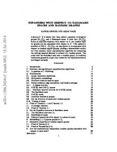
We need to complete the trimmed portion of antennai+1 (q) into a full antenna in Hi . Let v be one of these terminal points, lying in the intersection of all the hyperplanes pre-stored with the edge terminating at v, and in the new hyperplane that has cut the old antenna at v. Let f denote the intersection of all these hyperplanes. We then have to shoot within f , forward and backwards along some direction (say, a direction depending on ζ), until another hyperplane is hit, and keep doing so recursively, until a whole new portion of the antenna, “hanging” from v is constructed. See Figure 1. Repeating this completion process from all terminal vertices of the trimmed portion, we obtain the desired antennai (q).

p

Figure 1: The antenna of p in R3 . The structure of Mulmuley [25] has performed this antenna completion phase by preparing a recursive copy of the structure within each intersection flat f of any subset of the hyperplanes of Hi (for each i), with respect to the hyperplanes h ∩ f , for all h ∈ Hi not containing f . However, the overall input size of all these subproblems (not to mention their overall output size) is Ω(nd ), as is easily checked, which is too expensive for our goal. Schwarzkopf’s structure uses less storage, but it also maintains recursive (and rather complicated) substructures associated with lower-dimensional faces of the envelope. Instead, we only maintain the full-dimensional gradation-based structure, and perform each of the ray shootings in the antenna completion stage as if it were a new independent ray shooting query in d-space, Thus, on one hand we essentially ignore the extra information that the ray lies in some lower-dimensional flat, but on the other hand we do keep track of the dimension of the flat within which the current shooting takes place, so that we stop when we reach 0-dimensional features (vertices of the current LE(Hi )). Each of these recursive shooting steps starts again at Hk , and constructs the antenna by stepping backwards through the gradation. To speed up the query time, when we reach 3-dimensional flats, we switch to the data structures stored with the corresponding faces of LE(Hi ), and use them to perform the remaining shootings for the completion of the antenna. Analysis: Query time. Denote by Qj (n) the maximum expected cost of a query within a jdimensional flat, formed by the intersection of d − j of the given hyperplanes. We have Q3 (n) = O(log n). For j > 3 we argue as follows. We recursively obtain the antenna for the next set in the gradation, consisting of n/2 hyperplanes. Then we scan the conflict lists of the at most 2j vertices of the antenna, and find all the intersections of the hyperplanes in these lists with the antenna. We obtain various terminal points, lying on various lower-dimensional flats, and we recurse from each 17

of them within the corresponding flat. We thus obtain the recurrence X Qj (n) = Qj (n/2) + O(Cp ) + Qju (n),

(7)

u

where Cp is the sum of the sizes of the conflict lists of the vertices of the old antenna(p), and the sum is over the terminal points of the trimmed antenna, each with its own dimension ju (all strictly smaller than j). It follows from the theory of ε-nets that, with high probability, each of the conflict lists contains at most O(log n) hyperplanes, for a total of Cp = O(2j log n). In fact, as mentioned in the remark following Theorem 2.3 (with r = n/2), the expected sum of the sizes of these lists is only O(1). It is easy to verify by induction (on j and n) that the solution of (7) is Qj (n) = O(logj−2 n), so the cost of the original query, where j = d, is O(logd−2 n). Analysis: Storage and preprocessing. The maximum expected storage S(n) satisfies the recurrence S(n) = S(n/2) + O(n⌊d/2⌋ + C), (8) where C is the total size of the conflict lists of all the vertices of LE(H). A simple application of Theorem 2.3 shows that the expected value of C is O(n⌊d/2⌋ ), so, asymptotically, it has no effect on the recurrence (8), whose solution is then easily verified to be S(n) = O(n⌊d/2⌋ ). To bound the maximum expected preprocessing time T (n), we recall that most of it is devoted to the construction of the lower envelopes LE(Hi ), for i ≥ 0, and the conflict lists of all the vertices of each envelope; the time to construct the ray-shooting structures for all 3-dimensional faces is linear in the overall complexity of these facets, and is thus subsumed by the cost of the other steps. As described above, the construction of all the lower envelopes and the conflict lists of their vertices can be performed using the standard randomized incremental construction technique, whose expected running time is O(n⌊d/2⌋ ) for d ≥ 4, and O(n log n) for d = 3. The extra steps of copying envelopes and conflict lists at the appropriate prefixes do not increase the asymptotic bound on the running time. We have thus obtained the first main result of this section. Theorem 3.2. Given a set H of n hyperplanes in Rd , one can construct a data structure of expected size O(n⌊d/2⌋ ), so that, for any query point p ∈ Rd that lies below LE(H), and a query direction ζ, we can construct antenna(p) in H with respect to ζ in expected time O(logd−2 n). In particular, for any query ray ρ that emanates from a point below LE(H), we can find the point where ρ hits LE(H) (or report that no such point exists) within the same expected time. The expected preprocessing time is O(n⌊d/2⌋ ) for d ≥ 4, and O(n log n) for d = 3. Remark: The algorithm can be easily modified so that it can detect whether the query point p lies above LE(H). For this we take ζ to be the upward vertical direction (i.e., the xd -direction). In this case, the “bottom half” of antenna(p) (rooted at the segment that emanates from p downwards) does not exist, or alternatively consists of a single unbounded ray. When we pass from antennai+1 (p) to antennai (p), we scan the conflict lists of the vertices of the former antenna. If we find a hyperplane that passes below p, we stop the whole process and report that p lies above LE(H). Otherwise we continue as above. It is easy to verify the correctness of this procedure. Answering prefix-minima queries. We now return to our original goal, of using antennas to answer prefix-minima queries with respect to a random permutation π of the input hyperplanes. The pleasant surprise is that, with very few changes, the preceding algorithm solves this problem. 18

Specifically, as already described above, the gradation sequence H0 , H1 , . . . is constructed by taking each Hi to be the prefix of the first n/2i elements of π. We compute all the lower envelopes LE(Hi ) and the associated conflict lists using the technique described above, that is, by a single execution of the randomized incremental algorithm, using π as the insertion permutation. As above, we pause each time a full prefix Hi has been inserted (in the order i = k, k − 1, . . . , 0), and copy the current envelope and its conflict lists into our output. Given a query point q ∈ Rd−1 , we regard it as a point in Rd whose xd -coordinate is −∞, and construct the antennas antennai (q), with respect to the vertical shooting direction.5 Let e be the first edge of antennai+1 (q), incident to q and to some point on LE(Hi+1 ). While constructing antennai (q) from antennai+1 (q), we identify all hyperplanes of Hi \Hi+1 that intersect e, by collecting them off the prefixes of the appropriate conflict lists. We then scan these hyperplanes by increasing weight (i.e., rank in π), which is the order in which they appear in the conflict lists, and add each hyperplane h whose intersection with e is lower than all previous intersections to the sequence of prefix minima. By concatenating the resulting sequences, we obtain the complete sequence of prefix minima at q. The query time, storage, and preprocessing cost have the same expected bounds as above, and so we get the main result of this section. Theorem 3.3. Given a set H of n hyperplanes in Rd , and a random permutation π thereof, one can construct a data structure of expected size O(n⌊d/2⌋ ), so that, for any query point p ∈ Rd , the sequence of prefix minima of π among the hyperplanes intersecting the vertical line through p can be found in expected time O(logd−2 n). The expected preprocessing time is O(n⌊d/2⌋ ) for d ≥ 4, and O(n log n) for d = 3. Remarks: (1) Theorem 3.3 has Corollaries analogous to Corollaries 2.8 and 2.9 of Theorems 2.6 and 2.7, which we do not spell out. (2) The reason for including the antenna-based data structure in this paper is its elegance and simplicity (and also because of its applicability to point location and ray shooting below a lower envelope, providing a simple alternative to Schwarzkopf’s structure). It is easy to implement— both the preprocessing stage and the procedure for answering queries. Although we have not implemented the algorithm, we suspect that it will behave well in practice, and will outperform the theoretically more efficient cutting-based approach of Section 2. Experimentation with the algorithm might reveal that in practice the bound O(logd−2 n) on the expected query time is overpessimistic, and that its actual performance is much better on average.

4

Approximate Range Counting

In this section we exploit the machinery developed in the preceding sections, to obtain efficient algorithms for the approximate half-space range counting problem in Rd . Recall that in this application we are given a set P of n points in Rd , which we want to preprocess into a data structure, such that, given a lower halfspace h− bounded by a plane h, we can efficiently approximate the number of points in P ∩ h− to within a relative error of ε, with high probability (i.e., the error probability should go down to zero as 1/poly(n)). ¡ ¢ As explained in the introduction, following the framework of Cohen [9], we construct O ε12 log n copies of the data structure provided in Corollary 2.8, each based on a different random permutation of the points, obtained by sorting the points according to the random weights that they are assigned 5

Here we do not need the “bottom half” of the antenna, which is empty anyway.

19

from the exponential distribution (see the introduction and [9] for details).6 We now query each of the structures with the normal ω to h pointing into h− . From the sequence of points that we obtain we retrieve, in O(log n) time, the point of minimum rank in P ∩ h− , and record its weight. We output the reciprocal of the average of these weights as an estimator for the desired count. The preceding analysis thus implies the following results. Because of slight differences, we consider separately the cases d ≥ 4 and d = 3.

Theorem 4.1. Let P be a set of n points in Rd , for d ≥ 4. We can preprocess P into a data structure of expected size O( ε12 n⌊d/2⌋ log2−⌊d/2⌋ n), in O( ε12 n⌊d/2⌋ log2−⌊d/2⌋ n) expected time, so that, for a query halfspace h− , we can approximate |P ∩ h− | up to a relative error of ε, in O( ε12 log2 n) expected time, so that the approximation is guaranteed with high probability. In R3 we can reduce the storage using the following technique. ¢Let P be the given set of n ¡ points in R3 . Consider the process that draws one of the O ε12 log n random permutations π of P . Let R denote the set of the first t = ε2 n/ log n points in π. Clearly, R is a random sample of P of size t, where each t-element subset is equally likely to be chosen. Moreover, conditioned on R having a fixed value, the prefix πt of the first t elements of π is a random permutation of R. We now construct our data structure of Corollary 2.8 for R and ¡ 1 πt only. ¢ The expected size of 2 this data structure is O(t) = O(ε n/ log n). Repeating this for O ε2 ¡log n permutations, the total ¢ expected storage is O(n). The total expected construction cost is O ε12 log n · t log t = O(n log n). A query half-space h− is processed as follows. For each permutation π and associated prefix R, we find the point of R of minimum rank that lies in h− . If there exists such a point, it is also the minimum-rank point of P ∩ h− and we proceed as above. Suppose however that R ∩ h− = ∅. In this case, since R is a random ¢ of ¡P of size ¢t, the ε-net theory [16] implies that, with ¡ sample high probability, |P ∩ h− | = O nt log t = O ε12 log2 n . In this case, we can afford to report the ¢ ¡ points in P ∩ h− in time O ε12 log2 n , using the range reporting data structures mentioned in the introduction. For example, the algorithm of Chan [6] uses O(n log log n) storage, ¢log n) ¡ 1 O(n 2 − preprocessing time, and reports the k points of P ∩ h in time O(log n + k) = O ε2 log n . We then count the number of reported points exactly, by brute force. We proceed in this way if R ∩ h− is empty for at least one of the samples R. Otherwise, we correctly collect the minimum-rank elements in each of the permutations, and can obtain the approximate count as above. In summary, we thus have: Theorem 4.2. Let P be a set of n points in R3 , and let ε > 0 be given. Then we can preprocess P into a data structure of expected size O (n log log n), in O (n log n) expected time, so that, given a − − query halfspace ¡ 1h , 2we ¢can approximate, with high probability, the count |P ∩ h | to within relative error ε, in O ε2 log n expected time.

We note, though, that the structure of Afshani and Chan [1] gives a better solution. Remark: The same technique applies to the problem of approximate range counting of points in a query ball in Rd−1 , using the lifting transform, as described earlier. We obtain analogous theorems to Theorems 4.1 and 4.2, using Corollary 2.9; we omit their explicit statements.

References [1] P. Afshani and T. M. Chan, On approximate range counting and depth, Proc. 23rd Annu. ACM Sympos. Comput. Geom., 2007, 337–343. 6

To get the best asymptotic bounds, we use the data structure of Section 2, instead of the antenna-based one, but the latter structure can of course also be used.

20

[2] B. Aronov and S. Har-Peled, On approximating the depth and related problems, Proc. 16th Annu. ACM-SIAM Sympos. Discrete Algo., 2005, 886–894. [3] B. Aronov and S. Har-Peled, On approximating the depth and related problems, 2006, submitted. [4] B. Aronov, S. Har-Peled and M. Sharir, On approximate halfspace range counting and relative epsilon-approximations, Proc. 23rd Annu. ACM Sympos. Comput. Geom., 2007, 327–336. [5] B. Aronov and M. Sharir, Approximate range counting, Manuscript, 2007. [6] T. M. Chan, Random smapling, halfspace range reporting, and construction of (≤ k)-levels in three dimensions, SIAM J. Comput. 30 (2000), 561–575. [7] B. Chazelle, The Discrepancy Method, Cambridge University Press, Cambridge, UK, 2000. [8] K. Clarkson and P. Shor, Applications of random sampling in computational geometry, II, Discrete Comput. Geom. 4 (1989), 387–421. [9] E. Cohen, Size-estimation framework with applications to transitive closure and reachability, J. Comput. Syst. Sci. 55 (1997), 441–453. [10] M. de Berg, M. van Kreveld, M. Overmars and O. Schwarzkopf, Computational Geometry: Algorithms and Applications, 2nd edition, Springer Verlag, Heidelberg, 2000. [11] D. P. Dobkin and D. G. Kirkpatrick, Determining the separation of preprocessed polyhedra — A unified approach, proc. 17th Internat. Colloq. Automata, Languages and Programming, 1990, 400–413. [12] H. Edelsbrunner, Algorithms in Combinatorial Geometry, Springer-Verlag, Heidelberg, 1987. [13] H. Edelsbrunner and R. Seidel, Voronoi diagrams and arrangements, Discrete Comput. Geom. 1 (1986), 25–44. [14] L. Guibas, D. E. Knuth, and M. Sharir, Randomized incremental construction of Voronoi and Delaunay diagrams, Algorithmica 7 (1992), 381–413. [15] S. Har-Peled and M. Sharir, Relative ε-approximations in geometry, manuscript, 2006. (Also in [4].) [16] D. Haussler and E. Welzl, Epsilon-nets and simplex range queries, Discrete Comput. Geom. 2 (1987), 127–151. [17] H. Kaplan, E. Ramos and M. Sharir, The overlay of minimization diagrams during a randomized incremental construction, Manuscript, 2007. [18] H. Kaplan and M. Sharir, Randomized incremental constructions of three-dimensional convex hulls and planar voronoi diagrams, and approximate range counting, Proc. 17th Annu. ACMSIAM Sympos. Discrete Algo., 2006, 484–493. [19] Y. Li, P. M. Long, and A. Srinivasan, Improved bounds on the sample complexity of learning, J. Comput. Syst. Sci. 62 (2001), 516–527. [20] J. Matouˇsek, Reporting points in halfspaces, Comput. Geom. Theory Appl. 2 (1992), 169–186. 21

[21] J. Matouˇsek, Efficient partition trees, Discrete Comput. Geom. 8 (1992), 315–334. [22] J. Matouˇsek, Range searching with efficient hierarchical cuttings, Discrete Comput. Geom. 10 (1993), 157–182. [23] J. Matouˇsek and O. Schwarzkopf, On ray shooting in convex polytopes, Discrete Comput. Geom. 10 (1993), 215–232. [24] P. McMullen, The maximum numbers of faces of a convex polytope, Mathematika 17 (1970), 179–184. [25] K. Mulmuley, Computational Geometry: An Introduction Through Randomized Algorithms, Prentice Hall, Englewood Cliffs, NJ, 1994. [26] O. Schwarzkopf, Ray shooting in convex polytopes, Proc. 8th Annu. ACM Sympos. Comput. Geom., 1992, 886–894.

22