However, if code durations or onset and offset times were considered important, the ...... are saved in the HTML code, making the images mouse sensitive.
Behavior Research Methods 2008, 40 (I), 21-32
doi: 10.3758/BRM.40.1.2 I
RAP: A computer program for exploring similarities in behavior sequences using random projections VICENC QUERA
Universidad de Barcelona, Barcelona, Spain A computer program (RAP, for random projection) for exploring similarities between and within sequences of behavior is presented. Given a time window of a sequence, the program calculates a signature, a real-valued vector that is a random projection of the contents of the window (i.e., the codes occurring within it and their relative location, or onset and offset times) into an arbitrary K-dimensional space. Then, given two different time windows from the same sequence or from different sequences, their similarity is computed as an inverse function of the Euclidean distance between their respective signatures. By defining moving (overlapped or not overlapped) windows along each sequence and calculating similarities between every pair of windows from the two sequences, a map of similarities or possible recurrent patterns is obtained; the RAP program represents them as gray-level lattices, which are displayed as mouse-sensitive images in an HTML file. Computation of similarities is based on the random projection method, as presented by Mannila and Sepplinen (2001), for the analysis of sequences of events. The program reads sequence data files in Sequential Data Interchange Standard (SDIS) format (Bakeman & Quera, 1992, 1995a).
A pattern in a behavior sequence exists when there tend to be identical or similar repetitions of certain portions of it, which makes it possible to predict future behaviors from past ones, within some probability interval. Common methods for detecting such patterns include the fitting of Markov models in continuous and discrete time (e.g., Gardner 8 Hartmann, 1984), survival analysis in continuous tinie (e.g., Griffin & Gardner, 1989; Stoolmiller & Snyder, p006), lag-sequential analysis (e.g., Bakeman, 1978; Bakeman & Quera, 1995a; Sackett, 1979), log-linear model fitting to multidimensional contingency lag tables (e.g., Bakeman, Adamson, & Strisik, 1995; Bakeman & Quera, 1995b), and, more recently, analysis of sequence organization based on proximity coefficients among behavioral codes (Taylor, 2006). What these methods have in common is (1) the aim of summarizing relationships in the sequences by means of quantitative global measures, and (2) the use of asymptotic statistical techniques for obtainingp values that indicate whether or not the sequences contain patterns, and for pointing to statistically significant temporal relationships among behavioral codes. Alternative methods for the analysis of sequences have been developed that provide information about similarities within or between sequences, and many of them allow for visual exploration of possible patterns as well. These methods can be viewed as complementary to those described above, since it is usually highly advisable to explore the sequences of behavior for possible patterns
before carrying out an analysis based on inferential statistics. Methods that search for similarities and repetitions in sequences abound in biological sequence analysis, which consists mainly of aligning nucleotide sequences by means of dynamic programming algorithms (e.g., Durbin, Eddy, Krogh, & Mitchison, 1998); these algorithms have also been applied when researchers have been searching for similarities between sequences of sociological events (Abbott & Barman, 1997), aligning action protocols collected in human—computer interaction settings (Fu, 2001), and calculating observer agreement for event sequences (Quera, Bakeman, & Gnisci, 2007). Specific algorithms have been proposed for searching for repeated patterns in the analysis of interactive behavior (T-patterns, Theme software; Magnusson, 2000), in genomic analysis (maximal repeats, REPuter software; Kurtz et al., 2001), and in the data mining of sequences of alarms in telecommunication networks (e.g., Mannila & Toivonen, 1996; Moen, 2000). The use of dynamic-programming algorithms and repetition-searching algorithms in both cases requires extensive calculation; the former have the advantage ofproviding optimal alignments between sequences (i.e., alignments that minimize disagreements between them), whereas some of the latter (specifically, Theme and REPuter) yield visual displays indicating where patterns occur in the sequences being compared. Mannila and Seppfinen (2001) proposed a method for exploring repetition of similar situations
V. Quera, vquera®ub.edu
21
Copyright 2008 Psychonomic Society, Inc.
22
QUERA
(i.e., similar temporal organization of codes) in sequences of alarms in telecommunication networks. It is based on representing each code by a random vector in a space of an arbitrary number of dimensions and then defining time windows in the sequences and representing them by vectorial functions of the codes occurring within them and their relative locations; finally, Euclidean distances between the points representing the windows are computed. A similar method is used for calculating the distance between genes (e.g., Kang, 2005). When a certain number of codes are represented by random points in a space of arbitrary dimensions, it is said that codes are randomly projected into that space; if the number of dimensions of the space is lower than the number of codes, a dimensionality reduction is carried out. A dimensionality reduction is a powerful technique used in the analysis of multidimensional data that aims to represent a great number of variables by a subset of variables while capturing as much of the variation in the original data as possible. Applications of random projection include image and text processing (Achlioptas, 2003; Bingham & Mannila, 2001; Sahlgren, 2005), machine learning (Blum, 2006), and data mining in general. Although the most common purpose of random projection is reducing dimensionality while preserving essential properties of the data, "another, perhaps less intuitive scenario, is when projection to a lower-dimensional space actually highlights essential properties" (Vempala, 2004, p. 4). In this case, the purpose of using random projection to compute similarities between time windows in sequences is to highlight the parts of the sequences that tend to repeat and, thus, to highlight where patterns can probably be found. In this article, a program is presented that computes similarities among sections defmed in two sequences of behavior, according to the method outlined by Mannila and Seppänen (2001), and displays them as cells in a rectangular lattice, using gray levels to indicate degrees of similarity; this kind of graph is similar to the one used in dot matrix methods to explore similarities between amino acid sequences in genome analysis (e.g., States & Boguski, 1991). The program reads sequences of behavior from a data file and displays similarity lattices for pairs of sequences specified by the user. The program is written in Borland C+ + and Delphi Pascal and runs on Windows systems. BEHAVIOR SEQUENCES The random projection (RAP) program accepts SDIS data files, a format for representing sequences of behavior that defines five types of data: event, state, timed event, interval, and multievent sequences (Bakeman, 2000; Bakeman, Deckner, & Quera, 2005; Bakeman & Quera, 1992, 1995a; Quera & Bakeman, 2000). Following is an overview of the first three data types. Let C be a coding scheme, C = {c 1 c2 , , cm}, where ci is a code representing a discrete behavioral state and M is the number of different mutually exclusive and exhaustive (ME&E) codes. For example, in a study on joint attention during adult-infant interaction, the infant's verbal behavior could be represented by this coding scheme (based on Mas, 2003): C = {0 (the infant utters an ono,
matopoeia), W (the infant utters a word), P (the infant utters a phrase), N (the infant does not respond)). Suppose that behavior was coded using this scheme and that only the order in which the codes occurred was considered relevant, but not their durations and onset times. During an observation session, an event sequence would have been obtained, S: s 1 s2 . . . s,,, where si are codes belonging to C and n is the length of the sequence—for example, S:WWPNWNON. However, if code durations or onset and offset times were considered important, the following timed sequence would have been obtained: S: s2,t2-u2 . . . s„,t„-u„, where dashes separate onset and offset times for each code (respectively, ti and ui), expressed in appropriate time units, and code s i 's duration is given by di = ui -ti . If the codes are ME&E, that is a state sequence in which the onset time for a code equals the offset time for the code that immediately precedes it (and therefore, t i .4. 1 > ti); total duration for sequence S equals d = u n - t1 —for example, S: W,0-2 W,2-3 P,3-6 N,6-15 W,15-17 N,17-28 0,28-29 N,29-41, where time units are seconds. Note that in a state sequence, only onset times for the codes are in fact necessary, and the offset time for the last code must be explicitly stated. If not all codes in C are mutually exclusive (i.e., some of them may occur simultaneously) or if they are not exhaustive (i.e., some time units have no codes assigned), they can be represented as a timed event sequence. In the example above, if infant gestural codes are included and code N is removed, the coding scheme could be C = {0, W, P, S (simple, or spontaneous, gesture), R (relational gesture), J ( joint gesture—e.g., pointing)). In fact, two separate coding schemes could be defmed for verbal and gestural behavior: C v = {0, W, P} and CG = {S, R, J}. Codes in each scheme are mutually exclusive, but gestures and verbal utterances are not, since they can occur simultaneously; also, since the infant may remain silent or not gesture during certain time periods, the codes are not exhaustive. An example of a timed event sequence based on these coding schemes is S: W,0-2 J,0-6 P,3-6 S,10-12 W,15-17 J,16-17 P,25-30. In the example, several codes may overlap in time. Therefore, in these cases, either 4 + ui or ti .fi > u1 In the example, W,0-2 and J,0-6 overlap for 2 time units, whereas J,0-6 and P,3-6 overlap for 3 time units. There are also three different time gaps during which no code occurs, from 6 through 10, from 12 through 15, and from 17 through 25. .
SIMILARITY BETWEEN TIME WINDOWS
In order to compute the similarity between two sections, or time windows, belonging to different sequences S i and S2, the program first represents each section by a point in a K-dimensional space; then it computes the distance between the two points and transforms it into a similarity measure by means of an appropriate function. The steps will be detailed in the following paragraphs. Mapping the Codes For each code ci in the coding scheme, a mapping vector p k(c i) with K dimensions is defmed, and its components are
EXPLORING SIMILARITIES IN SEQUENCES
23
Table 1 Two Alternative Sets of Mapping Vectors in 10 Dimensions for Six Infant Verbal and Gestural Behavioral Codes Code 1 2 3 4 5 6 7 8 9 10 O W P S R
O W P S R J
A. 10-Dimensional Coordinates, Gaussian Distribution 1.0972 0.9482 -1.6819 -0.6289 -0.2642 -0.2462 -0.1101 -2.2061 -0.8089 0.3262 -0.2128 0.4906 -0.6881 -2.3814 -0.2231 -1.2982 0.6998 -0.0371 0.8672 -0.9148 1.0315 -0.0886 0.8352 1.2860 0.9168 -0.5167 -1.9647 -0.2173 1.6315 -1.1443 -2.0327 0.8232 1.5112 -0.9692 -1.1082 -0.6330 -1.9665 -1.0093 -0.8230 1.2079 0.2854 0.9361 -0.3157 -0.4925 -0.3920 -1.0767 -0.5467 0.3619 0.5237 -1.7015 0.8646 0.6140 -0.7695 1.4214 0.2499 -0.4185 -0.3891 0.9090 -0.4800 -1.0040 B. 10-Dimensional Coordinates, Three-Valued Sparse Distribution 0.0000 -1.7321 0.0000 -1.7321 0.0000 0.0000 1.7321 -1.7321 0.0000 0.0000 0.0000 -1.7321 0.0000 1.7321 1.7321 0.0000 0.0000 -1.7321 0.0000 0.0000 0.0000 0.0000 0.0000 0.0000 0.0000 0.0000 1.7321 0.0000 -1.7321 0.0000 -1.7321 0.0000 -1.7321 0.0000 -1.7321 0.0000 0.0000 -1.7321 0.0000 0.0000 0.0000 -1.7321 0.0000 1.7321 -1.7321 0.0000 0.0000 -1.7321 0.0000 -1.7321 0.0000 -1.7321 0.0000 0.0000 -1.7321 1.7321 -1.7321 -1.7321 -1.7321 -1.7321
assigned random real values that are sampled from some distribution, as the Gaussian or unit normal distribution, with a mean of zero and a standard deviation of one. Vector components are coordinates in a K-dimensional space, and thus we say that codes are projected into that space, where each code is represented by one point. IfK < M, the projection reduces the dimensionality of the data. Table lA shows six mapping vectors in K = 10 dimensions for each of the codes in the infant verbal and gestural coding scheme; coordinate values were sampled from the normal unit distribution. For each code, the vector components define one point in a 10-D space. Other distributions are possible besides the normal unit one; Achlioptas (2003) proposed two sparse distributions: a distribution with only two possible values for the ranlom variable, x = +1 or -1, withp = 1/2; and a distribution with only three values, x = + 43, 0, or -43, with p = 11/6,2/3, and 1/6, respectively. The sparse distributions have the advantage of being computationally simpler than the normal one and still provide sensible results. Table 1B shows six mapping vectors in K = 10 dimensions, sampled from the three-valued sparse distribution for each code in the infant verbal and gestural coding scheme. As Bingham and Mannila (2001) indicate, vectors pt(c) are not linearly independent, and thus the projections are not orthogonal; however, obtaining orthogonal vectors is computationally expensive, and "in a high-dimensional space, there exists a much larger number of almost orthogonal than orthogonal directions. Thus, vectors having random directions might be sufficiently close to orthogonal" (according to Hetch-Nielsen, 1994; the quote is from Bingham & Mantilla, 2001, p. 246). .
Defining Time Windows
Two sequence locations are specified in sequences S 1 and S2, marking the onset of the two sections, and window width w is defmed. Both the locations and the width are expressed in either events or time units, depending on the SDIS data type. For example, given the following timed event sequences, S I : W,0-2 R,1-6 P,3-6 S,10-12 W,15-17 S,16-17 P,25-30
and S2: W,5-8 R,8-9 P,9-13 S,15-18 W,20-23 J,22-23
R,24-25 P,31-33,
we can define an arbitrary window for the first sequence starting at 8 and another window for the second one starting at 12, and set w = 25 time units. Window contents are thus V I : 8[S,10-12 W,15-17 S,16-17 P,25-30]33 and V2: 12[S,15-18 W,20-23 J,22-23 R,24-25 P,31-33]37, where square brackets enclose the window contents, and the onset and offset times of the windows are indicated outside the brackets; offset times are exclusive.
Computing Wmdow Signatures
A signature is computed for each time window by multiplying the components of the mapping vectors that correspond to each code occurrence within the window by a function of the relative locations of the codes; for window V; (i = 1,2), the kth coordinate is given by yak =± pk (si ) • f (t r uy ), ja.1 where the sum is over the R. code occurrences within the window V; (i = 1, 2), su is the jth code occurring in it, and to and are its onset and offset times. The signature is thus a K-dimensional, real-valued vector that identifies the contents of the window quantitatively; in other words, the signature is a point in a K-dimensional space representing the contents of the window. The choice of K is arbitrary; when it is increased, high similarities stand out and low ones tend to fade away. No guideline exists as to which is the best value of K (see below); a minimum of K = 5 or K = 10 would seem to be advisable (Mannila & Seppinen, 2001). In matrix form, the signature for window Vi is defmed as y, = M, • where y is the K X 1 signature vector, M 1 is a K X R matrix containing the components of the mapping vectors (rows) corresponding to each code occurrence within window V i (columns), and fi is an R X 1 vector whose components are projection functions.
24
QUERA
Y12
YI3 Y14
371 .:•-•
M I fl
YIS = Y16 Y17 Y18
YI9 _YI,10
-2.033 +0.823 +1.511 -0.969 -1.108 -0.633 -1.966 -1.009 -0.823 +1.208
-0.213 +0.491 -0.688 -2.381 -0.223 -1.298 +0.700 -0.037 +0.867 -0.915
Thus, from the mapping vectors shown in Table 1, the signature for window V I is given in the matrix above. Columns in matrix M I contain the mapping vectors for codes S, W, S, and P in the order in which they occur within window V I . A linear projection function (LPF) that takes into account the onset time can be used: f (t.Y,u..)= Y
T - t. K,'
,
(1)
where T is the window offset time. Choosing T as the window offset time is arbitrary. Other points, such as the window onset time, could be chosen instead. In any case, what matters is that for each code occurrence, the function returns a value representing the relative position of the code's onset time within the window. Equation 1 yields values that are greater than 0 and less than or equal to 1 (0 would indicate that the code occurs very near the window termination, whereas 1 would indicate that it occurs when the window starts). For example, for the occurrence W,15-17, the projection function yields (33 - 15)/25 = .72. The (transposed) signature y i for window V I equals [-3.075 +1.642 +2.190 -2.854 -1.640 -2.113 -3.271 -1.711 -0.170 +0.908].
-2.033 +0.823 +1.511 -0.969 -1.108 -0.633 -1.966 -1.009 -0.823 +1.208
+1.031 -0.089 +0.835 +1.286 +0.917 -0.517 -1.965 -0.217 +1.631 -1.144 -
f (10, 12) f (15,17) f( 16, 17) f (25, 30)_ -
2001), which weighs codes higher as their onset times approach the end of the window; the sequential orderprojection function (SPF),f(t y,:ty) = r, which simply assigns each code occurrence its sequential position r within the window and ignores its onset time; and the occurrence function, f(to uy) = 1, which weighs all codes occurring within the window equally and, thus, for which only the fact that a code occurs, but neither its sequential order nor its exact onset and offset times, is considered important. Computing Window Similarity Given the signatures for the two windows, the Euclidean distance between them is computed: D ( VI , V2 )= 4/(Yik Y2k )2 •
Likewise, in order to obtain the signature for window V2, a matrix M2 with R = 5 columns, one per code occurrence (S, W, J, R, P), and a vector f2 with five projection functions are necessary. The signature y2 is then [-1.019 +1.892 +0.436 -1.567 -0.961 -2.375 -2.244 -0.232 +0.241 -1.321]. Alternatively, a projection function taking code durations into account, and not only their onset times, could be used by applying LPF to every time unit when the code occurs-that is, f (t e tty )= 1(T
-
I w.
nmt,
Other possible projection functions are the exponential,
f(to u y) = exp[(T - ty)/w - 1] (Mannila & Sept:linen,
2
5
10
20
Space Dimension (K) Figure 1. Mean distances among three windows (V 1 ,V2, andV31 see the text), for space dimensions K = 2, 5, 10, and 20. For each K, mapping vectors were assigned random Gaussian coordinates 1,000 times independently, and distances were computed between the resulting window signatures. The top, middle, and bottom lines correspond to mean D(V 2 , V3), D(V2, V3), and D(Vt, V2), respectively; vertical segments indicate standard deviations.
EXPLORING SIMILARITIES IN SEQUENCES
Figure 2. Similarity lattices for two timed event sequences of infant verbal and gestural behavior, obtained using a Gaussian random projection with If = 10 dimensions. Window width was set to 15, and starting times to 5 for both sequences. (A) Linear projection function, with shift equal to 15. (B) Sequential order projection function, with shift equal to 15. (C) Linear projection function, with shift equal to 1 and, thus, overlapping successive windows. Codes and their onset times are shown for each sequence. Similarities between several different pairs of time windows are indicated.
25
26
QUERA
The distance between two windows with identical contents equals zero, whereas any differences regarding the code occurrences, their relative locations within the windows, or both (depending on the kind of projection function used) will increase the distance. Using LPF, the distance between the two previous windows is D(V I ,V2) = 4.235. Distances can be converted into similarity measures by means of an inverse function, such as G(V i ,V2) = exp[ -D(V i ,V2)]. The negative exponential function is particularly useful because it highlights small distances by transforming them into large similarities, whereas big distances are transformed into negligible similarities; moreover, the resulting similarities are bounded between 0 and 1. Two windows with identical contents have G = 1, whereas any differences make G decrease toward 0. The similarity between the two previous windows is, thus, G(V I ,V2) = exp( -4.235) = .014. Since the mapping vector coordinates are random values, resampling them will result in different window signatures. Therefore, the actual distances between windows are likely to vary if the mapping vectors are resampled. Figure 1 shows mean distances among three windows— V3: 55[J,50-52 R,53 P,60-70 S,69]80, and previous V i and V2—for different space dimensions (K = 2, 5, 10, and 20); for each K, mapping vectors were assigned random Gaussian coordinates 1,000 times independently, LPF was used, and distances were computed between the resulting window signatures. Mean distances increase when the dimensionality increases and consistently indicate that, on average, D(V i , V3 ) is greater than both D(V2 , V3 ) and D(V i , V2). However, the three distributions of distances largely overlap when K is low, as Figure 1 indicates. Percentages of cases in which D(V i , V3 ) > D(V2 , V3 ) > D(V i , V2) are 61.1%, 70.2%, 80.7%, and 87.4% for K = 2, 5, 10, and 20, respectively, whereas percentages of cases in which D(V i , V3 ) > D(V i , V2) > D(V2 , V3 ) are 31.4%, 28.7%, 19.3%, and 12.6%, respectively. Therefore, increasing the space dimensionality tends to remove overlapping and maintain the order of distances.
windows will be overlapped; (2) ifs = w, they will be concatenated and not overlapped; (3) if s > w, they will not be concatenated, and some regions in the target sequences will be skipped. However, the exploration of sequences does not need to be directional; that is, given two sequences of comparable durations, we may be interested in exploring which sections in the first sequence are similar to sections in the second one, and vice versa. Even more, the two sequences can be the same sequence, and we may want to explore which sections in it tend to repeat. More generally, given two sequences S i and S2 with total durations d i and d2 , window width w, and shift s, both much smaller than d i and d2 , and a starting time tp for sequence p (p = 1, 2), a total of np successive windows can be explored for sequence p whose onset times are tp, tp + s, tp + 2s, . tp + (np - 1)s within the sequence; therefore, in total, n i n2 similarities can be calculated. For example, given the following timed event sequences (where offset times are omitted when they equal the corresponding onset time plus one), S i : P,5-18 S,5 S,13-20 P,30-54 S,34-37 S,42-46 S,58-61 W,59-61
SIMILARITY LATTICES
In order to search for a defined pattern (a short-sequence S i with a total duration d i ) in a target sequence (a longer sequence S2 with a total duration d2 , where d i