Rapid Object Indexing and Recognition Using Enhanced Geometric ...

Rapid Object Indexing and Recognition Using Enhanced Geometric Hashing Bart Lamiroy and Patrick Gros ? GRAVIR { Imag & Inria Rh^one-Alpes, 46 avenue Felix Viallet, F-38031 Grenoble, France

Abstract. We address the problem of 3D object recognition from a single 2D image using a model database. We develop a new method called enhanced geometric hashing. This approach allows us to solve for the indexing and the matching problem in one pass with linear complexity. Use of quasi-invariants allows us to index images in a new type of geometric hashing table. They include topological information of the observed objects inducing a high numerical stability. We also introduce a more robust Hough transform based voting method, and thus obtain a fast and robust recognition algorithm that allows us to index images by their content. The method recognizes objects in the presence of noise and partial occlusion and we show that 3D objects can be recognized from any viewpoint if only a limited number of key views are available in the model database.

1 Introduction In this paper we address the problem of recognizing 3D objects from a single 2D image. When addressing this problem and when the objects to be recognized are stored as models in a database, the questions \Which one of the models in the database best ts the unknown image?" and \What is the relationship between the image and the proposed model(s)?" need to be answered. The rst question can be considered as an indexing problem, the second as a matching problem. Indexing consists in calculating a key from a set of image features. Normally similar keys correspond to similar images while dierent keys correspond to dierent images. The complexity of comparing images is reduced to the comparison of their simpler indexing keys. Comparing two keys gives a measure of global similarity between the images, but does not establish a one-to-one correspondence between the image features they were calculated from [12]. Although indexing techniques are fast, the lack of quantitative correspondences, makes this approach unsuited for recognizing multiple or partially occluded objects in a noisy image. Since the indexing result only establishes a weak link between the unknown image and a model, a second operation is needed to determine the quantitative relationship between the two. Common used relationships are the exact location ?

This work was performed within a joint research programme between (in alphabetical order) Cnrs, Inpg, Inria, Ujf

of the model in the image, the viewpoint form which the image of the model was taken and/or aspect of the model the unknown image corresponds to. They can be calculated by solving the matching problem. I.e. establishing a correspondence between the image and model features. Solving the matching problem, however, is an inherently combinatorial problem, since any feature of the unknown image can, a priori, be matched to any feature in the model. Several authors have proposed ways to solve the recognition problem. Systems like the one proposed in [4] use a prediction-veri cation approach. They rely on a rigidity constraint and their performance generally depends on the optimisation of the hypothesis tree exploration. They potentially evaluate matches between every feature of every model and every feature of the unknown image. Lamdan and Wolfson [11] rst suggested the geometric hashing technique, which was later extended in several ways [8, 5, 6, 1]. It assumes rigidity as well, but the search is implemented using hashing. This reduced a part the complexity. Its main advantage is that it is independent of the number of models, although it still potentially matches every feature of every model. It has several other drawbacks however. Other approaches include subgraph matching, but are of a high complexity because the rigidity constraint is relaxed. They rely on topological properties which are not robust in the presence of noise. As a result, hashing techniques were developed using topological properties [10], without much success. Stochastic approaches containing geometric elements [2, 14], or based on Markov models generally demand very strong modeling, and lack exibility when constructing the model database. Signal based recognition systems [13] usually give a yes-no response, and do not allow a direct implementation of a matching algorithm. Our approach builds on geometric hashing type of techniques. Classical geometric hashing solves for the indexing problem, but not for the matching problem however. The new method that we propose solves simultaneously for indexing and matching. It is therefore able to rapidly select a few candidates in the database and establish a feature to feature correspondence between the image and the related candidates. It is able to deal with noisy images and with partially occluded objects. Moreover, our method has reduced complexity with respect to other approaches such as tree search, geometric hashing, subgraph matching, etc. The method, called enhanced geometric hashing, introduces a way of indexing a richer set of geometric invariants that have a stronger topological meaning, and considerably reduce the complexity of the indexing problem. They serve as a key to a multi-dimensional hash table, and allow a vote in a Hough space. The use of this Hough transform based vote renders our system robust, even when the number of collisions in the hash table bins is high, or when models in the model base present a high similarity. In the following section we shall describe the background of our approach. We shall explain the dierent choices we made and situate them in the light of previous work. Section 3 gives a brief overview of our recognition algorithm. Sec-

tions 4, 5 and 6 detail the dierent parts of our algorithm while Sect. 7 contains our experimental results. Finally, we shall discuss the interest of our approach, as well as future extensions in the last section.

2 Background and Justi cation Our aim is to develop a recognition system based on the matching technique proposed in [8, 9]. We shall further detail this technique in section 4. It is a 2D2D matching algorithm that extensively uses quasi-invariants [3]. This induces that our recognition and indexing algorithm will be restricted to 2D-2D matching and recognition. We can easily introduce 3D information however, by adding a layer to our model database2 . Instead of directly interpreting 3D information, we can store dierent 2D aspects of a 3D model, and do the recognition on the aspects. Once the image has been identi ed, it is easy to backtrack to the 3D information. Since our base method uses geometric invariants to model the images, and since we want to index these images in a model base, the geometric hashing algorithm by Lamdan and Wolfson [11] seems an appropriate choice. The advantage of this method is that it develops a way of accessing an image database with a complexity O(n) that depends uniquely on the size n of the unknown image. Multiple inconvenients exist however. They are the main reason for which we developed a new method we call enhanced geometric hashing. In our method we kept the idea of an invariant indexed hash table and the principle of voting for one or several models. The similarity stops there however. The classical geometric hashing has proved to contain several weaknesses. Our approach solves them on many points.

{ Grimson, Huttenlocher and Jacobs showed in [7] that the 4-point ane in-

variant causes fundamental mismatches due to the impossibility to incorporate a correct error model. Another account for false matches is that the 4-point invariant, used in the classical geometric hashing method is far too generic, and thus, by taking every possible con guration all topological information of the objects in the image is lost. We reduce this incertainty and loss of topological information by using the quasi-invariants proposed in [3, 9]. Instead of just extracting interest points, and combining them to form ane frames, we use connected segments to calculate the needed quasi-invariants. The segments are more robust to noise and the connectedness constraint reduces the possibility of false matches, since it is based on a topological reality in the image. { The new type of quasi-invariants and the connectedness constraint add another advantage to our method. For a given image containing n interest points, the number of invariants calculated by Lamdan and Wolfson is about O(n4 ). In our method, the number of quasi-invariants mainly varies linearly

2

Model database will also be referred to as model base.

with the number of interest points and lines. We therefore considerably reduce the total complexity of the problem. { It is known that the performance of the classical geometric hashing algorithm decreases when the number of collisions between models increases. The main reason for this is that the voting process only takes into account the quantitative information the possible matches oer. There is no qualitative measure that would allow votes to be classi ed as coherent or incoherent. We introduce a measure of coherence between votes by using the apparent motion between the unknown image and the possible corresponding model that is de ned by the match (cf. Sec. 4). Basically, the matched quasi-invariants de ne a geometric transform. This transform corresponds to an n-dimensional point in a corresponding Hough space. Coherent votes will form a cluster, while incoherent votes will be spread out throughout the whole transformation space. This enhanced voting method will allow us a greater robustness during the voting process. { Our quasi-invariants are particularly well suited to describe aspects of 3D objects, since they vary in a controllable way with a change of viewpoint. It is therefore easy to model a 3D object by its 2D aspects. Storing these aspects in our model base will allow us to identify an object from any viewpoint.

3 The Recognition Algorithm In this section we present the global lay-out of our recognition system. We shall brie y address its dierent parts. More detailed information will be given in the following sections. From now on, we shall refer to the images in the model base as \models", while the unknown images to recognize will be simply referred to as \images". It is to be noted, however, that there is no a priori structural dierence between the two. The classi cation only re ects the fact that \models" correspond to what we know, and what is stored in the model base, while \images" correspond to what is unknown what we want to identify. The recognition algorithm can be separated in four steps. The rst step can be considered \o-line". This does not mean, however, that, once the model base constructed it cannot be modi ed. New models can be added without aecting the performances of the recognition algorithm, and without modi cation of the model base structure. 1. Setting up the Model Base and Vote Space. For all the models we want to be able to recognize, we proceed in the following way: we extract interest points and segments from the model image. These points and segments will provide the con gurations needed for the calculation of the quasi-invariants. Once these invariants calculated we label them with the model from which they originated, and add them to the model base. Each model added to the model base also de nes a transformation space, ready to receive votes. 2. Extracting the necessary invariants from the unknown image. 3. Confronting Invariants with the Model Base. We calculate the needed invariants from an unknown image, and need to nd the models which are

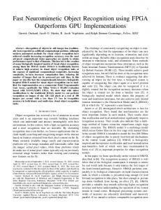
likely to correspond to it. As in the classical geometric hashing technique, the complexity of this operation is completely independent of the number of models or invariants present in the current model base. Every invariant of the image having been confronted to the model base, we obtain an output list containing the possible matches between image and the model features. The information contained in one element the output list consists of an invariant of the unknown image Ii , its possible corresponding invariant in one of the models Jjm , and the model to which Jjm belongs: Mm . 4. Voting in the Transformation Space. The output list obtained from the previous step, contains enough information to calculate an apparent motion between the unknown image and the corresponding model for each found match. This transform de nes a point in the transformation space, and due to the properties of the quasi-invariants, we know that coherent votes will form clusters, while unrelated votes will spread out in the vote space. The best model will be the one with the highest density cluster in its transformation space. Unknown Image

Extracted Invariants Model Base

Invariant Match Candidates I1 J1 M1 I1 J2 M2 I2 J3 M2

Vote Space M2

Hough Space 1 Hough Space 2

M3

Hough Space 3

Mn

Hough Space n

M1

Corresponding Model

In Jk Mj

Fig. 1. Object Recognition Algorithm: We extract the invariants of the un-

known image and feed them to the model base. The model base returns possible matches, which are used to calculate the transforms in the vote space. These transforms are added in the corresponding transformation space. The model presenting the best density cluster is returned as a match for the image.

4 Matching Invariants In this section we address the matching algorithm which our system is built on [8]. It was initially designed for image to image matching, but as we will show, it can easily be used to match an image to a model base. The principle is to calculate the invariants of n models, as well as those of an unknown image i. By comparing the invariants of the n models to those of i, and by using a voting technique, we can determine the model image that most resembles i.

4.1 Single Image to Image Matching

The base algorithm calculates quasi-invariants from features in an image. Quasiinvariants vary in a controllable way under projective transforms and are explicitly described in [3]. Since they vary only slightly with a small change in the viewpoint, they are well suited as a similarity measure between two con gurations. As shown in [3], the couple (; ) formed by the angle  and the length ratio  de ned by two intersecting segments, form a quasi-invariant. Moreover, these values are invariant under any similarity transform of the image. Gros [9] showed that it is valid to approximate the apparent motion between two images of a same object by such a similarity transform3 in order to obtain a match between the two. If we consider the con gurations of intersecting segments in two images of the same object (taken from dierent viewpoints, but with a camera movement that remains within reasonable bounds) the invariants of two corresponding con gurations should not dier too much. Matching these con gurations can be done is a two-stage process. We consider any pair of invariants that are not too dierent from one another. Hence, the corresponding con gurations are similar, and form a possible match. This gives us a list of possible matches between the two images. In order to determine which of them correspond to correct matches, we approximate the apparent motion between the two images by a similarity transform. Each possible match de nes such a transform, and allows us to calculate its parameters [8]. If we present each calculated similarity as a point in the appropriate transformation space, a correct match should de ne a similarity close to those de ned by the other correct ones, while incorrect matches will uniformly spread out in the transformation space. In the second stage, we therefore only need to search the four dimensional Hough space. We refer to this Hough space as \transformation space". The point with the highest density cluster wields the best candidate for the apparent motion between the two images. The invariant pairs having contributed to this cluster are those that give the correct matches between con gurations. (A weight can be aected to the votes, depending on the con dence and/or robustness accorded to both con gurations.) 3

By taking a dierent form of invariants, one can approximate the apparent motion by an ane transform [9]. We shall be using the similarity case, keeping in mind that the ane case could be applied to our method without loss of generality.

4.2 Single Image to Multiple Image Matching In order to match the invariants of one image i to those of the models in a model base, we could proceed by matching i to every model in the model base. As we have mentioned in the introduction, this operation is of too high a complexity. Since we aim at rendering the comparison phase independent of the number of models, we need to store our invariants in such a way that comparison only depends on the number of invariants in i, and not on the number of stored models in our model base. By using the values of the invariants as indexing keys in a multi-dimensional hash table we achieve the requested result. When we compare our invariants to the model base (as will be described in Sect. 5) the list of possible matches will be similar to the one obtained in the single image matching case. The only dierence is that the found matches will no longer refer to one model, but to various models present in the model base. By assigning a transformation space to each of the found models, we can vote in an appropriate transformation space for every possible match. Unlike Lamdan and Wolfson, we do not select the model having obtained the highest number of votes, but the one having the highest density cluster. By doing this we found an elegant way of ltering the incoherent votes from the correct ones, and we obtain a very robust voting system. Furthermore, the density cluster allows us to solve the matching problem, since it contains the invariant pairs that correctly contributed to the vote.

5 Storing Model Invariants and Accessing the Model Base Now that we have de ned the matching context, we can take a look at the way of easily store model invariants and allow a fast comparison with the image invariants. It has been shown [1, 6] that hash tables behave in an optimal manner when the keys are uniformly spread over the indexing space. Given a segment (on which we specify an origin O), however, a random second segment (with O as origin) will give a distribution of quasi-invariants (,) that is not uniform. In order to obtain an optimal use of the table entries and minimize the risk of losing precision within certain zones, we need to transform our initial invariant values to obtain a uniform probability. The distribution of the rst member of the invariant, the angle , is uniform, but it is not practical to compare two values in the [0; 2[ range since they are de ned modulo . By systematically taking the inner (i.e. smaller) angle between two segments, we obtain values within the [0; [ range. They conserve the property of uniform distribution and make comparison easier. We can solve the problem of the non-uniform distribution of the length ratio  in a similar fashion. Instead of considering the value  = ll21 , which has a non uniform distribution, we can use 0 = ln () = ln (l1 ) ? ln (l2 ) which behaves correctly as indexing key.

Now that we have solved the indexing problem, we can put the model invariants in our hash table. Since invariants contain noise and since their values are only quasi-invariant to the projective transforms that model the 3D-2D mapping, it is necessary to compare the invariants of the image to those in the model base up to an ". To compare an unknown invariant to those in the model base, we can proceed in any of the two following manners: { Since " is known at construction time, multiple occurrences of one invariant can be stored in the model base. To be assured that an invariant spans the whole "-radius incertainty circle4 we can store a copy of it in each of the neighbouring bins. At recognition time we only need to check one bin to nd all invariants within an " radius. { We can obtain the same result by storing only a single copy of the invariants. At recognition time however, we need to check the neighbouring bins in order to recover all invariants within the " scope.

6 Voting Complexity Voting in the vote space is linear in the number of found initial match candidates. The number candidates depends on the number of hits found by the model base. Their quantity is a function of the number of bins in the model base, and the number of models contained therein. Given an invariant of the unknown image, the probability to hit an invariant of a model in the model base varies linearly with the number of models. This probability also depends inversely on the number of bins and the distribution of the models in the model base. Basically, the complexity of the voting process is O (n  m). Where n is the number of invariants in the image and m the number of models in the model base.

7 Experimental Results In this section we present the results of some of the experiments we conducted on our method. The rst test, using CAD data, shows that our method allows us to correctly identify the aspect of a 3D object. A second test with real, noisy images, validates our approach for detecting and recognizing dierent objects in a same image.

7.1 Synthetic Data: Aspect Recognition We present here an example of 3D object recognition using aspects. We placed a virtual camera on a viewing sphere, centered in an L shaped CAD model, 4

As a matter of fact " is a multidimensional vector, de ning an uncertainty ellipsoid. For convenience we'll assume that it is a scalar de ning \"-radius incertainty circle". This aects in no way the generality of our results.

and took about 200 images from dierent angles. These images were used to automatically calculate 34 aspects that were fed into the model base. We then presented each of the 200 initial images to our recognition system5 . Since we have the program that generated the aspects at our disposal, we could easily check for the pertinence of the results given by our system. The results we obtained can be categorized in three groups: direct hits , indirect hits and failed hits . Direct hits are the images our system found the corresponding aspect for. Failed hits are those the system misinterpreted and attributed a wrong aspect. The indirect hits need some more attention and will be de ned below. In order to easily understand why indirect hits occur, we need to detail how the algorithm we used, proceeds in calculating the dierent aspects. The program uses a dissimilarity measure between images. In function of a dynamic threshold it constructs dierent classes of similar images. It is important to note that each image can belong to only one unique class. Once the dierent classes obtained, the algorithm synthesises all of the members of a class into a new \mean" view. This view is then used as the representative of this class. It is the combined eect of having an image belong to only one class, and synthetically creating a representative of a class that causes the indirect hits . It is possible that some of the members of other classes are similar to this synthesized view, although they were too dissimilar to some of the class members to be accepted in that class. One of the cases where this is situation is common, is when the algorithm decides to \cut" and start a new class. Two images on either side of the edge will be very similar, while their class representatives can dier allot. indirect hits do not necessarily occur systematically on boundaries however. The example in Fig. 2 (top) shows this clearly. We therefore de ne these hits as indirect since they refer to a correct aspect (in the sense that it is the one that corresponds to the best similarity transform), although it is not the one initially expected. They are considered as valid recognition results. As for the failed hits, we have noted that most come from degenerate views (cf. example in Fig. 2 bottom). Since we took a high number of images from all over the viewing sphere we necessarily retrieved some views where some distortion occurred. In the cited example, for instance, the \correct" model is the middle one. Our recognition algorithm proposed the model on the right for a simple reason: the distorted face of both the right model and the image are completely equivalent and dier only by some rotation, and the calculated \correct" model is a complete degenerate view that contains almost zero information. We obtained the following results for the recognition of our images: 5

In a rst time we presented the 34 aspects to the model base to check whether the system was coherent. We got a 100% recognition rate. Moreover, this result has been observed in all cases where the images our system was to recognize, had an identical copy in the model base. This result is not fundamental, but proves that the implementation of the dierent parts is sound.

Example of an indirect hit : the unknown image should have been assigned to the rst model. Our system matched it with the right model. As a matter of fact, the right model and the image only dier by a 114 rotation which is a better similarity transform than the one that approximates the apparent notion between the image and the other aspect. Example of an failed hit : the unknown image should have been assigned to the rst model. Our system matched it with the right model. The reason for this mismatch is due to the lack of information in the middle model, and the similarity between the two distorted lower faces.

Unknown Image

Aspect it should find

Recognition Result

Unknown Image

Aspect it should find

Recognition Result

Fig. 2. Examples of recognition results. # Models # Images Direct Indirect Failed Recognition Rate 34 191 151 (79.0%) 26 (13.6%) 14 (7.3%) 92.6% Without Hough vote: 36 correct hits 18.8%

7.2 Real Data: Object Recognition We shall now present the tests using real images containing noise. We took the image database of 21 objects from [10]. We then presented the a series of real images to the model base, containing one or more objects. Note that the image base is incomplete for our standards, since we don't have a complete series of aspects for the objects at our disposal. This will allow us to verify the behaviour of our method when unknown aspects or objects are present in an image. Some of the 16 images we used to test recognition algorithm can be found in Fig. 3. We conducted two types of tests: rst we tried to detect one object per image for all images; in a second stage we asked our system to recognize the number of objects we knew were present in the image. We obtained a 94% recognition rate for the rst kind of tests ( rst three results in Fig. 3). The second series show that there are three types of images: those showing known objects in a known aspect, images showing known objects in an unknown aspect, and those featuring unknown objects. For the objects showing a known aspect we obtain a very good recognition rate (9 out of 11 objects are recognized). This con rms the eectiveness of our method. For the image containing no known objects we get excellent results as

Known objects in a known Unknown aspect objects

Known objects in an unknown aspect

Images

Invariants Output

Fig. 3. Some of the 16 images used for recognition. well: 6 models were matched ex aequo with a very low vote weight compared to the previous results. However, none of the matched objects with an unknown aspect was correct (last two results Fig. 3). Although this result may seem deceptive, we note that the weight of the votes resulting in the second match are signi cantly lower than those identifying a correct aspect. Furthermore, our system does not use any 3D information whatsoever. Recognition of unknown aspects from 3D objects does not fall within its scope, which we showed with this experiment.

8 Discussion and Future Extensions In this paper we presented a new solution to the problem of object recognition in the presence of a model database. We have developed an indexing technique we called enhanced geometric hashing. Our approach allows us to solve for the indexing and matching problem in one pass in a way similar to the geometric hashing approach and is able to detect and recognize multiple objects in an image. Other contributions consists in using invariants that contain more topological information and are more robust than the simple 4 point con guration, enhancing the voting phase by introducing a richer and more discriminating vote, and reducing the complexity of the problem. We validated our approach on both CAD and real image data, and found that our approach is very robust and ecient. Although it is based on 2D image information, we have showed that we can recognize 3D models through their aspects.

Medium term evolutions of our system may consist of: automatically nding multiple objects in one image, matching n images to each other instead of a single image to m models (This may prove extremely useful for the aspect calculating clustering algorithm), optimizing the voting process by precalculating parts of the ane transform or by using techniques of sparse distributed memory, extending the scope of invariants used, etc.

References 1. G. Bebis, M. Georgiopoulos, and N. da Vitoria Lobo. Learning geometric hashing functions for model-based object recognition. In Proceedings of the 5th International Conference on Computer Vision, Cambridge, Massachusetts, USA, pages 543{548. IEEE, June 1995. 2. J. Ben-Arie. The probabilistic peaking eect of viewed angles and distances with application to 3-D object recognition. Ieee Transactions on Pattern Analysis and Machine Intelligence, 12(8):760{774, August 1990. 3. T.O. Binford and T.S. Levitt. Quasi-invariants: Theory and exploitation. In Proceedings of Darpa Image Understanding Workshop, pages 819{829, 1993. 4. R.C. Bolles and R. Horaud. 3DPO : A three-Dimensional Part Orientation system. The International Journal of Robotics Research, 5(3):3{26, 1986. 5. A. Califano and R. Mohan. Multidimensional indexing for recognizing visual shapes. Ieee Transactions on Pattern Analysis and Machine Intelligence, 16(4):373{392, April 1994. 6. L. Grewe and A.C. Kak. Interactive learning of a multiple-attribute hash table classi er for fast object recognition. Computer Vision and Image Understanding, 61(3):387{416, May 1995. 7. W.E.L. Grimson, D.P. Huttenlocher, and D.W. Jacobs. A study of ane matching with bounded sensor error. In Proceedings of the 2nd European Conference on Computer Vision, Santa Margherita Ligure, Italy, pages 291{306, May 1992. 8. P. Gros. Using quasi-invariants for automatic model building and object recognition: an overview. In Proceedings of the NSF-ARPA Workshop on Object Representations in Computer Vision, New York, USA, December 1994. 9. P. Gros. Matching and clustering: Two steps towards object modelling in computer vision. The International Journal of Robotics Research, 14(5), October 1995. 10. R. Horaud and H. Sossa. Polyhedral object recognition by indexing. Pattern Recognition, 28(12):1855{1870, 1995. 11. Y. Lamdan and H.J. Wolfson. Geometric hashing: a general and ecient modelbased recognition scheme. In Proceedings of the 2nd International Conference on Computer Vision, Tampa, Florida, USA, pages 238{249, 1988. 12. H. Murase and S.K. Nayar. Visual learning and recognition of 3D objects from appearance. International Journal of Computer Vision, 14:5{24, 1995. 13. R.P.N. Rao and D.H. Ballard. Object indexing using an iconic sparse distributed memory. In Proceedings of the 5th International Conference on Computer Vision, Cambridge, Massachusetts, USA, pages 24{31, 1995. 14. I. Shimshoni and J. Ponce. Probabilistic 3D object recognition. In Proceedings of the 5th International Conference on Computer Vision, Cambridge, Massachusetts, USA, pages 488{493, 1995. This article was processed using the LaTEX macro package with ECCV'96 style