near-future event prediction by an online learning agent operating .... that can accurately sort out the context and learn that (C, A) pre- dicts 'B' with probability 1 ...
Rapid On-line Temporal Sequence Prediction by an Adaptive Agent Steven Jensen, Daniel Boley, Maria Gini, and Paul Schrater Department of Computer Science and Engineering University of Minnesota {sjensen,boley,gini,schrater}@cs.umn.edu
ABSTRACT Robust sequence prediction is an essential component of an intelligent agent acting in a dynamic world. We consider the case of near-future event prediction by an online learning agent operating in a non-stationary environment. The challenge for a learning agent under these conditions is to exploit the relevant experience from a limited environmental event history while preserving flexibility. We propose a novel time/space efficient method for learning temporal sequences and making short-term predictions. Our method operates on-line, requires few exemplars, and adapts easily and quickly to changes in the underlying stochastic world model. Using a short-term memory of recent observations, the method maintains a dynamic space of candidate hypotheses in which the growth of the space is systematically and dynamically pruned using an entropy measure over the observed predictive quality of each candidate hypothesis. The method compares well against Markov-chain predictions, and adapts faster than learned Markov-chain models to changes in the underlying distribution of events. We demonstrate the method using both synthetic data and empirical experience from a gameplaying scenario with human opponents.
Categories and Subject Descriptors I.2 [Artificial Intelligence]: Learning
General Terms Algorithms
Keywords Rapid Learning, sequence prediction, n-gram, Markov Decision Process
1. INTRODUCTION Robust sequence prediction is an essential capability for an intelligent agent interacting in a dynamic environment. By making accurate predictions, the agent is able to reduce the space of future events which, in turn, facilitates better decision making and
reduced planning, and permits multi-agent coordination without communication. In this paper we consider the case of an agent that must learn to make predictions on the fly while acting in a non-stationary environment. Making predictions under these conditions is quite challenging. Agents must learn rapidly in order to adapt to changes in event generating processes, limiting the amount of historical data that can be considered. Because the agent is operating while learning, the learning process must also be online and time/space efficient. Existing sequence prediction methods like HMMs are not designed for this problem. Most methods require the process to be stationary, with an abundance of data. Many learning methods (such as the EM algorithm) are better suited to offline learning. Thus, the challenge for a learning agent in a rapidly changing environment is to exploit the relevant experience while preserving flexibility. We propose a solution that employs short-term memory to rapidly store regularly occurring patterns in sequences of observations. These sub-sequences (representing candidate predictors) are filtered by finding those that produce high and reliable prediction performance. This solution is qualitatively similar to the human sequence prediction strategy suggested by recent research [6], in that humans appear to use a combination of short-term memory and the detection of apparent non-randomness in sensory input to rapidly learn regularly occurring patterns in sequences of observations. One of the key aspects of the proposed solution is to exploit basic, low-level predictability in temporal sequences. Low-level predictability can be modelled via a variable-length order-n Markov chain, where n is the number of consecutive observations needed to predict the next observation. Recall that the joint probability distribution of a sequence of observations o1:n = o1 , o2 , . . . , on can always be factored as P (o1 , o2 , . . . , on ) = P (o1 )
n Y
P (ot |o1:t−1 )
(1)
t=2
The full joint distribution becomes intractable as the sequence length increases, however a fixed finite length n Markov model P (oT −n+1 , . . . , oT )
T Y
P (ot |oT −n:T −1 )
t=T −n+1
Permission to make digital or hard copies of all or part of this work for personal or classroom use is granted without fee provided that copies are not made or distributed for profit or commercial advantage and that copies bear this notice and the full citation on the first page. To copy otherwise, to republish, to post on servers or to redistribute to lists, requires prior specific permission and/or a fee. AAMAS’05, July 25-29, 2005, Utrecht, Netherlands. Copyright 2005 ACM 1-59593-094-9/05/0007 ...$5.00.
is poorly suited to capture regularities with variable lags and multiple time scales. Our short-term memory approach extracts subsequences with variable lags, overcoming some of the problems of fixed length Markov chains. The results of this paper suggest that a machine learning approach that exploits basic, low-level predictability may overcome the problems introduced by online learning in a non-stationary environment.
2. A MOTIVATING EXAMPLE Consider the following situation in which a learning agent encounters the following sequence of observations: (for simplicity we denote an observation with a single upper case letter): ABACABAC A ? If an order-1 Markov assumption is made, then the model, when presented with the given sequence up to the final event A should predict the subsequent occurrence of the event ‘B’ or ‘C’ with equal probability. If we arbitrate with the flip of a coin, we can expect no better than 50% success at predicting the succeeding event. However, this is clearly not what a human observer would immediately induce from the same sequence. A human observer recognizes that events ‘B’ and ‘C’ alternate with regularity and are completely predictable. If we simply augment our definition of ‘state’ to include 2 consecutive events (order2 Markov chain), we have increased the number of possible states from 3 (A, B, or C) to 9 (AA AB . . . CC), but now we have a model that can accurately sort out the context and learn that (C, A) predicts ‘B’ with probability 1 and (B, A) predicts ‘C’ with probability 1. Increasing the order of the Markov chain is a common method for augmenting the definition of state in order to uncover predictable relationships in temporal sequences, however the drawback to this approach lies in the combinatorial explosion in the state space and in the large number of training samples needed for the agent to learn. This is problematic for an agent operating in a highly dynamic environment that must learn quickly with limited experience.
3. ELPH: ENTROPY LEARNING PRUNED HYPOTHESIS SPACE We propose an alternate method, using the notion of an actively pruned “hypothesis” space that is able to sort out highly predictive patterns regardless of the Markov order and do so with relatively few examples. The method avoids some of the pitfalls of current methods such as the need for long training sequences and uncontrollable combinatorial explosion, and provides rapid, online learning. Furthermore, it is capable of quickly adapting to pattern changes. We refer to the algorithm using the acronym ELPH (”Entropy Learning Pruned Hypothesis space”) Unlike order-n Markov chain methods, in which learning occurs over a space of uniform n-grams, this algorithm learns over a space of hypotheses, referred to as the Hypothesis Space (HSpace). Given a short-term memory consisting of the n most recent temporallyordered observations, an individual hypothesis consists of a subset of the ordered contents of the short-term memory of recent observations and an associated prediction-set of events that have, in the past, immediately followed the pattern contained in short-term memory. Consider some event et occurring at time t which is immediately preceded by a finite series of temporally ordered observations (ot−n , . . . , ot−1 ). Our task is to determine if some subset of those observations consistently precedes the event et . If such a subset exists, then it can be subsequently used to predict future occurrences of et from a temporally ordered set of observations. The question then becomes, “is this event consistently preceded by some specific pattern of observations?” In general, if the observed system takes the form of a Markov chain of order-1, then the single observation ot−1 will predict the probability of the event et . However, given an arbitrary series of observations, it is not necessarily true that the sequence results from a Markov process of order-1. For example, it may be that the single observation ot−4 accurately predicts the observed event while the
observation ot−1 is irrelevant. Or perhaps the two specific observations {ot−6 , ot−4 } predict the observed event with high probability, and so on. Assuming, without loss of generality, that we fix the length of the histories stored in the short-term memory to n = 7, we may either select or ignore each of the n = 7 observations in each history. This leads to 2n = 128 possible subsets of the recent event history that can be used to form hypotheses, equivalent to the power-set formed from the 7-gram short-term memory. If we disregard the trivial hypothesis (consisting only of the empty-set {}), then for any specific short-term memory configuration, we can form 127 individual hypotheses, each of which “may” have predicted the observed event at time t. The choice of n = 7 is arbitrary, and we could have selected a different value. The inspiration came from the work by Miller [7]. At each time step, the system attempts to learn which of the possible subsets is consistently good at predicting the current event et . It does this by adding a potential hypothesis for each possible subset of the observation history corresponding to the currently observed event, et : {ot−1 } ⇒ et {ot−2 } ⇒ et .. . {ot−6 , ot−4 } ⇒ et .. . {ot−7 , ot−6 , . . . , ot−1 } ⇒ et where et is the observation at time t that this rule is trying to predict. The exact process by which the HSpace is filled with these hypotheses is the learning process outlined next. By forming these hypotheses in real-time, we are able to learn those that, over time, predict specific events with high-probability and utilize them to make predictions of future events.
3.1
Learning
The HSpace is used to store the hypotheses encountered and generated from previous time steps. Associated with each hypothesis is its set of predictions together with counts for each prediction indicating how many times it has been encountered in the past. As each observation (or percept), o, is sensed, it is entered into a n-element short-term memory containing the recently observed history. The short-term memory is implemented as a fifo queue and is organized in a fixed temporal sequence: (ot−7 , ot−6 , ..., ot−1 ). At each discrete time step, t, a new set of 127 hypotheses is formed from the stored observations in the short-term memory, along with the currently observed event at time t. Each of the 127 individual hypotheses are then inserted into the hypothesis space subject to the following rules: 1. If the hypothesis is not in the HSpace, it is added with an associated prediction-set containing only the current event (prediction) and an event count set to 1. 2. If the hypothesis already resides in the HSpace, then the observed event is matched with the stored predictions in the associated prediction-set. If found, the proposed hypothesis is consistent with past observations and the event count corresponding to et is simply incremented. 3. If the hypothesis already resides in the HSpace but the observed event et is not found in the associated prediction-set, the novel prediction is added to the prediction-set with an event count of 1.
3.2 Pruning the hypothesis space The combinatorial explosion in the growth of the HSpace is controlled through a process of active pruning. Since we are only interested in those hypotheses that provide high-quality prediction, inconsistent hypotheses or those lacking predictive quality can be removed. Note that, for any given hypothesis, the prediction-set represents a histogram of the probability distribution over those events that have followed the specified pattern of observations. The entropy of this distribution is a measure of the prediction uncertainty and can be considered an inverse qualitative measure of the prediction. The prediction-set P S for each hypothesis in the HSpace consists of a set of ν tuples (ei , ci ), one for each of the ν events predicted by the hypothesis, P S = {(e1 , c1 ), (e2 , c2 ), . . . , (eν , cν )} where ci is the count of the number of times that ei followed this hypothesis’s list of observations in the data sequence. Using the individual event counts, the entropy of the prediction set can be computed as, H=−
ν X i=1
ci log2 ctot
�
ci ctot
�
contents of the short-term memory, and rank them according to entropy measure. The maximum number of matching hypotheses is bounded by the length of the short-term memory. With our choice of keeping the last n = 7 observations in the short-term memory, there are at most 127 such matching hypotheses. The most frequently occurring prediction (maximum likelihood) from the hypothesis with the lowest-entropy is the best prediction that can be made, given the current experience. For making predictions, a simple entropy computation is not sufficient because it is biased toward selecting those hypotheses with a small number of occurrences. For example, a hypothesis that has only occurred once will have a single prediction-set element, producing a computed entropy value of zero. A more robust entropy measure must be used that takes into account the number of occurrences and gives greater weight to those with higher frequency. A more reliable entropy measure is obtained by re-computing the prediction-set entropy with a single, false positive added to the set. We add a single, hypothetical false-positive element which represents an implicit prediction of ”something else”. This yields a reliable entropy measure, Hrel =
i=1
−
where ctot is simply the sum of all the individual event counts, ctot =
ν X
ci
i=1
If a specific hypothesis is associated with a single, consistent prediction, the entropy measure for that prediction-set will be zero. If a specific hypothesis is associated with a number of conflicting predictions, then the associated entropy will be high. In this sense, the “quality” of the prediction represented by the specific hypothesis is inversely related to the entropy measure. High entropy indicates poor predictive quality, and low entropy indicates consistently accurate prediction. As hypotheses are added to the HSpace, inconsistent hypotheses are removed. An inconsistent hypothesis is one in which the entropy measure over the prediction-set exceeds a predetermined threshold Hthresh . In other words, when the entropy measure of the predictions associated with a specific hypothesis is high, it fails the “predict with high probability” test and is no longer considered to be a reliable predictor of future events, so it is removed from the HSpace. It is this pruning behavior which bounds the growth in the hypothesis space. Over time, only those hypotheses deemed accurate predictors with high probability are retained. All others are eventually removed. Entropy threshold pruning also facilitates rapid adaptation in non-stationary environments. When the underlying process statistics change, the resultant increase in prediction-set entropy causes existing hypotheses to be removed and replaced by low-entropy hypotheses learned following the change.
3.3 Making predictions The hypotheses which are retained in the HSpace are generally high-quality predictors of future events and can be used to perform serial prediction tasks. These predictions are made by considering all hypotheses consistent with the current contents of the short-term memory and choosing the “most likely” hypothesis. Again, an entropy measure over the prediction-set can be used as a qualitative prediction measure: The lower the entropy, the “better” the prediction. To make a prediction, we simply locate the hypotheses in the HSpace which are represented by the current
−
"ν X
ci log2 ctot + 1
1 log2 ctot + 1
�
�
ci ctot + 1
1 ctot + 1
�#
�
If a specific hypothesis in the HSpace has only occurred once, its associated prediction-set will contain a single element with an event count of 1. This yields a computed prediction-set entropy of log2 (1) = 0.0. However, using the reliable entropy measure Hrel yields an adjusted entropy of − 21 log2 ( 12 ) − 21 log2 ( 12 ) = 1. Note that a prediction-set with a single element but a high event count will yield a reliable entropy considerably less than 1. In this case, the reliable entropy measure is consistent with the intuitive notion of “predictability” implied by frequent occurrence.
3.4
Brief analysis
For an alphabet of size m, an order-n Markov chain approach requires a transition matrix of dimension mn . The proposed ELPH algorithm spans a potential space of order (m + 1)n which is significantly larger. However, two attributes of the problem domain restrict the effective size of the HSpace: 1. Limited experience yields a sparse space: Only those hypotheses that both have been experienced and have high predictive quality are kept in the HSpace. 2. Statistical structure in the observation space leads to efficient pruning: If the temporal stream of observations is truly random, leading to no ability to predict future events, then the HSpace method will indeed explode, or in the presence of pruning, will continually prune and add new hypotheses (i.e. thrash). However, most interesting “real-world” behavior has regularities our algorithm should efficiently exploit.
3.5
An example
We show step by step how the HSpace is constructed in Table 1. The hypotheses are shown in the row of the corresponding observation. For this example, we restrict the amount of history in the short-term memory to n = 2 for illustration simplicity. Given the following input: ... A B A C A B A D ...
observation A B A C A B A D
hypotheses added ... ... AB BA AC CA AB BA
⇒ ⇒ ⇒ ⇒ ⇒ ⇒
{(A, 1)} {(C, 1)} {(A, 1)} {(B, 1)} {(A, 2)} {(D, 1), (C, 1)}
... ... ∗B ∗A ∗C ∗A ∗B ∗A
⇒ ⇒ ⇒ ⇒ ⇒ ⇒
... ... A∗ B∗ A∗ C∗ A∗ B∗
{(A, 1)} {(C, 1)} {(A, 1)} {(B, 1), (C, 1)} {(A, 2)} {(D, 1), (B, 1), (C, 1)}
⇒ ⇒ ⇒ ⇒ ⇒ ⇒
{(A, 1)} {(C, 1)} {(A, 2)} {(B, 1)} {(A, 3)} {(D, 1), (C, 1)}
Table 1: Operation of the ELPH algorithm on a short sample stream. The ‘*’ denotes an observation that is ignored. at the second occurrence of observation ‘A’ three hypotheses will be inserted in the HSpace: A* ⇒ A
* B ⇒ A,
where ‘*’ stands for an observation that is ignored. Following the subsequent observations ‘C’ and ‘A’, six additional hypotheses will be inserted, namely BA ⇒ C AC ⇒ A
B* ⇒ C A* ⇒ A
*A ⇒ C * C ⇒ A.
At the second occurrence of observation ‘B’, ‘*A’ predicts not only ‘C’, as before, but also ‘B’. We now have an ambiguous prediction, with ‘B’ being predicted with probability 21 and ‘C’ also being predicted with probability 21 . The entropy of the ‘*A’ prediction goes to 1. In the next time step, we observe ‘A’ and since ‘A*’ has predicted ‘A’ consistently three times its reliable entropy decreases. In the next time step, we observe ‘D’ and now the ambiguity of ‘*A’ includes ‘D’, ‘B’, and ‘C’. The entropy of the prediction set of ‘*A’ has now increased to approximatively 1.5 and has become a good candidate for pruning.
Prediction accuracy (proportion correct)
AB ⇒ A
ELPH performance for a family of stationary processes 1 Ideal Markov Predictor ELPH ML Markov Learner
0.9
0.8
0.7
0.6
0.5
0.4
0.3
0.2
blind guess rate 0.1
0
0
0.5
1
1.5
2
2.5
Entropy rate of stationary process
Figure 1: ELPH performance on strings from increasingly stochastic processes. Prediction accuracy is compared to both an ideal Markov predictor and a maximum likelihood Markov learner on identical strings.
4. EXPERIMENTAL RESULTS We tested the ELPH algorithm on a series of synthetically generated strings derived from both stationary and non-stationary discrete stochastic processes. The performance was measured and compared to that of various Markov agents on prediction tasks in which each agent observed the input string one element at a time and predicted the subsequent element. The performance measure for all agents was the proportion of the number of correct predictions to the total number of elements in the input string.
4.1 Performance in stationary environments We constructed an order-1 Markov process to generate test data strings by taking the convex combination of two underlying Markov transition matrices, S1 and U , to form a new transition matrix A = (1 − λ)(S1 ) + (λ)(U ), 0 ≤ λ ≤ 1 The matrix S1 is representative of a nearly deterministic process in which the state transitions are set to a value approaching 1, but slightly less than unity to maintain the acyclic property (e.g. 0.9999). The second matrix, U , has state transition probabilities uniformly distributed throughout and is representative of a completely random process with maximal entropy rate. λ is used to control the entropy rate of the resulting Markov process. The dimension of the generating transition matrix was fixed at 5 throughout all trials reported. This Markov process was then used to generate strings of 1,000 elements each.
In Figure 1, ELPH performance is compared to both an ideal Markov predictor and a maximum likelihood Markov learner. Each sample point represents the prediction accuracy achieved on a synthetically generated string. We repeated the experiment 100 times, each time generating a 1000 length string from a stationary stochastic process and then systematically increasing the entropy rate of the generating process. The ideal Markov predictor is an agent that makes maximum likelihood estimates of the successor state directly from the generating transition matrix. The performance of the ideal predictor provides a baseline representative of the best prediction that can be made for any given discrete stochastic process. The maximum likelihood (ML) Markov learner is an agent that has no knowledge of the size of the state-space or generating transition matrix and must estimate these values from observations obtained on the fly. Given an observation history, the ML Markov learner observes a state and constructs the maximum likelihood of the successor state by accumulating observed state transitions over time. Figure 2 illustrates the performance of the ELPH algorithm when the length of context history is limited to 1 and the entropy threshold is set to a value which eliminates all pruning behavior. With no pruning and a history of length 1, the ELPH algorithm should be equivalent to a maximum likelihood Markov learner of order-1. As expected, the ideal Markov predictor performs better than all
4.2 Performance in non-stationary environments The series of tests illustrated in Figures 1 and 2 describe performance on strings generated from stationary processes. In these cases, adaptability is not an issue. To measure the adaptability of the ELPH algorithm compared to other methods, we created non-stationary processes by alternating between two mixture models with independent λ values. The first process (A) was created as described earlier, the second process (B) utilized a separate mixture coefficient λB and a different transition matrix S2 , formed by rotating the columns of S1 by 1. The time between model switches was specified by a duration parameter d, measured in samples. Non-stationary strings were created by alternating sampling from process A for a duration of d samples,
Equivalence of ELPH to ML in the absence of pruning 1
Prediction accuracy (proportion correct)
ELPH (history=1) ML Markov Learner 0.9
0.8
0.7
0.6
0.5
0.4
0.3
0.2
blind guess rate 0.1
0
0
0.5
1
1.5
2
2.5
Entropy rate of stationary process
Figure 2: Equivalence of ELPH to order-1 ML Markov learner when history is limited to 1 and entropy threshold is set to a high value disabling pruning.
and from process B for a duration of d samples. This method yielded strings in which the non-stationarity of the process could be altered by changing the rate at which generating process alternation occurred, or by altering the degree of randomness of either of the generating processes (or both). We performed two sets of experiments. For the first set, we systematically changed the rate of alternation of two highly deterministic generating processes and we measured the effect of the length of the history used by ELPH. For the second set of experiments, one of the generating processes was highly deterministic and the second was increasingly stochastic. We compared ELPH with a Markov learning process which used the same history length. All trials used transition matrices of dimension 5 with Hthresh set to 1.0. ELPH Performance on low entropy rate non−stationary processes 1
Prediction accuracy (proportion correct)
other methods tested and serves as a benchmark for optimal performance. Due to the fact that these are stationary strings of sufficient length to provide an adequate sample of the state space, the ML Markov learner also does very well. The ML Markov learner is not quite as good as the ideal predictor owing to the fact that it must guess the state transitions for novel observations. ELPH performance equals that of the ML learner when the process entropy rate is near zero (highly deterministic processes) and when entropy rate is high (random processes). This is largely due to the pruning behavior of ELPH. When the observation string is highly deterministic, no pruning occurs and the predictions are equivalent to the ML learner. When the string is random, all predictions are effectively “guesses” and the performance approaches the blind guess rate. In the intermediate cases, ELPH hypotheses are being pruned due to poor predictive quality and information is being discarded. The ELPH performance in these examples, however, remains relatively good. ELPH continually constructs multi-order hypotheses from observations and attempts to find those with high predictive value. If we restrict ELPH to a history of length 1, then at each time step, it will formulate 21 − 1 = 1 hypotheses, corresponding to the immediate predecessor state. If we further restrict ELPH by increasing the entropy threshold Hthresh to a point at which no hypotheses will be pruned from the space, then we expect that the behavior should be equivalent to the ML Markov learner. Figure 2 shows this to be the case.
0.9
0.8
0.7
0.6
0.5
0.4
0.3
0.2 ML Markov Learner ELPH (history=1) ELPH (history=3) ELPH (history=7)
0.1
0
0
10
20
30
40
50
60
70
80
90
100
Duration between process transitinos
Figure 3: Performance of ELPH on a set of non-stationary sequences in which the sample duration between process alternations is increased from 1 to 100. Test sequences consisted of length 1000 strings formed by alternately sampling from 2 processes A = (1 − λA )(S1 ) + λA U , and B = (1 − λB )(S2 ) + λB U in which λA = λB = 0 . This method yielded non-stationary strings in which highly deterministic sections from one process were followed by highly deterministic sections from a different process.
In Figure 3, ELPH and the ML Markov learner were applied to non-stationary strings of varying frequency. Three versions of the ELPH algorithm are shown in which the length of short-term history was restricted to 1, 3 and 7 observations, respectively. Each were tested with identical strings produced by the preceding mixturemodel method in which the λA and λB values were set to 0, yielding highly determined outputs. The independent variable in this test was the sampling duration d of each process which was systematically varied from 1 to 100. Non-stationary environments are more typical of “real-world” situations in which rules change, other agents in the environment alter their behaviors, etc. In the non-stationary environments presented here, the ELPH algorithm performed substantially better than the Markov chain learners tested. The ML Markov learner and the ELPH algorithm with a history length of 1 both perform poorly (Fig. 2). In these cases, the transition history over single states is unable to sort out the underlying (temporary) changes in transition probabilities. However, when ELPH is provided with increasing history, the performance improves dramatically. Due to the pruning behavior, ELPH discards previously acquired hypotheses following the process change
150
and quickly re-learns the “new” state transitions. As the duration between process transitions increases beyond approximately 15, the predictive performance on a non-stationary deterministic process exceeds 90% correct predictions.
Cumulative program wins Cumulative opponent wins
100
ELPH vs. Order−7 ML Learner Wins
Prediction accuracy (proportion correct)
1
0.9
0.8
50 0.7
0.6
0.5
0 0
0.4
50
100
150
200
250
300
350
Number of plays
Figure 5: Rock-Paper-Scissors wins vs. losses over time against a human opponent.
0.3
0.2
0.1 Markov Order−7 ELPH (history=7) 0
0
0.1
0.2
λ
B
0.3
0.4
0.5
0.6
0.7
0.8
0.9
1
Non−stationary process predictability
Figure 4: Performance of ELPH vs. an Order-7 Markov MLlearning agent on a set of non-stationary test sequences with varying predictability. Test sequences consisted of length 1000 strings formed by alternating between 2 processes A and B every 10 samples, where A = (1 − λA )(S1 ) + λA U and B = (1 − λB )(S2 ) + λB U . In this test , λA = 0 and λB varied from 0 to 1. This produced non-stationary strings in which highly determined sections were followed by increasingly stochastic sections. Another experiment was performed in which the non-stationary mixture-model process used to generate strings alternated between a highly determined process (A) and an increasingly random process (B). In addition, this trial increased the observation history available to the ML Markov agent to 7 which was equal to the shortterm history of the ELPH agent. Figure 4 summarizes the results for a trial in which the sampling duration d was held constant at 10. Providing increasing history to the ML Markov learner does not improve the performance versus ELPH. Again, the pruning process employed by ELPH is able to discard accumulated hypotheses when process changes occur, providing rapid adaptation to the new process statistics. As λB increases, the second process becomes less random and performance increases accordingly. Both agents do well when the second process is highly deterministic.
4.3 An Application We applied our method to the game of rock-paper-scissors where we pitted a program using ELPH against human opponents. The rock-paper-scissors game is a well-known simple two-player game that proceeds with each person simultaneously making a “play” from a set of three choices {rock, paper, scissors}. The winner is decided as follows: “rock” wins over scissors, “scissors” wins over paper and “paper” wins over rock. Ties are not counted. This simple game is an example of a game with no optimal strategy [4]. Theoretically, the best strategy is to play randomly, leading to a tie. However, if an opponent exhibits a bias in play selection, that bias can be exploited to provide a winning advantage over time. Humans exhibit a general bias against purely random action which should lead to predictable play at some level. This predictability can be exploited by an agent that is able to rapidly learn and adapt
to the bias in human play. The rock-paper-scissors game provides an excellent domain in which to test an online, adaptive temporal sequence prediction agent. The overall strategy is to ascertain predictability bias in the opponent’s play, predict what the opponent is most likely to do next, and choose a play that is superior to that predicted for the opponent. If the opponent exhibits predictable behavior, the learning agent can exploit that bias and achieve a statistical edge. The game is played in real time and requires an online learning strategy. The agent must also be highly adaptive to changes in the opponent’s strategy which can occur at any time during the game, and are not made known to the agent. A multiple ELPH approach was used to learn two separate temporal observation streams in parallel. The first stream consisted of the consecutive plays of the opponent and was used to predict the opponent’s subsequent play. The second stream was used to predict the opponent’s next play based on the sequence of the machine’s plays. In this way, if the opponent falls into biased patterns related to his/her own play, the first stream provides predictors, whereas if the opponent attempts to exploit perceived patterns related to the machine’s play, that bias will be detected and exploited. The approach is simple. Observe, make two predictions of the opponent’s next play based on the separate input streams, and select the play that has the lowest reliable entropy measure. A number of matches were played against human opponents with surprising success. A typical example of the results of one such game are shown in Figure 5. As shown in this example, an advantage was gained following approximately 35 − 40 plays. The program exhibits the key characteristics of a dynamic, adaptive, on-line agent. It adapts to the changing play of the opponent and quickly exploits predictive patterns of play. Early results suggest that human players exhibit predictable patterns (even when explicitly trying not to), and demonstrate the ELPH algorithm as an effective, efficient tool for learning and predicting these temporal patterns in real-time.
5. RELATED WORK The problem of determining predictive sequences in time-ordered databases has been addressed by a significant body of data mining literature, starting with the seminal work of Agrawal and Srikant [1]. However, these approaches (including [1]) generally utilize a number of passes (forward and/or backward) through the data and do
not meet the “on-line” or “real-time” criteria essential for dynamic agent performance. In addition, the prevalent data mining techniques generally do not handle changes in the underlying stochastic model. The ELPH algorithm can be viewed as a method to learn a sparse representation of an order-n Markov process via pruning and parameter tying. Because sub-patterns occur more frequently than the whole, our reliability measure preferentially prunes larger patterns. Because prediction is then performed via the best sub-pattern, we are effectively tying probability estimates of all the pruned patterns to their dominant sub-pattern. Previous approaches to learning sparse representations of Markov processes include variable memory length Markov models (VLMMs) [5, 8, 10, 2] and mixture models that approximate n-gram probabilities with sums of lower order probabilities [9]. VLMMs are most similar to our approach in that they use a variable length segment of the previous input stream to make predictions. However, VLMMs differ in that they use a tree-structure on the inputs, predictions are made via mixtures of trees, and learning is based on agglomeration rather than pruning. In the mixture approach, n-gram probabilities p(ot |ot−1 . . . ot−n ) are formed via additive combinations of 2-gram components. Learning in mixture models is complicated by using EM to solve a credit assignment problem between the 2-gram probabilities and the mixture parameters. We believe the relative merits of our algorithm to be its extreme simplicity and flexibility. Rock-paper-scissors is one of the stochastic games used by Bowling and Veloso [3] as a demonstration of their WoLF algorithm. WoLF (Win Or Learn Fast) applies a variable learning rate to gradient ascent over the space of policies, adapting the learning rate depending on when a specific policy is winning or losing. The WoLF principle is to learn quickly when losing and more cautiously when winning. In contrast to this work, ELPH makes no effort to directly learn a policy based on reward, and, in fact, makes no determination as to whether it is winning or losing. ELPH simply makes predictions based on past observations and discards past knowledge if it fails to predict future play. ELPH makes no assumption on the rationality of the opponent’s policy. If the opponent exhibits any predictability in play, ELPH will exploit that predictability and choose an action that will better the opponent with a frequency matching the statistical bias. If the opponent’s policy is to play purely randomly, then ELPH should play to a draw. Since WoLF starts playing at the Nash equilibrium, when ELPH plays against it, they consistently play to a draw. WOLF does not perform well against ELPH in the non-stationary environments presented here. WOLF requires playing millions of games before converging on the policy and so it does not perform well given the rapid non-stationary policy switches we used (approximately every 20 plays) and the (relatively) short games of 1000 plays.
6. CONCLUSION AND FUTURE WORK We have demonstrated a novel algorithm that utilizes “predictive quality” as a basis for learning temporal sequences. The ability to discard historical information with limited predictive value yields a space-efficient method, and by using limited context history, a time-efficient method suitable for use in realtime environments is achieved. The ELPH algorithm is capable of learning complex temporal sequences in non-stationary environments in real-time using limited memory resources while adapting rapidly to changes in the underlying stochastic process. We demonstrated its potential for use in domains where rapid adaptability is of paramount importance.
Straightforward extensions of the algorithm include variable length windows instead of the fixed length windows we presented, and multiple input streams. The algorithm can be extended to longer time scales by treating embedded sequences with high predictability as higher order temporal streams.
7. ACKNOWLEDGEMENTS The work of Boley was partially funded by NSF under grant IIS-0208621, the work of Gini was partially funded by NSF under grants EIA-0324864 and IIS-0414466. The work of Jensen was supported in part by NSF-IGERT grant 987033.
8. REFERENCES [1] R. Agrawal and R. Srikant. Mining sequential patterns. In P. S. Yu and A. S. P. Chen, editors, Eleventh International Conference on Data Engineering, pages 3–14, Taipei, Taiwan, 1995. IEEE computer Society Press. [2] Y. Bengio, S. Bengio, J.-F. Isabelle, and Y. Singer. Shared context probabilistic transducers. NIPS’97, 10, 1998. [3] M. Bowling and M. Veloso. Multiagent learning using a variable learning rate. Artificial Intelligence, 136:215–250, 2002. [4] D. Fudenberg and D. K. Levine. The Theory of Learning in Games. MIT Press, Cambridge, Massachusetts, 1999. [5] I. Guyon and F. Pereira. Design of a linguistic postprocessor using variable memory length Markov models. International Conference on Document Analysis and Recognition, pages 454–457, 1995. [6] S. A. Huettel, P. B. Mack, and G. McCarthy. Perceiving patterns in random series: dynamic processing of sequence in prefrontal cortex. Nature Neuroscience, 5(5):485–490, May 2002. [7] G. A. Miller. The magical number 7 plus or minus two: Some limits on our capacity in processing information. Psychol. Rev., 63:81–97, 1956. [8] D. Ron, Y. Singer, and N. Tishby. The power of amnesia: Learning probabilistic automata with variable memory length. Machine Learning, 25, 1996. [9] L. K. Saul and M. I. Jordan. Mixed memory Markov models: decomposing complex stochastic processes as mixtures of simpler ones. Machine Learning, pages 1–11, 1998. [10] Y. Singer. Adaptive mixture of probabilistic transducers. Neural Computation, 9, 1997.