Temporal Sequence Learning, Prediction, and Control - A ... - Bernd Porr

Neural Computation, 17, 245-319 (2005)

Temporal Sequence Learning, Prediction, and Control - A Review of different models and their relation to biological mechanisms Florentin W¨org¨otter and Bernd Porr Department of Psychology, University of Stirling, Stirling FK9 4LA, Scotland, @cn.stir.ac.uk

Abstract In this article we compare methods for temporal sequence learning (TSL) across the disciplines machine-control, classical conditioning, neuronal models for TSL as well as spiketiming dependent plasticity. This review will briefly introduce the most influential models and focus on two questions: 1) To what degree are reward-based (e.g. TD-learning) and correlation based (hebbian) learning related? and 2) How do the different models correspond to possibly underlying biological mechanisms of synaptic plasticity? We will first compare the different models in an open-loop condition, where behavioral feedback does not alter the learning. Here we observe, that reward-based and correlation based learning are indeed very similar. Machine-control is then used to introduce the problem of closed-loop control (e.g. “actor-critic architectures”). Here the problem of evaluative (“rewards”) versus nonevaluative (“correlations”) feedback from the environment will be discussed showing that both learning approaches are fundamentally different in the closed-loop condition. In trying to answer the second question we will compare neuronal versions of the different learning architectures to the anatomy of the involved brain structures (basal-ganglia, thalamus and cortex) and to the molecular biophysics of glutamatergic and dopaminergic synapses. Finally we discuss the different algorithms used to model spike-timing dependent plasticity (STDP) and compare them to reward based learning rules. Certain similarities are found in spite of the strongly different time scales. Here we focus on the biophysics of the different Calcium-release mechanisms known to be involved in STDP.

1

Contents 1

Introduction 1.1 Structure of this article . . . . . . . . . . . . . . . . . . . . . . . . . . . . . . .

4 4

2

The basic concepts of reinforcement learning

5

3

Neuronal architectures for prediction and control - open loop condition 3.1 Relating RL to classical conditioning . . . . . . . . . . . . . . . . . 3.1.1 Early neural differential Hebbian architectures . . . . . . . . 3.1.2 Isotropic Sequence Order learning . . . . . . . . . . . . . . . 3.1.3 The basic neural TD-formalism and its implementation . . . 3.2 Comparing correlation based- and TD-methods . . . . . . . . . . . . 3.2.1 Conditions of convergence . . . . . . . . . . . . . . . . . . . 3.3 Neuronal reward systems . . . . . . . . . . . . . . . . . . . . . . . .

. . . . . . .

7 7 8 10 11 14 15 17

. . . . . . . . . .

21 21 21 22 22 22 26 27 28 29 30

5

Biophysics of synaptic plasticity in the striatum 5.1 Basic observations . . . . . . . . . . . . . . . . . . . . . . . . . . . . . . . . . 5.2 Intra-cellular processes . . . . . . . . . . . . . . . . . . . . . . . . . . . . . . . 5.3 Re-assessment of the different learning rules in view of synaptic biophysics . . .

31 31 33 36

6

Fast Differential Hebb - relations to spike-timing dependent plasticity 6.1 Spike-timing dependent plasticity: a short account . . . . . . . . . . . . . 6.1.1 Basic observations . . . . . . . . . . . . . . . . . . . . . . . . . . 6.1.2 Synaptic biophysics of STDP . . . . . . . . . . . . . . . . . . . . 6.2 Models of fast Differential Hebbian learning . . . . . . . . . . . . . . . . 6.2.1 Network models of STDP . . . . . . . . . . . . . . . . . . . . . . 6.2.2 Critique of the network STDP models . . . . . . . . . . . . . . . . 6.2.3 Biophysical models of STDP and their relation to Differential Hebb ISO-model of STDP - A gradient-dependent model . . . . . . . . . 6.2.4 Critique of the biophysical STDP models . . . . . . . . . . . . . . 6.3 The time-gap problem . . . . . . . . . . . . . . . . . . . . . . . . . . . .

38 38 38 40 41 41 44 44 46 47 47

4

Closed loop architectures 4.1 Evaluative Feedback by means of Actor-Critic architectures 4.2 Neuronal Actor-Critic architectures . . . . . . . . . . . . . 4.2.1 The Critic . . . . . . . . . . . . . . . . . . . . . . Reciprocal architectures . . . . . . . . . . . . . . . Matching model architectures to the brain . . . . . . Criticizing the Critic . . . . . . . . . . . . . . . . . 4.2.2 The Actor . . . . . . . . . . . . . . . . . . . . . . Criticizing the Actor . . . . . . . . . . . . . . . . . 4.3 Non-evaluative correlation-based control . . . . . . . . . . 4.3.1 ISO-control: merging Critic & Actor . . . . . . . .

2

. . . . . . . . . .

. . . . . . . . . .

. . . . . . . . . .

. . . . . . . . . .

. . . . . . . . . .

. . . . . . .

. . . . . . . . . .

. . . . . . .

. . . . . . . . . .

. . . . . . .

. . . . . . . . . .

. . . . . . .

. . . . . . . . . .

. . . . . . . . . .

. . . . . . .

. . . . . . . . . .

. . . . . . . . . .

. . . . . . . . . .

7

Discussion: Are reward-based and correlation-based learning indeed similar? 7.1 Evaluative versus non-evaluative feedback - The credit structuring problem . . 7.2 Bootstrapping reward systems? . . . . . . . . . . . . . . . . . . . . . . . . . . 7.3 The credit assignment problem . . . . . . . . . . . . . . . . . . . . . . . . . . 7.4 Maximizing rewards or minimizing disturbances? Speculations about learning.

. . . .

48 48 50 51 51

8

Concluding remarks

52

9

Acknowledgements

53

10 Appendix 53 10.1 The TD-formalism for the prediction problem in reinforcement learning . . . . . 53

3

1 Introduction Flexible reaction in response to events requires foresight. This holds for humans and animals but also for robots or other agents which interact with their environment. Thus, predicting the future has been a central objective not only for soothsayers in ancient times and their more modern equivalents - the stock market analysts - but for every agent that needs to survive in a sometimes hostile environment. Accurate and, thus, useful predictions can only be made if they are based on prior knowledge which must be obtained by analyzing the relations between past events. Many events encountered by an agent are a linked in a temporally causal way just through the laws of physics and the causal structure of the world. Examples from the living and the technical world, some more sensor-related and others more related to motor actions, make this clear: 1) Smell precedes taste when foraging and the sound of moving prey may precede its smell. Or the sequence: 2) “warm”, “hot”, “hotter” should be followed by “very hot” or by “pain”. 3) Leaning sideways will lead to a reflex-like antagonistic motor action in order to prevent falling. 4) The motor action of feeding will lead to a taste sensation. 5) The bell precedes the food in Pavlov’s classical conditioning experiments. 6) The position of a robot arm is preceded by the force patterns which converge onto it. In these examples we have deliberately mixed sensor-sensor events (e.g., 1,2) with motormotor (3) and with sensor-motor events (4). We will see that theoretical treatment needs to take care of these distinctions. At the same time we have also introduced unimodal (temperature over time in 2) and multi-modal events (all others) which will also require different treatment. The list of such causally related events or actions, which will occur during the life time of an agent, is endless. All these events have in common that they are temporally (auto- or cross-) correlated with each other such that they form a temporal sequence. Agents which are able to act in response to earlier events in such a sequence chain have, without doubt, an evolutionary advantage. As a consequence, learning to correctly interpret temporal sequences and to deduce appropriate actions is a major incentive for any agent fostering its survival. Really, the problem with which we are faced is two-fold: Learn to predict an event and learn to perform an anticipatory action. This has been called the prediction- and the control-problem (Sutton, 1999).

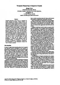
1.1 Structure of this article The goal of this article is threefold: 1) We will use machine-control to introduce the basic reinforcement learning terminology. 2) We will then compare the different neuronal models for reward-based TD-learning, which are used in so-called actor-critic architectures of animal control, with each other and with the anatomy and physiology of the basal ganglia. Here we will strongly focus on the biophysics of dopaminergic synapses and try to provide a summary of the most essential synaptic mechanisms which so far have been identified. (3) Finally we will compare reward-based learning mechanisms (e.g. TD-learning) with correlation-based Hebbian learning trying to relate them to the basic mechanisms of long term potentiation (LTP) and long term depression (LTD) as found in spike-timing dependent plasticity (STDP). Fig. 1 shows the layout of the remainder of this article. This figure depicts the most important links between the different subfields and algorithms, the most influential ones shown in red. The 4

article will proceed from left (machine-learning) to right (synaptic plasticity). The flow in the different chapters (direction of the arrows) is always from top to bottom, except for all “green” components, which are concerned with biophysical aspects. Here we proceed upwards. For specific reviews on the three different fields we refer the reader to: reinforcement learning (Kaelbling et al., 1996; Sutton and Barto, 1998); animal conditioning (Sutton and Barto, 1990; Balkenius and Moren, 1998); the dopamine reward system of the brain (Schultz, 1998; Schultz and Dickinson, 2000; Schultz, 2002); data and models of synaptic plasticity (Martinez and Derrick, 1996; Malenka and Nicoll, 1999; Benett, 2000; Bi and Poo, 2001; van Hemmen, 2001; Bi, 2002).

2 The basic concepts of reinforcement learning It is fair to say that currently almost all methods for predictive control in robots rely on reinforcement learning (RL) and strong indications exist in the literature this type of learning plays a central role in animals, too. A major thread which is followed throughout this article concerns the distinction between reward-based versus correlation-based learning methods, or between evaluative versus non-evaluative feedback (Fig. 7,9). Reinforcement learning (RL) at least in its original formulation is strictly reward-based. Hence an early conclusion would be that animals rely heavily on reward-based learning. Synaptic plasticity on the other hand is correlation-based (Hebbian). How can this apparent conflict be resolved? How can reward-based mechanisms be Machine Learning

Classical Conditioning

Anticipatory Control of Actions and Prediction of Values

Synaptic Plasticity Correlation of Signals

REINFORCEMENT LEARNING

UN-SUPERVISED LEARNING

example based

correlation based

Dynamic Prog. (Bellman Eq.)

d-Rule supervised L.

Hebb-Rule

= Rescorla/ Wagner

LTP (LTD=anti)

= Eligibility Traces TD(l) often l=0

TD(1)

Differential Hebb-Rule (”slow”)

TD(0)

= Neur.TD-formalism

Monte Carlo Control

STDP-Models Neur.TD-Models Actor/Critic

ISO-Learning

(“Critic”)

SARSA

ISO-Control

STDP

Biophys. of Syn. Plasticity

Correlation based Control (non-evaluative)

biophysical & network

ISO-Model of STDP

technical & Basal Gangl.

Q-Learning

Differential Hebb-Rule (”fast”)

Dopamine

Glutamate

Neuronal Reward Systems (Basal Ganglia) NON-EVALUATIVE FEEDBACK (Correlations)

EVALUATIVE FEEDBACK (Rewards)

Figure 1: Cross links between the different fields (see text). Small equal signs denote that these algorithms produce identical results after convergence.

5

re-formulated such that they can be captured by correlation-based learning rules? And, what are the problems when trying to do this? These are the questions which we would like to address in the remainder of this article. For those who might want to skip all the rest of this article lets try to summarize its conclusions in a single sentence here: The central message of this article will be that reward-based and correlation-based methods are very similar if not identical in the open-loop condition, where the actions of the learner will not influence the learning, while they are clearly different in the closed loop condition, hence during the normally existing behavioral feedback. The algorithms for reinforcement learning are treated to a great extent in the literature (Sutton and Barto, 1998) and shall not be described here, but we must describe the basic assumptions of RL, to be able to compare it to animal learning. To this end we will only discuss systems with a finite number of discrete states, commonly known as finite Markov Decision Problems (MDP1 ). We assume that an RL-agent is able to visit these states and that these states will convey information about the decision problem. RL further assumes that in visiting a state, a numerical reward will be collected, where negative numbers may represent punishments. Each state has a changeable value attached to it. From every state there are subsequent states that can be reached by means of actions. The value of a given state is basically defined by the averaged future reward which can be accumulated by starting actions from this particular state. Here we could look at all or just at some of the followup actions which are possible in starting from the given state. The different algorithms for RL take different approaches towards reward-averaging which, however shall not be discussed here. Actions will follow a policy, which can also change. The goal of RL is to maximize the expected cumulative reward (the “return”) by subsequently visiting a subset of states in the MDP. This, for example, can be done by assuming a given (unchangable) policy. Often, however, a sub-goal of RL is to try to achieve this in an optimal way by finding the best action policy to travel through state space. In this context, RL methods are mainly employed to address two related problems: the Prediction- and the Control Problem. 1. Prediction only: RL is used to learn the value function for the policy followed. At the end of learning this value function describes for every visited state how much future reward we can expect when performing actions starting at this state. 2. Control: By means of RL, we wish to find that particular set of policies which maximizes the reward when travelling through state space. This way we have at the end obtained an optimal policy which allows for action planning and optimal control. 1

Thus, RL also assumes that such systems “follow the Markov property”. Essentially this means that it is unimportant along which path a certain state has been reached. Once there, the state itself contains all relevant information for future calculations. Many times the Markow Property cannot be guaranteed in real world decision problem which poses practical problems when wanting to employ RL-methods. Also, we note that conventional RL needs to be augmented by additional mechanisms, if one wants to employ it to more complex, for example time and space-continuous, systems. These aspects shall not be discussed here, but see Reynolds (2002); Santos and Touzet (1999a,b).

6

Several algorithms have beed designed to calculate or approximate value functions and/or to find optimal action policies. Most notably: Dynamic Programming (Bellman, 1957), Monte Carlo Prediction and Control, TD-learning (Sutton, 1988), SARSA (Rummery, 1995; Sutton, 1996) and Q-learning (Watkins, 1989; Watkins and Dayan, 1992). They are reviewed in Sutton and Barto (1998). Most of the above named algorithms for RL rely on the method of “temporal differences” (TD-methods). The formalism of this method is described in the Appendix and its “neuronal” version later in the main text. Using the method of temporal differences, the rewards, which determine learning, enter the formalism in an additive way (Eq. 23). Thus, TD-methods are in the first instance strictly non-correlative as opposed to Hebb-rules, where a multiplicative correlation of pre- and post-synaptic activity drives the learning. Thus, at first it seems hard to introduce a correlative relation in RL to make it compatible with synaptic plasticity, hence with Hebbian learning. Two observations can be made to mitigate this situation. First, we note that the backward TD(λ) method (see Appendix) contains so called eligibility traces x which enter the algorithm in a multiplicative way (Eq. 31) and can, thus, be used to define a correlation-based process. The concept of such traces shall be explained in a more neuronal context to a great detail in section 3. Here it suffices to say that this way TD learning becomes formally related to Hebbian learning. There is, however, a more interesting and but also more problematic way to introduce a correlation-based process which is in particular of relevance for biological or bio-mimentic agents: One could try to define the rewards (or punishments) by means of signals derived from sensor inputs. Naively: Pain is a punishment, while Pleasure is a reward. Thus, rewards can be correlated to sensor events. This seems to be a simple and obvious way to introduce a correlationbased process mainly used in so-called Actor-Critic models of machine or animal control, which shall be introduced later (section 4.1). Actor-Critic Architectures are closed-loop control structures, where the actions of the agent (the animal) will influence its own (sensor) inputs. Thus, before we can discuss those, we must first describe the different algorithms in their open loop versions.

3 Neuronal architectures for prediction and control - open loop condition The goal of the next sections will be to transfer the above discussed concepts of RL, for example TD-learning, to neural networks related to different brain structures. At the same time we would like to discuss other algorithms which are less directly related to the RL formalism.

3.1

Relating RL to classical conditioning

Classical conditioning represents in its simplest form a learning paradigm where the pairing of two subsequent stimuli is learned such that the presentation of the first stimulus is taken as a predictor of the second one. In the descriptions above we have indeed discussed the prediction

7

problem but we have only treated the (action driven) transition between states. Only a vague indication has been given so far about how to use temporally correlated signals for learning. Thus, the goal of this section is to show of how to augment the above discussed aspects such that we can utilize correlations for learning. This way we will see that reinforcement learning and (differential) Hebbian learning are related to each other. 3.1.1

Early neural differential Hebbian architectures

In the traditional example of Pavlov’s dog (Pavlov, 1927), we have the unconditioned stimulus (US) “food” which is preceded by the conditioned stimulus (CS) “bell”. The CS predicts the US and after learning the dog starts salivating already in response to the CS. Note, this represents an open-loop paradigm: The action of salivating will not influence the presentation of the stimuli. This is different from instrumental conditioning which represents a closed loop paradigm, to be discussed later in the context of Actor-Critic Architectures. A model of classical conditioning should, thus, produce an output which - before learning responds to the US only, while after learning the output should occur earlier already in response to the CS. Furthermore, we note that US and CS are temporally correlated. To capture this we need a correlative property in reinforcement learning which in its machine-learning formalism (see Appendix) is not immediately visible, because machine-learning entirely relies on the transition between states by means of actions and correlations do not play any role. This, however, can be achieved by using eligibility traces2 . To this end, we need to restructure the formalism in a neuronal way, where stimuli converge via synapses at a neuron. These architectures are in the context of classical conditioning generally called stimulus substitution architectures, because the first, earlier stimulus after learning substitutes in effect the second, later stimulus. The goal is to generate an output signal at this neuron that will at the end of learning directly respond to the CS. This way the output can be used as a predictor signal for other processes, e.g. for control. This should be achieved by strengthening the synapse which transmits the CS during learning. Fig. 2 shows such a structure at the beginning of learning. Note that this model level is still quite far removed from the biophysical models of synaptic plasticity which shall be discussed later. The US converges with a strong, driving synapse ω0 at the neuron. To keep things consistent with the descriptions above one could call the US “reward”. The CS precedes the US and converges with an initially weak synapse ω1 . However, the CS elicits a decaying trace (e-trace) at its own synapse. This, biophysically unspecified, trace is meant to capture the idea that the CS-synapse remains eligible for modification for some time after the CS has ended. We can now correlate the output V , which at the beginning of learning mirrors the US, with this eligibility trace and use the result of this correlation depicted by ∆ω1 to change the weight of the CS-synapse. This idea has first been formalized by Sutton and Barto (1981) in their classical 2

Historically eligibility traces had first been developed in the context of classical conditioning models (Hull, 1939, 1943; Klopf, 1972, 1982) and were only later introduced in the context of machine-learning Sutton (1988); Singh and Sutton (1996). Our review puts its emphasis on the structural and functional similarities of the different algorithms, therefore we do not follow the historical route.

8

X1

CS

x

e-trace

Dw1 + w1

v(t) X0

w0 = 1

US (reward)

Figure 2: Simple correlative temporal learning mechanism applying an eligibility trace (e-trace) at input x1 (CS) to assure signal overlap at the moment when x0 (US) occurs; ⊗ denotes the correlation. modeling study3 : ω1 (t + 1) = ω1 (t) + γ[v(t) − v(t)]x(t),

(1)

where they have introduced two eligibility traces, x(t) at the input and v(t) at the output, given by: x(t + 1) = αx(t) + x(t) v(t + 1) = βv(t) + (1 − β) v(t),

(2) (3)

with control parameters α and β. Mainly they discuss the case of β = 0 where v(t) = v(t − 1), which turns their rule into: ω1 (t + 1) = ω1 (t) + γ[v(t) − v(t − 1)]x(t),

(4)

Before learning this neuron will only respond to the US, while after learning it will respond to the CS as well. In a later review, Sutton and Barto (1990) discuss that their older model is faced with several problems. For example, for short or negative inter-stimulus intervals (ISIs) between CS and US, the model predicts strong inhibitory conditioning (see Fig. 8 in Sutton and Barto 1990). Some reports exist that indeed show weak inhibitory conditioning but mostly weak excitatory conditioning seems to be found in these cases as well4 (Prokasy et al., 1962; Mackintosh, 1974, 1983; Gormezano et al., 1983). 3 Here we should briefly mention that we have deliberately not discussed some of the older work, like the Rescorla-Wagner rule (Rescorla and Wagner 1972, Fig. 1) or the δ-rule of Widrow and Hopf (Widrow and Hoff, 1960), which is at the root node of all these algorithms. Indeed analytical proofs exist that the results obtained with the δ-rule are identical to those obtained with the Rescorla Wagner rule (Sutton and Barto 1981, pg. 151) and the TD(1) algorithm (Sutton 1988 pg.14–15), denoted by the small equal signs in Fig. 1. 4 More problems are discussed in Sutton and Barto (1990) for example with respect to the so-called “delayconditioning” paradigm which can be solved by some specific modifications of the Sutton and Barto (1981) model. We refer the reader to Sutton and Barto (1990) for these specific issues.

9

C A

XN

hN

X1

h1

xN

0.20

w1

0.16 0.12

x1

wN

w1 X0

h0

x0

0.08

V

S w0

0.04 0

Dw

B

0 5e4 15e4

25e4 35e4 45e4 t [steps]

D 0.00050 wi -0.0005

T

-0.001 -0.0015

Topt

-0.002 -0.0025 0

30

60

90 120 t [s]

150

Figure 3: Isotropic sequence order learning. A) Structure of the algorithm for N + 1 inputs. For notations see text. A central property of ISO-learning is that all weights can change. B) Weight change curve calculated analytically for two inputs with identical resonator characteristics (h). The optimal temporal difference for learning is denoted as Topt . C) Linear development of ω1 for two active inputs (x0 , x1 ). At time-step 40000 input x0 is switched off and, as a consequence of the orthogonality property of ISO-learning, ω1 stops to grow. D) Development of 10 weights ω1i , i = 0 . . . 9 in a robot experiment (Porr and W¨org¨otter, 2003a). All weights are driven by input x1 but are connected to different resonators hi1 , which create a serial compound representation of x1 (see Fig. 10 A). The robot’s task was obstacle avoidance. At around t = 150 s, it has successfully mastered it, and the input x0 , which corresponds to a touch sensor is not anymore triggered. As a consequence we observe that the weights ω1i stop to change (compare to C). 3.1.2

Isotropic Sequence Order learning

Some of the problems of the Sutton and Barto (1981) model come from the fact that input lines are not treated identical, which leads to an asymmetrical behavior of this model. In a more recent approach we have achieved this by employing a different differential Hebbian learning rule onto all synaptic weights (Porr and W¨org¨otter, 2002, 2003a,b). The main distinguishing features of isotropic sequence order learning (ISO-learning) are: 1) All input lines are treated equal. Thus, there is no a priori built in distinction between CS and US and all lines learn. 2) Eligibility traces are created by band-pass filtering the inputs 3) Learning is purely correlation-based and synapses can grow or shrink depending on the temporal sequence of their inputs. 4) Inputs can take any form of being analogue or pulse-coded. As a consequence this approach is linear. Fig. 3 A shows the structure of the algorithm The system consists of N + 1 linear filters h

10

receiving inputs x and producing outputs x¯: x¯i = xi ∗ hi

(5)

where the asterisk denotes a convolution. The transfer functions h shall be those of bandpass filters. They are specified by: 1 h(t) = eat sin(bt) (6) b with: q a := Re(p) = −πf /Q, b := Im(p) = (2πf )2 − a2 (7) f is the frequency of the oscillation and Q the damping characteristic. To get an idea what these filter do, lets consider pulse-inputs. In this case the filtered signals will consist of damped oscillations (Grossberg and Schmajuk, 1989; Grossberg, 1995; Grossberg and Merrill, 1996) which span across some temporal interval until they fade. Thus, band-pass filtering essentially amounts to applying an eligibility trace to all inputs. The filtered signals connect with corresponding weights ω to one output unit v. The output v(t) is given as: v(t) =

N X

ωi x¯i

(8)

i=0

Learning takes place according to a differential Hebbian learning rule: d ωi = µ¯ xi v 0 dt

µ1

(9)

where v 0 is the temporal derivative of v. Note that µ is very small. See Porr and W¨org¨otter (2003a) for a complete description of the ISO-learning algorithm and its properties. First we note that the system is linear and weight-changes can be calculated analytically (Fig. 3 B) as shown in Porr and W¨org¨otter (2003a). Note, if we consider just one input then we find that it is after filtering orthogonal to the derivative of its output. Intuitively this can be understood when looking at two pulse inputs x0 , x1 . In this case both trace-signals x¯0 , x¯1 are damped sine-waves and the derivative of the output is, thus, a sum of damped cosine-waves. Thus, if one input becomes zero, the derivative of the output will be orthogonal to the remaining input. Mathematically it can be shown that this holds for more than two inputs, too (Porr and W¨org¨otter, 2003a). Thus, inputs will not influence their own synapses and learning is strictly hetero-synaptic. As a consequence of this, a very nice feature emerges for pairs of synapses: Weight-change will stop as soon as one input becomes silent (Fig. 3 C). This leads to an automatic self-stabilizing property for the network in control applications (Fig. 3 D, see also section 4.3.1). 3.1.3

The basic neural TD-formalism and its implementation

Most influential in the field of neuronal temporal sequence learning algorithms, however, is currently the TD-formalism. To define it in a neuronal way we replace the “states” from traditional RL with “time-steps”, and assume that rewards can be retrieved at each such time-step. Furthermore, we assume that 11

distant rewards will count less than immediate rewards introducing a discounting factor γ. Then we define the total reward (called the “return”) as the discounted sum of all expected future rewards (similar to the formalism in the Appendix): R(t) = r(t + 1) + γr(t + 2) + γ 2 r(t + 3) + . . . ,

(10)

and this can be rewritten as: R(t) = r(t + 1) + γR(t + 1)

(11)

Now we define a neuron v such that it will function as a “prediction neuron”. To this end, we assume that the output v is able to predict the reward. As a consequence we would hope that R(t + 1) ≈ v(t + 1) and that R(t) ≈ v(t), replacing (compare Eq. 25): v(t) ≈ r(t + 1) + γv(t + 1)

(12)

Since this is only approximately true (until convergence) we can define an error (compare Eq. 29) with: δ(t) = r(t + 1) + γ v(t + 1) − v(t), (13) realizing that this error function contains a derivative-like term: v(t + 1) − v(t), which is shifted one step into the future. This results from the fact that the update of the value of a state requires visiting at least the next following state. In an artificial neural network such as that depicted in Fig. 4 this does not produce problems, but in a rigorous neuronal implementation one should be careful to avoid this acausality, for example applying the appropriate delays or a more realistic eligibility trace (see below). Now we can update the synaptic weights with: ωi ← ωi + α δ(t) xi (t)

(14)

where xi (t) is the eligibility trace associated with stimulus xi . In an older review Sutton and Barto (1990) discuss to what degree this specific TD-model can explain the experimental observations in classical conditioning and they show that it surpasses their older approach in many aspects. This shall not be discussed here, though, because we wish to concentrate next on the “neuronal” aspects of TD-learning, its network implementations, its possible neuronal counterparts in the brain, and its synaptic biophysics. The circuit diagram in Fig. 4 shows a simple implementation of the TD-rule in a neuronal model. It is constructed to most closely relate to the basic neuronal TD-formalism introduced above, keeping the number of necessary parameters minimal. The first neuronal models with an architecture similar to Fig. 4 where devised by Montague et al. (1995, 1996). The goal of our implementation is to arrive at an output v which reacts after learning to the onset of the CS denoted as xn and maintains its activity until the reward terminates. Such an ideally rectangular signal is reminiscent of the response of so-called Reward-Expectation neurons, which shall be shown in section 3.3. To achieve this goal we represent the CS internally by a chain of n + 1 delayed pulses xi , with a unit delay τ which is equal to the pulse width. We construct this chain such that the signal x0 coincides with the reward. In some sense the pulse-chain xi represents a 12

A #1 reward, US

Predictive Signals

Start: w0 = 0 w1 = 0

Start: w0 = 1 w1 = 0

#2

X1

x

X0 x

v

~ v’ End: w0 = 1 w1 = 0

~ r d=v’+ reward

End: w0 = 1 w1 = 1

x

Xn

d x

#3

v ~ v’

X1

~ v’

(n-i)t

v(t)

~ r d=v’+

X0

B

C r d

x

d

x

v(t-t)

t t v(t)

~ v’

X1

X1 v(t)

v(t) X0

w0 = 1

X0

w0 = 1

reward

reward

Figure 4: Basic neural implementation of the TD-rule. A) shows the first three learning steps (#1,#2,#3) performed with the circuit drawn in the shaded inset which represents probably the most basic version of a neuronal TD implementation using a serial compound stimulus representation. The symbol v˜0 represents a forward-shifted difference operation: v˜0 (t) = v(t + 1) − v(t). Other symbols are explained in the text. B,C) Same circuit but using x0 as reward signal. C) here the acausal forward shift of the difference operation is avoided by introducing unit delays τ into the learning circuits. This allows calculating the derivative by means of an inhibitory interneuron (black).

special (distributed) kind of eligibility trace; it is often called a serial compound representation (Sutton and Barto, 1990) first used in a neural network architecture by Montague et al. (1996). The pulse protocols #1, #2 and #3 in Fig. 4 show the first three trials for this algorithm starting with all weights at zero. Thus, in the first trial (#1) the output v is zero and a positive prediction error δ occurs together with the reward. The weight change is calculated using Eq. 14 with ∆ωi = δ xi . Thus, in the first trial #1 only the multiplication of x0 with δ will yield a result different from zero and only this weight changes. In the next trial, v reacts together with x0 ; the 13

derivative is shown below already time-shifted by one step forward as demanded above. As a consequence δ moves also forward (Montague et al., 1996) and now the correlation between x1 and δ yields 1. This process continues in trial #3 where we only show a few traces and so on until as the last weight ωn grows. As a result v becomes a rectangle pulse starting at xn and ending at the end of the reward pulse. Essentially we have implemented a backward TD(1) algorithm (see Appendix) this way. It is obvious that the special treatment of the reward as an extra line leading into the learning sub-circuitry is not really necessary. Fig. 4 B shows that the input signal x0 can replace the reward signal when setting ω0 = 1 from the beginning. This shows that reward-based architectures are in some cases equivalent to stimulus-substitution architectures and we are again approaching the original architecture of the old Sutton and Barto (1981) model. Note, that the circuit diagram shown in Fig. 4 A,B cannot be implemented with analogue (“neuronal”) hardware because it contains the forward shift of the derivative term denoted by v˜0 . Fig. 4 C shows how to modify the circuit in order to assure a causal structure. This requires adding the unit delay τ in the learning sub-circuits to all input lines (and the reward, if an extra reward-line exists). As a result the δ signal will appear with the same delay. This modification, however, allows us also to introduce a small circuit for calculating the difference term by means of an inhibitory interneuron. The architecture in Fig. 4 C is presumably the simplest way to implement a TD-rule neuronally without violating causality. B Sutton and Barto,1988

A Sutton & Barto, 1981

C ISO-Learning

TD-learning

E x1 x0

X

v’ w1

X

r

X

S

E v

x1

S

x1

h1

v’

x0

h0

w1 S

wi

S

v’ v

v X

Figure 5: (A,B) Comparison between the two basic models of Sutton and Barto and ISO-learning (C). Inputs=x, Eligibility trace=E, reward=r, resonators=h. The symbol v 0 denotes the difference operation between subsequent output values in (A,B) and the a differentiation in (C). The small amplifier symbol represents a changeable synaptic weight ω.

3.2 Comparing correlation based- and TD-methods Let us first compare the formalism of the old Sutton and Barto (1981) model (Eq. 15): ω1 (t + 1) = ω1 (t) + γ[v(t) − v(t − 1)]x(t),

(15)

with the neuronal TD-procedure given by Eq. 16: ωi ← ωi + α [r(t + 1) + γ v(t + 1) − v(t)] xi (t)

14

(16)

Learning in Sutton and Barto (1981) is correlative like in Hebbian learning but depends on the difference of the output v 0 ≈ v(t) − v(t − 1) (Fig. 5 A, Differential Hebbian Learning5 ). FurtherP more, since v(t) = i ωi xi , i ≥ 0 in Eq. 15, we notice that the “reward” x0 does indeed occur in the stimulus substitution model of Sutton and Barto but not as an independent term like in the reward-based TD-procedure. Reward-based architectures, like TD-learning, allow treating the reward as an independent entity, which arises in addition to the sensor signals x (Fig. 5 B). Thus, a reward signal could also be an intrinsically generated signal in the brain, which is not necessarily, or only indirectly, related to sensor inputs as discussed above. In view of the neuronal response recorded in the basal ganglia this concept has strong appeal. This was one of the reasons why the TD-formalism has been adopted to classical conditioning. How does ISO-learning (Fig. 5 C) compare to these methods? ISO-learning uses different eligibility traces than Sutton and Barto (1981); Sutton (1988) and employs them at all inputpathways. Hence, they will influence learning via the output v (more specifically via v 0 ). In the models of Sutton and Barto (1981) and Sutton (1988) an eligibility trace is only applied at input x1 and influences only the learning circuit, but not the output v. Thus, for more than two P P inputs we find for ISO-learning that v = ωi x¯i while for TD-learning we have v = ωi xi . If we assume, as before, that x0 is identical to the reward signal and by handling the notation concerning the derivatives in a somewhat sloppy way, we can rewrite the weight change in TDlearning (Eq. 16) as: X dωk = (x0 + v 0 )¯ xk = (x0 + ωi x0i )¯ xk (17) dt i>0 and that of ISO-learning: X dωk = v 0 x¯k = ( ωi x¯0i )¯ xk dt i=0

(18)

As opposed to ISO-learning, the derivative in TD-learning is not applied to the reward and the output is an unfiltered (no traces) sum of the weighted inputs. These differences prevent TDlearning from being orthogonal between in- and outputs. 3.2.1

Conditions of convergence

Furthermore, we note that conditions of convergence are different in ISO- as compared to TDlearning. Trivially, weight growth of ω1 stops in both algorithms when x1 = 0. Otherwise weight growth stops in TD-learning when r(t+1)+γ v(t+1)−v(t) = 0; a condition which requires the output to take a certain value (output condition). The orthogonality between input and output in ISO-learning, on the other hand, leads to the situation that dω1 /dt = x¯1 v 0 = 0 if x0 = 0, which is an input condition. It is interesting to discuss how this would affect animal learning in closed loop situations with behavioral feedback. Animals cannot measure their “output”. All they can do is sense the consequences of an action, hence sense the consequences of some produced output (behavior) after it has been transmitted back to the animal via the environment (see Fig. 7). Thus, 5

Other early differential Hebbian models have been devised by Kosco (1986) and Klopf (1986), who employ a derivative at the CS input to account for its possible inner transient representation.

15

immediate output control can only be performed by an external observer, which might however, misjudge the validity of an action leading to bad convergence properties of such an algorithm. Alternatively augmented output control could be performed by the learner after environmental filtering via its input-sensors. This, however, might also go wrong if the filtering is not benign. Thus, there is a clear difference between input and output control as discussed below (section 4).

16

Novelty Response: no prediction, reward occurs

A

After learning: predicted reward occurs

r

no CS

E

Continuous decrease of novelty response during learning

CS

1.0 s

Response Transfer (Population Response)

F

L

r

K

C

After learning: predicted reward does not occur

r

CS

D

B

G

H

I

J

0.5 s

In

Reward Expectation

Tr

Tr Tr

r

Reward Expectation (Population Response)

r

L

r

1.0 s

1.5 s

Figure 6: Neuronal response in the basal ganglia concerned with reward processing. (A) Response of a dopamine neuron in monkey to the presentation of a reward (r, drop of liquid) without preceding CS. (B) Response of the same neuron after learning that the CS will predict the reward. The neuron now responds to the CS but not to the reward anymore. (C) If the expected reward fails to be delivered the neuron will be inhibited [A-C, recompiled from Schultz et al. (1997)]. (D) Reduction of novelty response during learning. From top to bottom the number of trials increases in chunks of 5 equivalent to a growing learning experience [D recompiled from Hollerman and Schultz (1998)]. (E-J) Response transfer to the earliest reward-predicting stimulus [recompiled from Schultz (1998)]. (E) Control situation, presentation of a visual stimulus (light, L) will not lead to a response. (F) Novelty response, situation similar to A. (G) Response to a reward predicting “Trigger (Tr)” stimulus (similar to B, left part of diagram) and (H) failure to respond to a correctly predicted reward (similar to B, right part of diagram). (I) Response to a newly learned “Instruction (In)” stimulus which precedes the trigger. (J) In the same way, no response to the correctly predicted reward. (K) Response of a putamen neuron which gradually increases and maintains its firing after a trigger until the reward is delivered [(K) recompiled from Hollerman et al. (1998)]. (L) Population diagram of 68 striatal neurons that show an expectation of reward type response [(L) recompiled from Suri and Schultz (2001)].

3.3 Neuronal reward systems Before we will try to embed the different algorithms into “behaving systems”, hence into closeloop architectures, we would like to open a bracket and show, why the reward paradigm appears to be so strong in animal learning. So far we are still at the level of artificial neural network implementations of the TD rule and we have only in passing mentioned that a neurophysiological 17

motivation for this exists - the dopaminergic reward system. The computational focus of this review does not allow for an in-depth discussion of this topic, but some of the most important facts should be described to motivate the corresponding modeling approaches discussed in section 4.2 below. Different response types are found in the mammalian brain, which seem to be related to reward processing. We associate a few of them rather directly with the nomenclature of TDlearning noting that this is an oversimplification which is necessary to fit them into the perspective of a theoretician. For more detailed discussions see Schultz (1998); Schultz and Dickinson (2000); Schultz (2002). Most importantly one finds: 1. Prediction-Error Neurons: Dopamine neurons (DA-neurons) in the pars compacta of the substantia nigra and the medially adjoining ventral tegmental area. These neurons seem to essentially capture the properties of the δ-signal in TD learning (Miller et al. 1981; Schultz 1986; Mirenowicz and Schultz 1994; Hollerman and Schultz 1998 for reviews see Schultz 1998; Schultz and Dickinson 2000; Schultz 2002, but see Redgrave et al. 1999). In addition, they respond to novel, salient stimuli that have attentional and possibly rewarding properties. Before learning these neurons respond to an unpredicted reward (Fig 6 A). During learning this response diminishes (Fig 6 D, Ljungberg et al. 1992; Hollerman and Schultz 1998) and the neurons will now increase their firing in response to the rewardpredicting stimulus (Fig 6 B). The more predictable the reward becomes the less strongly the neuron fires when it appears. The δ-signal in TD learning essentially corresponds to δ = reward occurred − reward predicted. Thus, these neurons respond with an inhibitory transient as soon as a predicted reward fails to be delivered (“Omission”, Fig 6 C). Furthermore, these neurons show response transfer properties: When an earlier rewardpredicting stimulus is introduced, the response of the neuron will during learning move forward in time and begin to coincide with the new, earlier stimulus (Fig 6 E-J).

18

2. Reward-Expectation Neurons: In the striatum, orbitofrontal cortex and amygdala6 (Hollerman et al., 1998; Tremblay et al., 1998; Tremblay and Schultz, 1999). They respond with a prolonged maintained discharge following a trigger stimulus until the reward is delivered (Fig 6 K,L). Thereby they are similar to the “neuron” in Fig. 4. Delayed delivery prolongs the response, while earlier delivery shortens it. Early during learning those neurons will always start to fire following the trigger stimulus apparently “naively” expecting a reward in every trial. Only with experience, responses become specific to the actual reward predicting trials. In addition, it has been suggested that these neurons fire mainly as a consequence of the motivational value of the reward and less strongly following its actual physical properties. Hence, in trials where rewards are compared they seem to estimate the relative value of the different rewards with respect to each other instead of reacting to all of them in an absolute manner. 3. Goal-Directed Neurons: In the striatum, the supplementary motor area and the dorsolateral premotor cortex (Kurata and Wise, 1988; Schultz and Dickinson, 2000). These neurons show an enhanced response prior to an internally planned motor action towards external rewards but in absence of a triggering stimulus. Some neurons continue to fire until the reward is retrieved, other stop as soon as or just before the motor action is initiated. Using the terminology from above, one can interpret the first two types of neurons as being concerned with the prediction problem, while the third type seems to be involved in addressing the control problem. These single cell data have more recently been augmented by a substantial number of fMRI studies of the human brain which also support the idea that the ventral striatum and other parts of the brain (e.g. amygdala, nucleus accumbens, orbitofrontal cortex) could be involved in the processing of reward- or expectation-related activity (Schoenbaum et al., 1998; Nobre et al., 1999; Delgado et al., 2000; Elliott et al., 2000; Berns et al., 2001; Breiter et al., 2001; Knutson et al., 2001; O’Doherty et al., 2001, 2002; Pagoni et al., 2002) possibly related to TD-models (O’Doherty et al., 2003). However, the functional connectivity and the action of Dopamine are by far more complex than suggested by the above paragraphs. Dopamine neurons ramify very broadly essentially all over the striatum. As a consequence, ever striatal neuron (Lynd-Balta and Haber, 1994; Groves et al., 1995) and large numbers of neurons in superficial and deep layers of the frontal cortex (Berger et al., 1988; Williams and Goldman-Rakic, 1993) is contacted by each DA-neuron. In addition, the responses of dopaminergic neurons vary to a large degree and only a small number resembles those discussed here. Thus, the above interpretations of how the different neuron types are concerned with prediction and control may be too coarse and the DA-system may also to a large degree carry gating, motivational, novelty, saliency (Zink et al., 2003) or other context dependent signals, too. On the other hand, it has been found that Dopamine deficient mice mutants can easily perform reward learning (Cannon and Palmiter, 2003). Evidence that NMDA7 receptors and not Dopamine (D2) receptors seem to be involved in specific reward 6

These neurons are named according to Schultz and Dickinson (2000), sometimes they are also called “RewardPrediction neurons” (Suri and Schultz, 2001). 7 NMDA=N-methyl-D-aspartate

19

processing (Hauber et al., 2000) points in the same direction. (See also the discussion about the synaptic biophysics of the dopaminergic system in this article, section 5.) The above mentioned fMRI studies also cannot help resolving these issues, because they have shown that a variety of different areas can be involved in reward processing while some of them may be strongly modulated by attentional effects as well influencing learning (Dayan et al., 2000). In addition, the restricted spatio-temporal resolution of fMRI makes it of little help in actually designing neuronal models. This complexity cannot be exhaustively discussed in this article and we refer the reader to the literature (Schultz, 1998; Berridge and Robinson, 1998; Schultz and Dickinson, 2000; Schultz, 2002; Dayan and Balleine, 2002).

A

Disturbances

Set-Point Controller

X0

Control Signals

Controlled System

Feedback

B Context Critic Reinforcement Signal

Disturbances

Actor

Actions

Environment

(Controller)

(Control Signals)

(Controlled System)

X0 Feedback

Figure 7: Actor-Critic architecture (modified from Barto 1995). A) Conventional feedback loop controller, B) Actor-Critic control system, where a Critic influences action selection by means of a reinforcement signal.

20

4 Closed loop architectures 4.1 Evaluative Feedback by means of Actor-Critic architectures The action of animals or robots will normally always influence their sensor inputs. Thus, to be able to address the control problem, the above discussed algorithms will have to be embedded in closed loop structures. To this end so-called Actor-Critic models have been widely employed, which are strongly related to control theory (Witten, 1977; Barto et al., 1983; Sutton, 1984; Barto, 1995). Fig. 7 A shows a conventional feedback control system. A controller provides control signals to a controlled system which is influenced by disturbances. Feedback allows the controller to adjusts it signals. In addition, a set-point is defined. In the equilibrium (without disturbance), the feedback signal X0 will take the negative value of the set-point, which represents the “desired state” of the complete system. In the simplest case (set-point=0), this is zero, too. The set-point can essentially be associated with the control goal of the system, reaching it by means of the feedback could be interpreted in the way that the system has attained homeostasis. Part B of this figure shows how to extend this system into an Actor-Critic architecture. The Critic produces evaluative, reinforcement feedback for the Actor by observing the consequences of its actions. The Critic takes the form of a TD-error which gives an indication if things have gone better or worse than expected with the preceding action. Thus, this TD-error can be used to evaluate the preceding action: If the error is positive the tendency to select this action should be strengthened or else, lessened. Thus, Actor and Critic are adaptive through reinforcement learning. This relates these techniques to advanced feed-forward control and feed-forward compensation techniques. However, the set-point is in this more general context replaced by context information. This indicates that that control goal can now be somewhat softened, which makes these architectures go beyond conventional, advanced model-free feed-forward controllers. Many different ways exist to actually implement Actor-Critic Architectures (see Sutton and Barto (1998) for an example). They have become especially influential when discussion animal control and we note that these specific Actor-Critic architectures (Fig. 7) represent regulation problems to which animal control also belongs (Porr and W¨org¨otter, 2004). Other Actor-Critic architectures can also be designed, but shall not be discussed here. Two aspects are especially important for the discussion later-on: Actor-Critic architectures rely on the return maximization principle, which is common to all reinforcement learning paradigms, trying to maximize the expected return by choosing the best actions. Furthermore they use evaluative feedback from the environment. Hence feedback signals that come from the environment are not value-free, instead they are labeled “reward” (positive) or maybe “punishment” (negative). In sections 7.1 and 7.4 we will discuss that these two assumptions may pose problems when considering autonomous creatures.

4.2 Neuronal Actor-Critic architectures In general, all neuronal models for prediction and control which have been described in the literature so far follow an Actor-Critic architecture (Barto, 1995) and are focused on the interactions between the basal ganglia and the cortex (Houk et al., 1995), sometimes including other brain 21

structures as well). Most of the time the Critic (Predictor) is implemented in these models with great detail while the Actor (Controller) is in the earlier studies only rather generally described and more details are only added in recent models. We will first compare the different models of the Critic and at the end of this section the Actors. 4.2.1

The Critic

Reciprocal architectures The implementation of a TD-critic shown in Fig. 4 C is called a reciprocal architecture, because it assumes a reciprocal connection from the central summation neuron via the neuron which calculates δ back to the synaptic modification circuit of the central summation neuron (see also Fig. 8 B,C). These types of models capture some of the basic properties of the observed neuronal responses. For example, the δ-signal resembles the response of Prediction-Error neurons, showing the properties of response transfer and omission, while the v-signal is to some degree similar to the Reward-Expectation neurons. Cortex (C)

Frontal Cortex

Houk et al.

C Thalamus

VP SNr GPi

idealized reciprocal architecture (Montague, Suri)

B

C

STN +

STN GPe

- DA

E

r

D

S(VS) +

S

- DA

Contreras-Vidal & Schultz

r

F

C (PFC)

(C)

Striatum (S)

STN

S

A

S

Berns & Sejnowski

Brown et al.

C +

r

- DA

S

C

GP +

- DA

DA-System

S

-

+ DA

r

(SNc,VTA,RRA)

excitation

inhibition

unspecified (net excitation)

dopaminergic projection that modifies target weight

Figure 8: Matching TD-learning to the basal ganglia. A) Schematic wiring diagram of the basal ganglia showing its main in- and outputs. VP=ventral pallidum, SNr=substantia nigra pars reticulata, SNc=substantia nigra pars compacta, GPi=globus pallidus pars interna, GPe=globus pallidus pars externa, VTA=ventral tegmental area, RRA=retrorubral area,STN=subthalamic nucleus. B-F) Simplified circuit diagrams redrawn from the approaches of different groups adopting the same structure to make them comparable. Cortex=C, striatum=S, DA=dopamine system, PFC=prefrontal cortex, VS=ventral striatum, GP=globus pallidus, r=reward. B and C represent parallelreciprocal architectures where both input streams to the DA-system arise in parallel from the striatum, which in turn receives DA-signals in a reciprocal way. Accordingly D is a divergent (non-parallel) reciprocal architecture where the input to the DA system originates in the cortex via two separate striato-nigral pathways. The architecture in E is parallel, non-reciprocal and that in F is divergent, non-reciprocal. Dashed lines with bullets denote a dopamine synapse. They end at another synapse which is the one that is modified.

Matching model architectures to the brain Fig. 8 shows a simplified circuit diagram of the basal ganglia together with its most important inputs and outputs. We will now compare the existing models to this diagram. For an in-depth treatment of this topic see Daw (2003).

22

• Parallel reciprocal architectures; Houk’s model: The first attempt to match the abstract architecture of a Critic to the structure of cortex and basal ganglia has been made by Houk et al. (1995) (see Fig. 8 B). So called striosomal modules8 fulfill the functions of the adaptive Critic. The prediction-error (δ-) characteristics (Eq. 13) of the DA-neurons of the Critic are generated by: 1) Equating the reward r with excitatory input from the lateral hypothalamus. 2) Equating the term v(t) with indirect excitation at the DA-neurons which is initiated from striatal striosomes and channelled through the subthalamic nucleus onto the DA neurons. 3) Equating the term v(t − 1) with direct, long-lasting inhibition from striatal striosomes onto the DA-neurons. This principle, depicted in Fig. 8 B, is a variation of diagram 4 C, where we have used an interneuron to create the subtractive term. The long lasting inhibitory component used to calculate the subtractive v(t − 1) term by Houk et al. (1995) sub-serves the same purpose. Is this model supported by anatomy and will it produce the correct neuronal responses? At first this comes down to the central question if a reciprocal architecture is supported by the connectivity between striatum and the DA-system. Many models, like Houk’s, make the even more specific assumption that striosomes contain the main part of the rewardpredicting neurons in the striatum with reciprocal connections (Houk et al., 1995; Brown et al., 1999; Contreras-Vidal and Schultz, 1999). This assumption is supported by the work of Gerfen (Gerfen, 1984, 1985; Gerfen et al., 1987; Gerfen, 1992). These studies have shown in rats that there is a reciprocal connection between the striosomes of the dorsal striatum and a small group of DA-neurons of the SNc and SNr. In other species anatomical evidence also supports the notion that at least weak reciprocal connections between both structures exist (Haber et al., 2000; Joel and Weiner, 2000). There is, however, little support for the notion that this reciprocity is sub-compartmentalized, because it does not seem to be the case that mostly the striosomal neurons would take part in a reciprocal connection pattern (Joel and Weiner, 2000). Rather it seems that such connections can exist for striosomal and matrisomal neurons of the striatum in a similar way. • Comparing Houk’s model to idealized parallel reciprocal architectures: Fig. 8 C shows the idealized reciprocal architecture required to implement a TD-rule by means of interactions between cortex (C) and striatum (S). This architecture assumes a direct excitatory pathway and an indirect inhibitory pathway. In reality the situation, however, is reversed (Bunney et al., 1991; Pucak and Grace, 1994; Haber et al., 2000; Joel and Weiner, 2000) and we observe as a second problem that the direct action of striatal activity onto DA-neurons is inhibitory, excitation only arises indirectly as the consequence of disynaptic disinhibition (ventral striatal inhibition of GABAergic neurons in the ventral pallidum, which projects to most of the DA system, Fig. 8 A). Thus, we would obtain a sign inverted situation with −v(t) and +v(t − 1) which is not in accordance with the TD-rule. 8

Striosomal modules consist of striatal striosomes, subthalamic nucleus, and the DA-neurons of the substantia nigra pars compacta. They are called the limbic striatum.

23

In conclusion, there is no support for implementing a reciprocal Critic architecture relying on striosomal neurons only. However, even when relying on the whole population of striatal neurons (including the matrisomal neurons) we are still faced with the sign-inversion problem (Joel et al., 2002). To avoid this, models must make specific assumptions about the time courses of the involved signals. One possible solution to this problem might lie in the different, sometimes very slow, time courses of the different chemical compounds which are involved in the second messenger chains leading to dopamine-related synaptic modification (Houk et al., 1995). We will discuss this in section 5. From a functional point of view we find that the long lasting inhibitory component used to calculate the subtractive v(t) term in Houk’s approach leads to the situation that this model cannot account for the precise timing of the depression during omission of a predicted reward (see Fig. 6). Other timing problems arise as the consequence of the fact that this model has not implemented any kind of serial compound stimulus representation. This was first done by Montague et al. (1995, 1996) in the context of a reciprocal architecture and in the following in several models by Suri and co-workers (Suri and Schultz, 1998, 1999, 2001; Suri et al., 2001). Suri et al do not make an explicit link to anatomy but seem to imply that they are essentially following the approach of Houk. At a closer look, however, their models are more strongly related to the ideal reciprocal architecture (Fig. 8 C) than to Houk’s model (Fig. 8 B). • Divergent reciprocal architectures: So far we have discussed what we would call “parallel-reciprocal” architectures (see Legend of Fig. 8 B,C). These models assume that two parallel pathways exist from the striatum to the DA-system. An alternative source for these two streams is the limbic prefrontal cortex (PFC). Indeed evidence exists that the PFC projects directly to the DA-system (reviewed in Overton and Clark 1997) and that an additional projection exists to the ventral striatum (Groenewegen et al., 1990; Parent, 1990). Via this pathway delayed inhibition could be provided to the DA-system. This is supported by findings that responses in the ventral striatum show reward expectation activity (Schultz et al., 1992). A model which utilizes such a divergent-reciprocal architecture was devised by Brown et al. (1999) (Fig. 8 D). This model uses a special kind of serial compound stimulus representation by assuming a spectral timing approach (Grossberg and Schmajuk, 1989; Grossberg, 1995; Grossberg and Merrill, 1996) of a set of band-pass filtered pulses (resembling in shape that of an EPSP) with different onset-times which cover the whole inter-stimulus interval between CS and US. In their model these pulses represent the supra-threshold internal Ca2+ concentration. The cortex provides excitatory input to the striosomes which project inhibitorily to the DA-system (Fig. 8 D). At the same time the cortex also projects to the ventral striatum. This signal gets transfered via several stages to the DA-system, where it finally exerts an excitatory action. Cortico-striatal synapses are modified in the striosomes as well as in the ventral striatum. This architecture still fulfills the basic properties of a TD-architecture, the nested, multi-stage computation and the synaptic modification rules used, however, do not anymore provide a direct link to the TD-rule. The model re24

produces most of the known experimental data. This is mainly a virtue of the different timing-properties along both legs of the divergent input pathways to the DA-system. This additional degree of freedom avoids several of the timing-problems that have been found in the older models (see discussion in Brown et al. 1999). • Parallel non-reciprocal architectures: Berns and Sejnowski (1998) have devised a parallel non-reciprocal architecture (Fig. 8 E), which in essence resembles the model of Houk et al. (D), but implements several pathways more accurately following the known anatomical structures than any of the other models. This architecture is called non-reciprocal because the weight-modification does not take place in the striatum. In the model of Berns and Sejnowski (1998) weights of the STN→GP connection as well as those of the striato-nigral connection (S→DA) are modified, for which there is currently no direct evidence. The learning rule used is a three-factor Hebbian learning rule. Two factors come from the pre and postsynaptic activity of the concerned connection, the third is a so-called “error-term” e, calculated from the difference between the activity of the GP→DA and the S→DA connection. This error term is used as the reinforcement signal. Thus, this model does not use any primary reinforcement (reward r) and cortical input is also not explicitly mentioned. • Divergent non-reciprocal architectures: The model of Contreras-Vidal and Schultz (1999) (Fig. 8 F) most strongly deviates from the traditional TD-rule. Like in Berns and Sejnowski (1998) it assumes that the striatonigral and not the cortico-striatal synapses are modified by means of the DA-activity. In general, their model focuses on the action of the prefrontal cortex which provides indirect input to the striosomes and from there on to the DA-system. Thus, this model represents a divergent non-reciprocal architecture. The model is fairly opaque and it seems as if this input line will lead to net excitation at the DA-system, which is opposite to the assumption of the other models. Accordingly the second pathway from the prefrontal cortex to the DA-system acts inhibitorily in their scheme (divergent architecture). In addition, they have implemented an adaptive resonance network (ART-2, Carpenter and Grossberg 1987) and use this to model an attentional and orienting subsystem. • Problems with serial compound representations: All of the more recent models use some kind of serial compound stimulus representation to cover the long temporal intervals between the stimuli. The problem of a straight-forward serial compound representation, like the one used in Fig. 4, is that it predicts a gradual shift of the δ-signal forward in time during learning (see steps #1-#3 in Fig. 4, Schultz et al. 1997). This, however is in general not observed in real recordings where the response of the DA-neurons remains in place and gradually diminishes during learning (Fig. 6 D), while the response to the predictive stimulus increases. Furthermore the model in Fig. 4 will also not produce novelty responses to new and salient stimuli which are very often observed in DA-neurons.

25

Accordingly, more recent models where designed solving these problems by means of a more elaborate serial compound stimulus representation. For example, Suri and Schultz (1998, 1999) use a representation where only one delay of 100 ms is used between the first and all other xi , but where all xi , i > 1 are stretched in time with increasing durations and decreasing amplitude. With this architecture they were able to more accurately reproduce the properties of real DA-neurons (Prediction-Error neurons), including novelty responses and avoiding the forward shift of the δ-signal. In this study, they found that only the one specific weight grows which represented the temporal interval between prediction and reward. As a consequence these models can only learn a single inter-stimulus interval correctly. When using other ISIs the model will produce incorrect responses. In their later models Suri and Schultz (2001) and Suri et al. (2001) return more closely to the architecture in Fig. 4 C. In addition to the serial compound representation of the stimulus, they also employ an analogue eligibility trace at every xi , which according to the authors speeds up learning and also leads to the specific shapes of the output responses. They do not show responses of Prediction-Error DA-neurons (δ-signals) during learning, and the complexity of this model is such that it is not immediately evident if it will again produce some kind of forward shift of the δ-signal. One study Suri and Schultz (2001) focuses on the responses of Reward-Expectation neurons in the putamen and the orbitofrontal cortex. The other study implements a so called “extended TD-model” which not only gets external stimulus input but is also internally driven by thalamic activity and by actionrelated signals. Thus, Suri et al. (2001) make serious attempts to implement an Actor. This aspect will be discussed in the next section. There is evidence that neurons in the striatum produce varying response latencies and durations (Schultz, 1998; Schultz and Dickinson, 2000; Schultz, 2002) which could support the idea of a serial compound representation. Furthermore, the different models discussed so far can indeed reproduce a wealth of physiological findings. Still, the valid parameter ranges of the existing models appear rather narrow and the models have to be specifically tuned to reproduce the different response properties of the neurons. In addition, the wiring pattern for the serial compound representation has also to be rather specifically set up and the unknown delay between CS and US requires a large number of neurons in the serial compound representation of xi . Criticizing the Critic In general one finds that there are currently only a few shared principles found in the different models. This concerns structure, where sometimes strongly differing anatomical assumptions are found between the models, as well as function, where different learning rules are used. Parallel reciprocal architectures (Fig. 8 B,C,D), which can be used to implement a neuronal version of the TD-rule, are possibly supported by the connectivity of the basal ganglia. The assumption that such reciprocal connections are restricted to striosomes (which are used for the Critic) does not seem to be valid, though. Idealized reciprocal architectures (Fig. 8 C) which are essentially used in the models of Montague and Suri are not directly supported by anatomy because of the “sign inversion problem” discussed above. From a functional point of view, accurate reproduction of the experimental data requires a fairly complex serial compound 26

representation of the stimulus. This assumption may prove to be too inflexible, too. Divergent architectures (Fig. 8 D,F) and non-reciprocal architectures (Fig. 8 E,F) are not necessarily related to the TD-rule anymore. Especially the divergent architectures offer additional degrees of freedom in adjusting the timing along the different input lines to the DA-system. A serial compound representation is also needed in these models and the question arises if the spectral timing approach of Brown et al. (1999) would be more flexible than the more conventional setup used in the other models. 4.2.2

The Actor

In general, less attention has been payed so far to the implementation of the Actor. This may have to do with the fact that there are only few single-cell recordings available which could be matched to the activity of Actor-cells (Goal-Direction neurons, see section 3.3), as opposed to the Critic, where a wealth of data exist. The performance of the Actor is, thus, judged by observing the obtained actions (“behavior”). The study of Houk et al. (1995) was also the first to suggest of how to design an Actor. The matrix modules9 integrate the information from the striosomal modules (see above) and from cortical inputs in order to create output to the frontal cortex relayed through the thalamus. In contrast to the detailed discussion of the critic, Houk et al. (1995) only provide a rather general scheme of the implementation of the actor. According to their model, matrix modules generate signals that command actions or represent plans that organize other systems to generate the actual commands. Montague and colleagues (Montague et al., 1995, 1996) implement decision units as the Actor in their models. This is not meant to be related to basal ganglia anatomy, rather it represents an abstract binary decision network. The TD-error δ is used to influence the decision probability and to adjust the weights at the decision units appropriately during learning. This architecture allows only for binary decisions. In their 1999 model Suri and Schultz also model a control task with an Actor-Critic architecture. In this model the actor consists of one layer of neurons, each of which represents a certain action. It learned stimulus-action pairs based on the prediction error signal provided by the Critic. A winner-take-all rule, implemented by means of lateral inhibition between the units, assured that only one action was selected at a given time. In combination with the more sophisticated Critic (discussed above) this still rather simple Actor-model was able to solve several relatively complex behavioral tasks. All these Actor-models were still rather simplistic. In a recent model, Suri et al. (2001), however, made serious attempts to implement a more detailed Actor, trying to match it to anatomy as well. Like in Houk et al. (1995), the Actor uses striatal matrisomes. These provide direct inhibition to the GPi/SNr complex (compare Fig. 8 A) and indirect excitation via the GPe and the STN. The GPi/SNr complex projects inhibitorily to the thalamus and from there on excitatorily to the cortex which elicits the actions. The DA-system provides input to the matrisomal 9

Matrix modules consist of the striatal matrix, subthalamic nucleus, globus pallidus, thalamus, and frontal cortex. They are called sensorimotor striatum.

27

neurons of the striatum. Its exerts an effect on the membrane potential of these cells but also on the weight of the cortico-striatal synapses ω essentially with ∆ω = DA × P re × P ost, comprising a three-factor learning rule, which relies on the activity of the DA-system (DA) as well as the pre- and postsynaptic activity at the striatum cell (Miller et al., 1981; Schultz, 1998). The membrane activity of these cells follows the physiological observation that they can be in a depolarized “up-” and a hyperpolarized “down”-state. We defer the reader to section 5 for a more detailed description of these states. Here it seems that this property can improve reaction times as well as learning properties as compared to a model version without such membrane states. As in their older model, Actor-neurons represent single actions each and actions are selected again by a winner-takes-all mechanisms such that the winning inhibition will disinhibit the thalamus. As a consequence the number of possible actions is limited to the number of Actor neurons. The use of internal signals in the extended TD-model of the Critic in the model of Suri et al. (2001) leads to the situation that this model can now also perform some kind of planning. Planning refers to the behavioral strategy that an action can be selected without primary reinforcement, just as the consequence of having memorized previously experienced situation-action pairs. For example; if a reward has always occurred at the right side in a T-maze, the animal will after learning turn right without any external stimulation. Suri et al. (2001) achieve this by means of internal signals which enter the extended TD-model and from there on the Actor-neurons. One could say that these internal signals form an internal, explicit representation of a chain of events which can be utilized for learning and acting. The performance of this model is rich and it reproduces many existing data sets. However, its architecture is fairly advanced and as a consequence it contains many free parameters, few of which have direct physiological support. The assumption that striosomes form part of the Critic while matrisomes belong to the Actor is not supported by the anatomy of the basal ganglia, as discussed above. Therefore it is questionable to employ two different learning rules (TD-rule versus three-factor rule) at these two sets of neurons. From a functional point of view up- and down-membrane states are also found across all medium spiny striatal neurons (for a review see Nicola et al. 2000) and not only in the matrix neurons. Criticizing the Actor From a more conceptional point of view two aspects may be problematic in the currently existing actor models. 1. The number of possible actions is matched to the number of actor neurons. Thus, these neurons represent some kind of “grandmother cell” concept, where only a rather limited number of discrete decisions is possible. This may work in restricted-choice lab situations. The complexity of real-world situations, however, requires a different type of actionnetwork. 2. In general, the basal ganglia include many indirect pathways, which often amount to disinhibition. Disinhibition, however, normally acts permissive or facilatory and cannot directly be equated with excitation. Specific motor commands, on the other hand, require the concerted action of many specific and sometimes temporally rather fine tuned excitations. We believe that the release of inhibition at the thalamus performed by the Actor pathway in 28

for example - the model of Suri et al. (2001) can at best act gating on such motor actions. Thus, action selection by means of such a gating process seems to be too crude a model for animal (motor) control. Disturbances Set-Point Controller Actor&Critic

Control Signals

Action= f(X0 o X1)

X1

Controlled System

X0

early late

Feedback

Figure 9: Correlation-based control architecture, where the control signal is derived from the correlations between two temporally related input signals.

4.3 Non-evaluative correlation-based control Above we have stated that Actor-Critic architectures follow the return maximization principle by means of evaluative feedback from the environment. Fig. 9 suggest a schematic architecture which accommodates a different approach: 1) non-evaluative feedback and 2) disturbance minimization. This architecture utilizes the basic feedback loop controller from Fig. 7 A, but it assumes that the environment will, in a temporal sequence learning situation, provide temporally correlated signals about upcoming events like those mentioned in the introduction (e.g., smell predicts taste, etc.). This architecture follows the learning goal: Learn to keep the later signal (x0 ), whatever it is, minimal by employing the earlier signal (x1 ) to elicit an appropriate action. In conventional actor-critic architectures, the critic provides an evaluation of the action (e.g. “good” or “bad”) and this evaluation influences future action selections. Such evaluations are, however, always subjective. In correlation-based control the situation is fundamentally different: Here the system relies on the objective difference between “early” and “late”, which arises from the structure of the input signals. Evaluations do not take place at this point. Instead the “re-”action of the feedback control loop in response to x0 , be it an attraction or a repulsion reaction, will be shifted forward in time to occur earlier now in response to x1 . Thus, in this system, evaluations do not take place during learning instead they are implicitly built into the (sign of the) reaction behavior of the inner x0 -loop: repulsion or attraction. As a consequence, Critic and Actor are not necessarily separate entities anymore and can be merged into the same architectural building block. Furthermore we note that this control strategy does not seek to maximize returns. On a complex decision topology such maxima (or even near maximal regions) may be hard to find by means of RL. Disturbance minimization, on the other hand, offers the advantage that the associated regions will almost always be much bigger promising better convergence properties.

29

A

XN X1

X0

hN

h1

h0

xN x1 x0

B

t=48s

w1 wN

S

d

V

w0 t=0s

Organism

c

C P0

t

t=153s

P1 Environment

D

e t=186s

Figure 10: Applying ISO-learning in a control task. A) This architecture is reminiscent of an Actor-Critic architecture (see Fig. 7 9), but here the system does not use evaluative feedback (“rewards”) from the environment. Instead it relies only on correlations between the inputs. Hence, it is assumed that the “organism” receives temporally correlated inputs, where x1 arrives earlier (e.g.; a signal from a range finder reflected from an obstacle) and x0 arrives later (e.g.; a signal from a touch sensor triggered at the moment of touching the obstacle). P0 , P1 denote environmental transfer functions, D a signal (“disturbance”), which arrives at the inputs: undelayed at x1 and with delay τ at x0 . Other symbols are as in Fig. 3, here we have also implemented a filter bank of 10 filters with different frequencies all driven by the same input x1 , this way creating also something like a serial compound representation. This, however, was done purely to speed up learning and to create smoother output signals. Note that a filter bank approach does not destroy orthogonality and weights will still self-stabilize (Fig. 3 D). After successful learning, the output V will fully compensate the disturbance D at the summation node of the inner loop leading to x0 = 0, which is equivalent to a functional elimination of the inner loop. The system has learned the inverse controller of the inner loop (Porr et al., 2003). B,C) Trajectory of a real robot early (B) and late (C) during learning in an area with three obstacles (boxes). Collisions are denoted by the small circles (forward=solid, backward=dashed). Only forward collision can be used for learning. In such an environment the robot never needed more than 12 forward collisions to learn the task. This way it is as fast as the best RL-algorithms which require sophisticated credit-structuring and temporal assignment mechanisms. (Touzet 1999 also Touzet pers. communication).

4.3.1

ISO-control: merging Critic & Actor

In this section we will describe how ISO-learning can be used to implement correlation-based control introduced in an abstract way in the previous section. The central assumption of ISOcontrol is that any control system should start with a stable negative feedback loop (Fig. 9) for example a reflex-loop. Feedback controllers, however, suffer from a major disadvantage: They will always only react after a disturbance has taken place (inner loop in Fig. 10 A). Thus, the desired state (e.g. x0 = 0, see also Fig. 9) cannot be maintained all the time. Or in other words, disturbances will not yet be minimal when employing feedback control. ISO-control can improve on this if a temporal correlation exist between the primary disturbance and some other earlier occurring signal (denoted by the delay τ between the inner and the outer loop in Fig. 10). The ISO-learning algorithm allows for learning this correlation and, as a result, the primary reflex 30

reaction will be “shifted forward” in time, now occurring earlier; i.e. before the primary reflex would have been triggered. Thus, if learning is successful the primary reflex will be fully avoided and disturbances are now minimal (ideally zero). Note that in the architecture shown in Fig. 10 A Critic and Actor are not anymore separate (compare Fig. 7 B with Fig 9). There is indeed recent experimental evidence that neurons exist where behavior and reward (actor and critic) are more closely linked (Hollerman and Schultz, 1998; Kawagoe et al., 1998; Hassani et al., 2001). This principle has been employed in several real-robot experiments (Fig. 10 B,C) which can be viewed at http://www.cn.stir.ac.uk/predictor. We simulate touch and range-finder signals. Before learning the simulated robot will perform a built-in retraction reaction when touching an obstacle (primary reflex reaction). All weights ωk are initially zero except the weights which belong to the touch sensor inputs, which we set to one. Thus, the output is at this stage just the signal v = x¯0 , where x¯0 is the band-pass filtered touch senor input x¯0 = h0 ∗ x0 . This signal is sent sign-inverted (negative feedback!), but otherwise unaltered, to the motors10 , which leads to a retraction reaction. The range-finders provide the necessary earlier signal because they respond before the touch sensor is triggered. ISO-learning learns this correlation. After learning the P output is v = ωk x¯k , where k ≥ 1, because the touch sensors (x0 ) are not anymore triggered. This signal will now in same way as before, but earlier, lead to a retraction reaction and the primary reflex will be avoided. Interestingly, the principle of disturbance minimization by reflex avoidance can be employed in the same way to learn a food-retrieval task (see Porr and W¨org¨otter 2003b). Here a behavior emerges which looks like reward-retrieval (or return-maximization) but which really follows the disturbance-minimization principle.

5 Biophysics of synaptic plasticity in the striatum The more recent of the above discussed models of the basal ganglia begin to make rather specific assumptions about cellular and sub-cellular mechanisms. This also requires a discussion. The striatum is currently the best understood substrate concerning the interactions between glutamatergic (Glu) and dopaminergic (DA) synapses. Such interactions also take place in many other brain structures, but shall not be discussed here. Furthermore, we will restrict the discussion to facts which at the moment seem to be fairly generally acknowledged. This is meant to facilitate the computational perspective and should allow us to design restricted but at least valid models without too many open degrees of freedom.

5.1 Basic observations Fig 11 gives a summary of the different types of synaptic modifications at corticostriatal glutamatergic synapses targeting a spiny projection neuron in the striatum. Three possible influences can in principle affect the synapse: 1) presynaptic stimulation of the corticostriatal pathway, 2) 10

This description is slightly simplified, because we employ steering and accelerating control, thus two sets of neurons. The correct cross-wiring is described in Porr and W¨org¨otter (2003a). Here of importance is that ISOcontrol essentially works without any signal post-processing or conditioning.

31

Nigrostriatal (”DA”) DA

Corticostriatal (”pre”)

Glu

Medium-sized Spiny Projection Neuron in the Striatum (”post”)

pre

post

DA

Result

1

X

0

0

0

2

0

X

0

0

3

0

0

X

0

4

X

X

0

LTD (dl)

5

X

0

X

0

6

0

X

X

0

7

X

X

X

LTD (DA tonic) LTP (DA phasic)

LTP (dm)

*

Figure 11: Effects of the different activation protocols on the plasticity of cortico-striatal synapses. Small x in the table denotes an active influence. Only paired pre- and postsynaptic activation (row 4), with or without DA activation (row 7) will lead to synaptic plasticity. For further explanations see text. References for the table rows 1: (Calabresi et al., 1992a; Choi and Lovinger, 1997; Calabresi et al., 1999), 2: (Calabresi et al., 1992b; Choi and Lovinger, 1997; Calabresi et al., 1999), 3: (Calabresi et al., 1987, 1992b; Umemiya and Raymond, 1997), 4:(LTD) (Calabresi et al., 1992b; Lovinger et al., 1993; Walsh, 1993; Wickens et al., 1996), 4: (LTP and mixed effects) (Charpier and Deniau, 1997; Charpier et al., 1999; Akopian et al., 2000; Partridge et al., 2000; Spencer and Murphy, 2000), 5: (nucleus accumbens) (Pennartz et al., 1993), 5:(striatum) (Calabresi et al., 1999), 6: (Calabresi et al., 1999), 7: (LTP with M g 2+ removed) (Calabresi et al., 1992c; Walsh and Dunia, 1993), 7: (LTD with normal conditions, i.e., with M g 2+ ) (Calabresi et al., 1992a,b; Tang et al., 2001), 7: (LTP with pulsed DA application) (Wickens et al., 1996). postsynaptic activation of the projection neuron, and 3) activation of the nigrostriatal, dopaminergic pathway. By itself, none of the three influences can affect the Glu-synapse (top part of table, for literature references see figure legend). If, however, presynaptic corticostriatal stimulation is paired with postsynaptic activity early studies have unequivocally reported that LTD occurs at the Glu-synapse. More recently these observations have been augmented by findings showing that LTP mainly occurs in the dorsomedial (dm) part of the striatum, whereas LTD is found in the dorsolateral (dl) part following the gradient of D2-like receptor density (Joyce and Marshall, 1987; Russell et al., 1992). In addition, the expression of LTP or LTD will also depend on the applied stimulation protocol (for review see Reynolds and Wickens 2002). In general, the tendency for LTD seems to be stronger than that for LTP, indicated by the different font sizes in the table. Failing to pair pre- and postsynaptic activation, on the other hand, will neither induce LTP nor LTD, regardless of the activation state of the dopaminergic pathway. The most robust protocol to induce LTP or LTD consists of the stimulation of all three influences. It was found that tonic, long-lasting activation of the DA-pathway will induce LTD (Calabresi et al., 1992a,b; Tang et al., 2001), whereas phasic, pulse-like activation, which leads to a less-strong D1-like receptor desensitization (Memo et al., 1982), will lead to LTP (Wickens et al., 1996). Thus, this has been called a “three-factor” learning rule (Miller et al., 1981; Schultz, 1998). This terminology, however, may be misleading. Dopamine is a potent modulator of synaptic plasticity, but should not 32

enter the equation in a multiplicative way, because the conjoint action of pre- and postsynaptic influences (middle of table, row #4) seems to suggest that two factors already suffice for synaptic modification, and in this case we would ideally set “dopamine=0”. It is, however, currently a matter of debate if the dopamine concentration indeed approaches zero under these experimental conditions, because traces of DA can be detected by HPLC11 following high frequency stimulation of the corticostriatal pathway (Calabresi et al., 1995). Thus, it is still conceivable that under physiological conditions the lack of a DA-signal would prevent LTP or LTD altogether, because chronic near total depletion of DA prevents LTD (Calabresi et al., 1992a) and LTP (Centonze et al., 1999) (chronic denervation protocols). As a consequence, the validity of the three-factor rule can still not be conclusively ruled out.

5.2 Intra-cellular processes Fig. 12 shows a summary of the intracellular actions which take place at DA- and Glu-synapses as far as they are understood today. The diagram is to some degree simplified and more detailed accounts can be found in Greengard et al. (1999); Centonze et al. (2001). Both, LTP and LTD, are introduced in the striatum by repetitive stimulation of the corticostriatal fibers and this event produces massive release of both, glutamate and dopamine, in the striatum dopamine acts mainly via two receptor sub-types (D1-like, and D2-like, Sibley and Monsma 1992), and we consider here the action of glutamate onto AMPA12 and NMDA13 receptors only. The more modulatory action of metabotropic glutamate receptors shall not be discussed. Synaptic strength, measured for example by the size and slope of EPSPs, can partly be associated to the number and phosphorilated AMPA and NMDA receptors (p-AMPA and p-NMDA) which are integrated into the membrane, while dephosphorilated receptors are not active. In general, one observes that LTP only occurs when NMDA channels are active (Calabresi et al., 1996; Yamamoto et al., 1999; Partridge et al., 2000), which in experimental in vitro conditions can be achieved by removing Mg2+ from the medium (Calabresi et al., 1992c, 1996; Centonze et al., 1999). In vivo, this would require a depolarized state of the neuron, where the Mg2+ -block at the NMDA-channels is lessened or removed. LTD on the other hand is independent of the NMDA-channels (Calabresi et al., 1996; Yamamoto et al., 1999; Partridge et al., 2000) and can, thus, also take place in vivo during less depolarized membrane states. Basically we distinguish three pathways which can lead to the modification of the synaptic strength of the Glu-synapse (Fig. 12 A). 1. Glu-NMDA-Ca2+ -CaMKII Pathway (right side of the diagram): This pathway is the traditional pathway involved in the generation of LTP. During elevated Calcium levels the increased activity of CaMKII leads to an increase in the phosphorilated receptors at the membrane. A counter-action arises, however from PP-2B which gets stimulated by Ca2+ and leads to a dephosphorilation of DARPP3214 (King et al., 1984; Nishi et al., 1997). This 11

HPLC=High pressure liquid chromatography AMPA=alpha-amino-3-hydroxy-5-methyl-4-propionate 13 NMDA=N-methyl-D-aspartate 14 dopamine and cyclic adenosine 3’-5’-monophosphate-regulated phosphoprotein, 32kDa 12

33

A

DA

Receptor types Dopamine

AMPA

DA

Ca

NMDA

NO

DA

Glutamate

NMDA

AMPA

P

cGMP

Ca

2+

PKG

PP-1

Ca

5) (T7

2+

L-Ca

CaM

(T34)

cAMP 2+

D1-like D2-like

Glu

CaMKII

p-DARPP32 T75

PKA

PP-2B

T34

DARPP32

B

Glu

NMDA

AMPA

P

DA

Ca

2+

CaMKII

Ca

PP-1

(T34)

cAMP

Ca

CaM

p-DARPP32

2+

2+

PP-2B PKA

T34

DARPP32

DA

C Glu DA

NO AMPA

P

DA

Ca

NMDA Ca

2+

PP-1

cGMP

2+

CaM CaMKII

cAMP

p-DARPP32 PKG ) (T75

PP-2B

T75

PKA

DARPP32

Figure 12: Biophysics of striatal synapses (see text). acts dephosphorilating onto the receptors along the second pathway discussed next. Note, the complete cascade involved in the first pathway is more complex than drawn here, but see section 6.1 for a more detailed discussion of the literature. 2. DA-D1-PKA-pDARPP32 Pathway (outer left part of the diagram): The action of dopamine onto D1-like receptors leads to an elevated level of cyclic AMP (cAMP) and increased PKA stimulation (Stoof and Kebabian, 1981). PKA can directly act phosphorilating on AMPA channels (Roche et al., 1996; Tingley et al., 1997). At the same time PKA shifts the equilibrium of DARPP32 towards its active phosphorilated form (p-DARPP32) by phosphorilating its Threonine-34 residue (T34 in diagram: DA induced Nishi et al. (1997), adenosine induced Svenningsson et al. 1998) which inhibits the action of PP-1 (protein 34

phosphatase-1, Hemmings et al. 1984). The protein PP-1 normally acts dephosphorilating at Glu-receptors. Thus, for this pathway we find an inhibition (by p-DARPP32) of dephosphorilation (by PP-1). In a side path, PKA also helps phosphorilating L-type Ca2+ channels (Surmeier et al., 1995) which adds to the Calcium pool. 3. DA/NO-D2-PKG-pDARPP32 Pathway (inner left part of the diagram): The action of dopamine onto D2-like receptors seems less well understood. Recent observations from Calabresi et al. (2000) suggest that there is at least a two-fold action possible. It seems that dopamine can directly act on the D2-like receptors which leads to an inhibition of PKA (Centonze et al., 2001). However, at the same time there exists an indirect pathway via NO-syntase positive interneurons (Morris et al., 1997). At these neurons, dopamine acts on D1-like receptors15 which leads to the release of NO at their terminals. NO enhances the level of cGMP (Altar et al., 1990) and stimulates PKG. PKG increases the level of phosphorilated DARPP32, this time, however, phosphorilating Thr34 and Thr75 (T75 in diagram (Calabresi et al., 2000)). This type of phosphorilated DARPP32 acts inhibiting onto PKA (Bibb et al., 1999) but cannot efficiently inhibit PP-1. As a consequence, dephosphorilation can take place more easily at the Glu-receptors. In summary, pathway 1 acts actively phosphorilating, pathways 2 acts mainly “permissive”, preventing dephosphorilation of the Glu-receptors and pathway 3 facilitates dephosphorilation. The question arises under which membrane-potential conditions these pathways are likely to be triggered. It is known that in vivo striatal projection neurons fluctuate between a hyperpolarized “down-state” and a depolarized “up-state” (for a review see Nicola et al. 2000). The down-state approximately corresponds to the resting membrane level in a slice. Dopamine exerts different effects in the down- and the up-state. In the down-state, dopamine increases via D1-like receptors the activity of rectifying potassium currents (Pacheco-Cano et al., 1996) and thereby counteracts possible depolarizing influences. Near the up-state one still observes reduced excitability from the action of the D1-receptors which leads to a decrease of N a+ as well as N- and P-type Ca2+ currents (Calabresi et al., 1987; Surmeier and Kitai, 1993; Surmeier et al., 1995). If sustained depolarization (e.g. from the corticostriatal pathway) drives the neuron into the upstate, dopamine will act differently. In this case it influences again via the D1-like receptors an L-type Ca2+ -current (Hernandez-Lopez et al., 1997) and stabilizes the depolarization this way. Thus, one could say that dopamine will in both states introduce a hysteresis to the membrane potential behavior, trying to keep it at the currently existing level. This principle has recently been modeled to some detail by (Gruber et al., 2003), who report such an hysteresis effect in a membrane model which includes some aspects of the D1 cascade and L-type Ca2+ -currents. Note that such a hysteresis will also act like a thresholding mechanism filtering weak inputs and letting stronger ones through to the pallidum (Yim and Mogenson, 1982; Brown and Arbuthnott, 1983; Toan and Schultz, 1985). 15

This explanation is currently used to explain why a conjoint stimulation of D1-like and D2-like receptors (however, at different neuron sub-types!) leads to LTD, while the stimulation of D1-like receptors only will lead to LTP (Centonze et al., 2001).

35

Above we have stated that in vivo LTP requires an elevated membrane potential level to remove the Mg2+ -block from the NMDA-channels. Fig. 12 B shows in a schematic way how this would affect the concentrations of the different compounds. Active NMDA channels will lead to a strongly elevated level of Ca2+ and this will lead, via CaMKII, to an increased tendency to phosphorilate Glu-receptors (pathway 1). Thus, plain NMDA influence, without the action of dopamine, can at these neurons already lead to LTP. This conforms with the observation that pre- and postsynaptic stimulation without DA can induce LTP. It seems, however, that the depolarization level reached by this protocol is many times too weak to allow for a large enough Ca2+ influx. Thus, many times LTD occurs, which is normally associated with lower levels of Ca2+ (Malenka and Nicoll, 1999). However, if at the same time D1-like receptors are activated, depolarization gets stabilized (up-state) and pathway 2 becomes active. Along this, the increased action of L-type Ca2+ -channels by PKA will increase the Calcium level and the active form of p-DARPP32 gets substantially enhanced. This, removes the possible dephosphorilation via PP1 and enhances the LTP-effect (preventing LTD). A balancing effect arises, though, from the increased level of Ca2+ which acts stimulating on PP-2B, which in turn reduces p-DARPP32 (glutamate-mediated dephosphorilation of p-DARPP32, King et al. 1984; Nishi et al. 1997). During a less depolarized membrane state (Fig. 12 C), pathway 1 is largely inactive, because less Ca2+ can enter via the NMDA-channels. This leads to a strongly reduced tendency of Glureceptor phosphorilation to begin with. On the other hand, we also find that lack of Ca2+ leads to a reduced stimulation of PP-2B. The final balance of these two opposing effects, however shifts the DARPP32 equilibrium towards its dephosphorilated, inactive form. The action of dopamine in conjunction with LTD is less well understood. If D2-like receptors get stimulated via the indirect NO-pathway, DARPP32 gets activated via PKG. In vitro studies suggest that PKA and PKG, in a similar way, phosphorilate Threonine-34 at DARPP32 but PKG in addition phosphorilates Thr75 (Calabresi et al., 2000). This difference may explain why pDARPP32 activated by PKG is less efficient in inhibiting PP-1, but final, conclusive experimental evidence for this is still missing. At the moment, however, it seems safe to say that, taken together, the expected level of active, p-DARPP32 (Thr34) should be substantial lower than in the depolarized state discussed above. As a consequence, PP-1 does not get much inhibited and it can exert its dephosphorilizing action. In parallel, the PKA pathway is inhibited by the action of the D2-like receptor cascade. Thus, the direct phosphorilizing action of PKA does also not take place. As the final result we expect a reduction of phosphorilated Glu-receptors which leads to LTD.

5.3

Re-assessment of the different learning rules in view of synaptic biophysics

The basic neuronal formalism for the TD-rule has been given in Eq. 14 as: ωi ← ωi + α δ(t) xi (t),

(19)

which states that a multiplication of the prediction-error signal with the predictive stimulus (trace) should drive the synaptic weight change. This rule would in principle permit learning 36

trace or other temporal representation

d X1

DA

w1 x BP v(t) X0

w0 = 1

reward Figure 13: Schematic diagram of the modulatory action of dopamine inputs (DA), calculated by a reciprocal TD-architecture, onto the synaptic weight modification of a cortico-striatal synapse ω1 (gray box). The main mechanisms for the weight change is assumed to be Hebbian by means of the correlation x between the trace of a presynaptic signal (x1 ) with a postsynaptic signal (BP) in form of a back-propagating spike, which arises in response to the input x0 . by the correlation of the nigrostriatal DA-input with the corticostriatal Glu-input only, without requiring postsynaptic activity. This, however, has not been found (see case marked by asterisk in Fig. 11). The fact that the δ-signal of the TD-rule is, in turn, derived from the neuron’s output may, however, implicitly account for this, because, unavoidably there will be postsynaptic activity at the striatal neuron as soon as this circuit becomes activated. The discussion of the biophysical mechanisms above strongly supports the view that the “traditional” Hebbian correlation between input (presynaptic) signal and output (postsynaptic) signal should be fundamental to the weight change, while the DA-signal performs a strong modulatory action. Currently it is widely believed that Hebbian correlation between input and output, which can lead to synaptic plasticity, is mediated by back-propagating action potentials (BP-spike) which are actively or passively transmitted to the regarded synapse (Stuart and Sakmann 1994; Buzsaki et al. 1996; Hoffman et al. 1997; Migliore et al. 1999, for a review see Linden 1999, but see Goldberg et al. 2002). The underlying biophysical mechanisms shall be discussed later (section 6.1). In this simplified connection scheme it is, however, conceivable that the activation of the circuit which calculates the δ-signal will be associated to a back-propagating spike which travels to the synapse and provides the necessary postsynaptic depolarization. This would lead to a three factor rule combining input, output and the DA-signal, where the DA-signal and the postsynaptic activation are causally coupled (Miller et al., 1981; Schultz, 1998; Suri et al., 2001). There are, however, still some problems remaining. For example, if the result holds that pure pre-post correlation without DA-signal will drive LTP and LTD, then we should not use the DA-input in a multiplicative way at all. In addition, the problem occurs that we have to deal with the effects of all causally connected events whenever presynaptic activity will 37

drive the cell into (postsynaptic) firing. This, occurs in a rather complex way in all neuronal TDmodels, which use a serial compound stimulus representation. Thus, the question of how all these inputs will drive the cell before and during learning, generating BP-spikes, which by themselves will influence learning (together with DA), needs to be carefully addressed when trying to model temporal sequence learning by a rule which combines inputs and outputs causally. While the answer to this is still unknown, it is nonetheless clear that a plain three-factor rule is too simple to account for this. Fig. 13 tries to capture these aspects in a schematic way. The circuit on the right side would be suited to calculate the δ-signal by computing v(t) − v(t − 1) using delayed inhibition via an interneuron. Synaptic modification of the x1 -synapse requires the correlation between pre- and postsynaptic activity (gray box with x) and the postsynaptic activity is supposed to be transmitted to the synapse via a BP-spike (dashed line). The DA-signal acts modulatory onto this correlation, but we will not rule out the possibility that it could have a gating influence, preventing LTP when absent. In comparison to TD, ISO-learning does not attempt to model DA-responses. In section 6.2.3 we will show that its algorithmic structure is more strongly related to models of spike-timing dependent plasticity correlating presynaptic signals with BP-spikes only (see below).

6 Fast Differential Hebb - relations to spike-timing dependent plasticity The above discussion has shown that there are certain - at least formal - similarities between the TD-rule, the three factor rule and conventional correlation-based learning. Specifically one finds that differential Hebb rules in general lead to weight growth for causally related temporal sequences while weight shrinkage occurs when the signals are inverse causally coupled. Such a bimodal characteristic has first been observed in the classical model of Sutton and Barto (1981), where inhibitory conditioning was found for negative inter-stimulus intervals (ISIs) between CS and US (which was an unwanted effect in this context). On much shorter time scales, effects have been observed at real neurons, were the sequence of pre- and postsynaptic activation influences synaptic modification. A different set of differential Hebbian learning rules has been developed to explain these effects. We will discuss some of these algorithms in this section. We will also treat the biophysics of spike-timing dependent plasticity in order to put the learning rules into their biophysical context.

6.1 Spike-timing dependent plasticity: a short account 6.1.1

Basic observations

Hebbian (correlation-based) learning requires that pre- and postsynaptic spikes arrive within a certain small time-window which leads to an increase of the synaptic weight (Hebb, 1949). Originally it had been supposed that the temporal order of both signals is irrelevant (Bliss and Lomo,

38

Synaptic change [%]

100

0

-60 -80

0 T (ms) 80

Figure 14: Experimental data and exponential curve fits for spike timing dependent plasticity in a hippocampal glutaminergic neuron after repetitive correlated firing (pulses at 1Hz). The right part of the diagram shows LTP, the left part LTD. LTP occurs when the presynaptic activation precedes postsynaptic firing (defined as T > 0), for LTD the order of pre- and post- is reversed (defined as T < 0). Recompiled from Bi and Poo (2001). 1970; Bliss and Gardner-Edwin, 1973; Bliss and Lomo, 1973). However, rather early first indications arose that temporal order is indeed important (Levy and Steward, 1983; Gustafsson et al., 1987; Debanne et al., 1994). This notion has been extended into a clear picture of spike-timing dependent plasticity (STDP) by the experiments of Markram et al. (1997) as well as Magee and Johnston (1997). Markram et al. (1997) used whole-cell recordings from two interconnected layer V cortical pyramidal neurons and they found that repetitive co-stimulation of the two cells - with postsynaptic spikes following presynaptic spike by 10 ms - induced LTP, while reversing the pulse-protocol would induce LTD. Magee and Johnston (1997) found in the hippocampus that sub-threshold synaptic inputs into a CA1 pyramidal cell could amplify back-propagating spikes when paired with postsynaptic stimulation. This results in Ca2+ influx and LTP. In the following a large number of studies has confirmed that the expression of LTP or LTD in many cells depends on the order of pre- and postsynaptic stimulation (Bell et al., 1997; Bi and Poo, 1998; Debanne et al., 1998; Zhang et al., 1998; Egger et al., 1999; Feldman, 2000; Nishiyama et al., 2000). Fig. 14 shows a typical example of how a synapse in the hippocampus changes when applying a protocol of pairing single pre- and postsynaptic depolarizations (Bi and Poo, 2001). The curve shows that this synapse decreases in strength when the postsynaptic signal precedes the presynaptic signal (defined here as: T < 0), while it grows if the temporal order is reversed (thus, T > 0) (Markram et al., 1997; Magee and Johnston, 1997; Bi and Poo, 2001).

39

T denotes the temporal interval between post- and presynaptic signals (T := tpost − tpre ). This fairly symmetrical diagram (Fig. 14) represents in some sense the most generic type of STDP. However, several other timing-dependent synaptic modification curves have also been found, which shall only be briefly mentioned here (for a review see Bi (2002); Roberts and Bell (2002). For example, Feldman (2000) found that in layer II/III pyramidal cell the LTD part of the curve is strongly extended. In the cerebellum (electric fish) inverse STDP curves have been observed, where T > 0 induces LTD and T < 0 LTP (Bell et al., 1997; Han et al., 2000). Other cell types (for example spiny stellate cells in layer IV of the cortex, Markram et al. 1997) seem to follow a more traditional Hebbian learning characteristic. In addition, one observes that individual STDP curves can show a high degree of variability even within the same cell class and that the zero crossing between the LTP- and LTD-part of the curve does not necessarily occur at T = 0. 6.1.2

Synaptic biophysics of STDP

Currently it is widely believed that Hebbian correlation between input and output, which can lead to synaptic plasticity, is mediated by back-propagating action potentials (BP-spike) which are actively or passively transmitted to the regarded synapse (Stuart and Sakmann, 1994; Buzsaki et al., 1996; Hoffman et al., 1997; Migliore et al., 1999) by means of passive and active properties of dendrites (Lasser-Ross and Ross, 1992; Regehr et al., 1992; Johnston et al., 1996). At distal dendrites, where a BP-spike might already have faded, dendritic spikes can serve the same purpose (Stuart et al., 1997; Golding et al., 2001; Saudargiene et al., 2004; Mehta, 2004). It is generally believed that a transient increase in intracellular Ca2+ is of crucial importance for STDP as in most other forms of synaptic plasticity (Artola and Singer, 1993; Zucker, 1999). In hippocampal slices, increased Ca2+ influx is correlated with the induction of LTP (Magee and Johnston, 1997). In addition, STDP is found to depend critically on NMDA receptors that are highly permeable to Ca2+ (Magee and Johnston, 1997; Markram et al., 1997; Bi and Poo, 1998; Debanne et al., 1998; Zhang et al., 1998; Feldman, 2000; Nishiyama et al., 2000). A simple model of the mechanisms which underlie LTP and LTD can be summarized as follows: high-level intra-cellular Ca2+ elevation activates the Calcium/Calmodulin-dependent kinase II (CaMKII, see Fig. 12) as well as other protein kinases and leads to subsequent LTP, whereas moderate-level Ca2+ elevation activates phosphatases (e.g., Calcineurin) and results in LTD (Lisman, 1989; Malenka et al., 1989; Malinow et al., 1989; Artola and Singer, 1993; Mulkey et al., 1994). In a first approximation this model can also be applied to STDP, because when presynaptic stimulation immediately precedes a postsynaptic spike, the back-propagating postsynaptic spike can remove the M g 2+ -block at the NMDA receptors (Mayer et al., 1984; Nowak et al., 1984) thereby causing high-level Ca2+ influx into the synapse (Magee and Johnston, 1997; Koester and Sakmann, 1998), whereas when presynaptic stimulation follows the postsynaptic spike, only lowlevel Ca2+ influx may occur through voltage-gated Calcium channels and the partially blocked NMDA receptors. This, model, however poses a problem at large values of T . Experimentally, here one still observes weak LTP, the model would, on the other hand, suggest that Ca2+ influx should be low for large T , rather leading to LTD. Thus, one would expect to find a second LTD window at larger T . However, such an additional LTD window was not observed in most studies of STDP (Bi and Poo, 1998; Debanne et al., 1998; Zhang et al., 1998; Feldman, 2000; Sj¨ostr¨om 40

et al., 2001; Yao and Dan, 2001; Froemke and Dan, 2002) except for hippocampal slices, where spike timing of 20 ms indeed resulted in LTD (Nishiyama et al., 2000). A possible explanation for the missing secondary LTD window would be that not only the level but also the transient of Ca2+ determines if LTP or LTD will be induced. Indeed, LTP or LTD induced by postsynaptic photolysis of caged Ca2+ depend critically on not only the level but also the time course of the light-induced Ca2+ transient (Yang et al., 1999; Zucker, 1999). In contrast, when the process of intracellular Ca2+ elevation is slow the condition for subsequent enzymatic reaction may be more close to a steady-state situation; therefore the overall level of Ca2+ could become the only crucial parameter in determining the resultant synaptic modification. Currently there is no direct evidence for this hypothesis, but the complexity of the postsynaptic density argues for a differential action when comparing a steady state situation with a situation of a steep Ca2+ gradient. For example, Ca2+ influxes from different channels appear to activate preferentially different kinase signaling pathways (Deisseroth et al., 1998; Graef et al., 1999; Dolmetsch et al., 2001; West et al., 2001). Furthermore it is known that CaMKII can respond differently to Ca2+ oscillation at different frequencies (DeKoninck and Schulmann, 1998). Additional complexity comes from the dynamics of intracellular Ca2+ stores (Berridge, 1998; Svoboda and Mainen, 1999; Rose and Konnerth, 2001) mainly consisting of the lumen of the endoplasmatic reticulum which stores Ca2+ at a high concentration. These Ca2+ stores can be accessed through ryanodine receptors as well as inositol 1,4,5-trisphosphate (IP3) receptors (Berridge, 1998) which are both Ca2+ sensitive. In addition, IP3 receptors are also activated by metabotropic glutamate receptors. Note, however that Ca2+ release from intracellular stores is generally slow but long lasting and more global as compared to Ca2+ influx through synaptic channels. The role of Ca2+ stores in STDP is unclear but it has been shown that in CA1 of the hippocampus, inhibiting store release blocks the induction of LTD and sometimes reverses it to LTP (Futatsugi et al., 1999; Nishiyama et al., 2000). Such effects, however, may be highly sensitive to the experimental protocol and cell-type. In summary, it seems that a rapid change to a high-level Ca2+ concentration at the postsynaptic density, probably through activated NMDA receptors, is most likely responsible for inducing LTP. Slow and prolonged Ca2+ increase, on the other hand, possibly from different sources will lead to LTD.

6.2 Models of fast Differential Hebbian learning During the last years a wide variety of different models for STDP has been designed which can roughly be subdivided into two groups with different biophysical complexity. Some of them are spike-based others rate-based. 6.2.1

Network models of STDP

The first group of models, which has began to emerge around 1996 (Gerstner et al., 1996) and, thus, anticipating the experimental findings published in 1997 (Markram et al., 1997; Magee and Johnston, 1997) , are relatively abstract and do not implement any biophysical mechanism in order to generate the weight-change curve. Instead these models assume a certain shape of the 41

B

P(w)

0.8

T=-10 ms

0.4

[Ca

2+

]

(mM)

A

0

0

Syn. Weight w (rel. units)

C D

Dw

0

T=10 ms

[Ca

2+

]

0.4

2+

P

[Ca

D

]

0

-100

0.8

200 ms

(mM)

W

0

200 T(ms)

0

0

200 ms

Figure 15: Theoretical results for STDP. A) Analytically calculated final weight distributions after reaching equilibrium from the model of van Rossum et al. (2000). The unimodal curve is obtained from their original model assuming a multiplicative weight normalization mechanism. The bimodal curve is obtained when potentiation and depression do not depend on the weight (additive model with hard boundaries). B-D) Ca2+ concentration (B,C) and weight-change curve (D) obtained by Shouval et al. (2002). The insets in B,C show the timing of the back-propagating spike (“needle”) relative to the NMDA-potential (elongated curve). Only for positive T (T = 10 ms, C) a strong rise in Ca2+ is observed, while it remains moderate for T < 0 (T = −10 ms, B). The inset in (D) shows the shape of Shouval’s Ω-function. They assume that LTP occurs if the Ca2+ -concentration passes threshold “P”, while LTD occurs if it stays below threshold “D”. The weight-change curve (D) has the characteristic shape but an additional negative peak is found for large T , which may not correspond to experimental findings as discussed in section 6.1. weight change curve as the learning rule (Gerstner et al., 1996; Song et al., 2000; Rubin et al., 2001; Kempter et al., 2001b; Gerstner and Kistler, 2002), which is most often an exponential fit to both parts of the data sets in Fig. 14. These models look at general network properties which arise from learning. It has long been known that plain Hebbian learning without additional mechanisms will lead to the divergence of all synaptic weights in a network, because even random correlations will lead to weight growth. Thus, network stability has been one of the central issues in theories of correlation-based learning and several “add-on” mechanisms have been discussed in the literature to solve this problem. In view of this problem, the property that LTP and LTD can occur at the same synapse just depending on the pre-post correlations has immediately led to the attention of theoreticians. Indeed it was found that STDP leads to self-stabilization of weights and rates in the network as soon as the LTD-side dominates over the LTP-side in the weight change curve (Song et al., 2000; Kempter et al., 2001a). As a second problem of high theoretical interest, networks need to operate competitively. Thus, normally it does not make sense to drive all synapses into similar states by means of learn42

ing, because the network will then not anymore contain inner structure. Instead, most real networks in the brain are highly structured, forming maps or other subdivisions. Thus, the problem of synaptic competition also needs to be solved by the applied learning mechanisms. Accordingly, more recently network STDP-models have also been successfully applied to generate (i.e. to develop) some physiological properties such as map structures (Song and Abbott, 2001; Leibold et al., 2001; Kempter et al., 2001b; Leibold and van Hemmen, 2002), direction selectivity (Buchs and Senn, 2002; Senn and Buchs, 2003) or temporal receptive fields (Leibold and van Hemmen, 2001). In addition, it was found that such networks can store patterns (Abbott and Blum, 1996; Seung, 1998; Abbott and Song, 1999; Fusi, 2002). In general on can subdivide the different network models of STDP into those which use an additive versus a multiplicative learning rule. Additive models assume that changes in synaptic weights do not scale with synaptic strength and hard boundaries are imposed to prevent divergence (Abbott and Blum, 1996; Gerstner et al., 1996; Eurich et al., 1999; Kempter et al., 1999; Roberts, 1999; Song et al., 2000; Levy et al., 2001; Cateau et al., 2002). These models exhibit strong competition but produce unstable dynamics most often resulting in binary synaptic distributions (Fig. 15 A). As an additional problem one finds that these models often subdivide the neuronal population not according to the actual input correlations but rather as a consequence of the self-amplification of small initially existing deviations from symmetry. This effect also results from the strong competition taking place in these networks. Multiplicative models, on the other hand assume a linear attenuation of the weight change as soon as the upper or lower boundaries are approached (Kistler and van Hemmen, 2000; van Rossum et al., 2000; Rubin et al., 2001). Such a mechanism seems to correspond more closely to the experimental data, because Bi and Poo (1998) have reported that the growth of synaptic weights becomes smaller if the weight is already strong. The smoothing effects of such an attenuation lead to stable network dynamics but, because of the reduced competition, all synapses are driven into a similar equilibrium value (Fig. 15 A). In a recent model devised by G¨utig et al. (2003) it has been suggested to introduce a nonlinearity in the STDP-rule to control the attenuation of the weight change. As a consequence, this model sits in-between the hard-threshold additive approaches and the linear-attenuation multiplicative models and the authors can show that competition and stability are obtained across a much larger parameter space. Rate-based models rely on the average firing rate of a neuron and not on its precise firing time (Sutton and Barto, 1981; Kosco, 1986; Klopf, 1986, 1988; Kempter et al., 2001b; Porr and W¨org¨otter, 2002; Kistler, 2002; Porr and W¨org¨otter, 2003a). As such they are at first sight unrelated to the spike-based models. The earlier models which appeared before 1990 used an implicit functional description (an equation) which relied on the derivative of the signal(s) to define their learning rule. The same “differential Hebbian” relation was reintroduced by Gerstner et al in 1996 in the context of a spike-based model (Gerstner et al., 1996) and by means of a parametric description (a bimodal curve) of the learning rule. More recently physiological results became available that pointed out that spike-timing as well as the rate can influence synaptic plasticity (Sj¨ostr¨om et al., 2001; Froemke and Dan, 2002). Thus, the question arises how to relate both model classes. Roberts (1999) as well as Xie and Seung (2000) have observed that it is possible to derive a rate-based model from a spiking model but the opposite cannot be 43

achieved without additional assumptions. Gerstner & Kistler (Gerstner and Kistler, 2002; Kistler, 2002) provide a relatively complex unifying approach to these ends, using the “spike-response model of firing” which, however, makes several oversimplifying assumptions with respect to the biophysics of neurons. 6.2.2

Critique of the network STDP models

The central advantage of network STDP-models lies in the fact that they can be treated mathematically to a large extent. Thus, theoretical statements, for example about network stability and competition could be obtained, albeit at the cost of biophysical realism. In network models of STDP the learning rule (the assumed weight change curve) remains unchanged across the local properties of the cell. The above discussed complexity of the biophysical mechanisms which control the Ca2+ influence at any given synapse do not support this assumption. It seems much more likely that different shapes of weight-change curves can exist for example along a dendrite or at spines. As a consequence all networks models of STDP are rather homogeneous in their learning behavior. Furthermore, these models do not attempt to implement different cell types, for example inhibitory cells. This, however, may be problematic in view of the above discussed problems of stability and competition and the question arises to what degree these problems would still surface in more realistic networks. In addition, normally these models assume that only pairwise interactions exist between preand postsynaptic signals (adiabatic condition). Thus, bursts of input spikes, common to most brain areas, are not considered, which could substantially influence local Ca2+ gradients. In a similar way triplets (or multiplets) of spikes would normally create complex sequences of preand postsynaptic events (Froemke and Dan, 2002) are also not considered in these models. 6.2.3

Biophysical models of STDP and their relation to Differential Hebb

These models are not anymore concerned with the effect of STDP on network behavior, instead they want to explain how the characteristic shape of the STDP curves is generated by means of intra-cellular mechanisms. Some use kinetic models (Senn et al., 2000; Castellani et al., 2001) others follow a state-variable approach trying to find a set of appropriate differential equations to describe STDP (Rao and Sejnowski, 2001; Abarbanel et al., 2002; Karmarkar and Buonomano, 2002; Karmarkar et al., 2002; Shouval et al., 2002; Abarbanel et al., 2003). The kinetic models implement rather high degree of biophysical detail sometimes including Calcium-, transmitter-, and enzyme-kinetics. The power of such models lies in the chance to understand and predict intra- or sub-cellular mechanism for example the aspect of AMPA receptor phosphorilation (Castellani et al., 2001), which is known to centrally influence the synaptic strength (Malenka and Nicoll, 1999; L¨uscher and Frerking, 2001; Song and Huganir, 2002). Furthermore, both approaches (Senn et al., 2000; Castellani et al., 2001) can show a relation between the designed model and Hebbian as well as BCM16 -rules which proposes a sliding synaptic mod16

Bienenstock Cooper Munro (Bienenstock et al., 1982)

44

ification threshold. For an elaboration on the mathematical similarity between STDP and BCM see Izhikevich and Desai (2003). The approaches of Rao and Sejnowski (2001), Shouval et al. (2002) as well as of Karmarkar and co-workers (Karmarkar and Buonomano, 2002; Karmarkar et al., 2002) follow a state-variable approach. Rao and Sejnowski (2001) implemented a rule-based on activity differences, which makes their approach related to differential Hebbian learning and less to TDlearning (Dayan, 2002). The other two models investigate the effects of different Calcium concentration levels by assuming certain (e.g. exponential) functional characteristics to govern its changes. This allows them to address the question of how different Calcium levels will lead to LTD or LTP (Nishiyama et al., 2000) and one of the models (Karmarkar and Buonomano, 2002) proposes to employ two different coincidence detector mechanisms to this end. The model of Shouval et al. (2002) (Fig. 15 B-D) implicitly assumes a differential Hebbian characteristic by the bi-modal shape of their Ω-function (Fig. 15 D, inset) which they used to capture the Calcium influence. This group discussed amongst other aspect also the role of the shape of the BP-spike and they concluded that a slow after-depolarization potential (more commonly known as “repolarization”) must exist in order to generate STDP. Thus, in their study the shape of the BP-spike will influence the shape of the weight change curve. In general, they find that the LTP-part of the curve is stronger than the LTD part. This observation would prevent self-stabilization of the activity in network models (Song et al., 2000; Kempter et al., 2001a), which require a larger LTD-part for achieving this effect. Interestingly, however Shouval et al find a second LTD-part for larger positive values of T , which could perhaps be used to counteract such an activity amplification. In the Hippocampus there is currently conflicting evidence if such a second LTD-part exists for large T (Pike et al., 1999; Nishiyama et al., 2000).

A

B

presyn. event x1 at plastic synapse

T postsyn. event x0

t Plastic Synapse

-40 -50 -60

x1 h1

w1

g

-70

N

0

C

NMDA

gN

BP-spikes of different shapes

V (mV) -30

0

dV ~ ågi (Ei -V ) dt

ms

100

(gBP ) x0

BP-Spike

Dw1

50

100

150 ms

Weight-change-curves

0.06 0.04 0.02 0 -0.02 -0.04 -0.06 -0.08 -80

-40

0

40 T (ms)

Figure 16: Applying the ISO-learning algorithm to STDP. A) Schematic diagram of the model. The inset shows a comparison between an NMDA-potential gˆN and a resonator response h1 from the original ISO-learning algorithm. B) BP-spikes of different shapes. C) Weight-change curves obtained when using the BP-spikes from (B) as the postsynaptic signals.

45

ISO-model of STDP - A gradient-dependent model ISO-learning generically produces a bimodal weight change curve (Fig. 3 B). Thus, at the right time-scale it should be possible to use this algorithms also in the context of STDP, provided there is a justifiable match between the components of ISO-learning and the biophysical synaptic mechanisms. Fig. 16 shows how to associate the components of a membrane model to those of ISOlearning. We assume a plastic NMDA-synapse17 ω1 which receives the presynaptic activation. An NMDA-potential gˆN from this synapse is shown in the inset. This signal is matched to x¯1 = x1 ∗ h1 from ISO-learning, where the asterisk denotes a convolution. The postsynaptic signal x0 arises from a BP-spike. For simplicity the BP-spike is also modeled as a conductance change, integrated into the membrane potential V . Thus the ISO-learning rule (Eq. 9) turns into: dω1 = µ¯ x1 v 0 = µ gˆN V 0 , dt

(20)

where V 0 is the derivative of the membrane potential. It is known that the shape of a BP-spike changes with the parameters of the dendrite, getting flatter and more spread out at distal dendrites. In particular, at distal dendrites BP-spike may not play any big role anymore (Stuart et al., 1997; Golding et al., 2001) and local signals, such as dendritic spikes will provide the depolarizing signal (Schiller et al., 1997; H¨ausser et al., 2000; Golding et al., 2002; Saudargiene et al., 2004; Mehta, 2004). The ISO-model captures these effects, because it can model arbitrary depolarizing signals. Fig. 16 B demonstrates this aspect, discussing the special case of an attenuated BPspike.Fig. 16 C shows that the weight-change curves obtained with these different BP-spikes are significantly different in shape. This emphasizes that fact that different STDP-characteristics are to be expected at different locations on the dendrite or at spines which would lead to different computational properties. The differential Hebbian rule employed by us leads to the observed results as the consequence of the fact that the derivative of any generic (unimodal) postsynaptic membrane signal (like a BP-spike) will lead to a bimodal curve. The relative temporal location of the presynaptic depolarization signal with respect to the positive (or negative) hump of this bimodal curve will then determine if the product in the learning rule is positive (weight growth) or negative (weight shrinkage). This can also lead to the fact that differential Hebbian learning turns into plain Hebbian learning without having to change the learning rule if the rise time of the BP-spike is very shallow (see Fig. 5 in Saudargiene et al. 2004). The ISO-model of STDP is a spike-based model which was derived from a rate-based model (ISO-learning). Central to the transfer between both domains was the realization that at any synapse pulse-coding turns into analogue (rate)-coding as the consequence of the filtering properties of the membrane, especially the transmitter-receptor interactions. This shows that at the level of a synapse the distinction between spike-based STDP models and rate-based STDP models may not be of great importance anymore. 17

The more realistic case of a mixed AMPA/NMDA synapse is discussed in the original article (Saudargiene et al., 2004).

46

6.2.4

Critique of the biophysical STDP models

As opposed to network models the biophysical ones have in principle the potential to explain the sub-cellular mechanisms which underlie STDP in more detail. However, at the moment the level of biophysical realism is still not very high in these models. The model of Senn et al. (2000) is restricted to the kinetics of transmitter release without implementing an explicit Ca2+ mechanism. The others implicitly or explicitly assume that low levels of Ca2+ will lead to LTD while high levels lead to LTP. The aspect that the Ca2+ -gradient also seems to be important is not addressed in most models and more complex reaction-chains are also not yet implemented in the context of STDP18 . The state-variable models (Shouval et al., 2002; Karmarkar and Buonomano, 2002; Karmarkar et al., 2002) were designed to produce a zero-crossing (transition between LTD and LTP) at T = 0, which is not always the case in the measured weight change curves which show transitions between more LTP and more LTD dominated shapes depending on the cell type and the stimulation protocol (Roberts and Bell, 2002). An important advantage over network models, however, is that biophysical models permit different STDP characteristics at different synaptic sites at the same cell. The weight-change curve depends in all of these models on sub-cellular parameters and on the shape of the potential changes at the synapses (Rao and Sejnowski, 2001; Saudargiene et al., 2004). The question of differently shaped weight change curves is of relevance for aspects of dendritic synaptic development and, consequentially, also for dendritic computations. Therefore some groups have started to address this problem by explicitly parameterizing weight change curves along dendritic structures (Panchev et al., 2002; Sterratt and van Ooyen, 2002).

6.3 The time-gap problem In the preceding sections we have mainly discussed how spike timing dependent plasticity can be modeled with correlation-based differential Hebbian learning rules. We have started this discussion with a more general account on differential Hebbian learning which had first been developed by Sutton and Barto (1981) as well as Klopf (1986, 1988) and Kosco (1986). These rules, recently augmented by ISO-learning (Porr and W¨org¨otter, 2002, 2003a), have been used with rather long temporal intervals between CS and US (seconds). The same rules, however, can almost without modification also be used to account for STDP, albeit on a much faster time-scale (milliseconds). This is currently, probably one of the biggest computational problems of this whole field: How would it be possible to bridge the gap between the time-scales of correlationbased synaptic plasticity and those of behavioral learning. Its is by now widely accepted that LTP (and LTD) are strongly involved in processes of learning and memory (Martin et al., 2000). On the other, at the moment there is no straight-forward way which would lead from an STDP model to, for example, a model of classical conditioning and only a few attempts exist in this direction (Mehta et al., 2002; Sato and Yamaguchi, 2003; Melamed et al., 2004). Maybe the serial compound stimulus representations, introduced in section 3.1.3, could be “recycled” in 18

The model of Castellani et al. (2001) focuses on bi-directional synaptic plasticity but does not directly relate this to STDP.

47

this context, but in itself such a representation seems to be a rather crude approximation of the neuronal interactions in the areas involved. Reverberating synfire chains (Abeles, 1991) would be another possible mechanisms to bridge the time-gap (Kitano et al., 2003), but this concept is also quite heavily debated. Thus, the relationship between fast and slow differential Hebb rules may turn out to be a mere structural one.

7 Discussion: Are reward-based and correlation-based learning indeed similar? Part of the description above has shown that neuronal TD-models are related to correlationbased approaches, when treating the reward input not differently from any of the other inputs (Fig. 4,C). Thus, at least in their open-loop condition reward-based learning can be equated to correlation-based rules and they appear similar. The difference between those two approaches, however, is more subtle and surfaces only when considering closed loop situations. Rewardbased learning requires evaluative feedback from the environment, where someone (an external observer), or some process (the “Critic”) defines what is rewarding and what is punishing for the learner. Correlation-based learning does not need evaluative feedback. All feedback signals from the environment which reach the learner are totally value-free and only the temporal correlations between the different input signals drive the learning. This difference has been known since the early 1980 (Klopf, 1982, 1988) and reinforcement learning had been introduced in order to address some of the problems that exist with correlation based methods. First and foremost it had been observed that it is hard to define the boundary conditions for correlation based methods. Wrong boundary conditions will lead to wrong convergence of learning. In addition, it was deemed impossible to learn conflict solving by means of correlation based methods (McFarland, 1989). Reinforcement learning seems to be better suited to address these problems and hopes were high that RL techniques could be used to address complex learning tasks. Alas, many robotics researcher can now confirm that RL will not solve their learning problems and the question arises why is this the case?

7.1 Evaluative versus non-evaluative feedback - The credit structuring problem Evaluative feedback, however, is not unproblematic. Since RL methods rely on rewards, we must find a way to define them. So far we have somewhat naively assumed that we just know how much reward can be associated to a given state or situation. This, however, requires a process that “places” the rewards appropriately (credit structuring problem). External Evaluative Feedback: Note, rewards would have to be placed such that learning is efficient, it is not good enough to just reward some final learning outcome (which is normally much easier). For example, the goal “learn to win in chess”, hence placing a reward at the end of a successful game, will lead to unacceptably long times to convergence (if at all) of

48

learning19 . Faster convergence can be achieved by associating appropriate rewards to ideally many intermediate configurations of the board20 . This, however requires an in-depth analysis of the structure of the problem before credit-structuring can take place. This analysis may at the end be almost as complex as the learning process itself. Thus, credit-structuring is a major challenge especially in time- and space-continuous control tasks, to which all animal behavioral tasks belong. In these cases there are an infinite number of state-action pairs, to which rewards or punishments could be associated beforehand by defining a mapping function from the stateaction space to the reward/punishment space with a so-called “reinforcement function” (Santos and Touzet, 1999a,b). Such procedures for credit structuring can be called external evaluative feedback: An external structure, a “teacher”, explicitly provides the rewards. Obviously this situation does not normally apply to animals.

19 TD-Gammon (Tesauro, 1992) is commonly cited as one the major successes of TD-learning. One should, however keep in mind that it took millions of iterations of self-play to converge. Furthermore, it has been discussed that maybe the structure of backgammon is especially well suited for TD-learning (Pollack and Blair, 1997). 20 In general it is observed that RL methods often converge very slow on fine-grain or time-space continuous problems. Therefore, efforts have been made up to accelerate convergence (e.g. Wiering and Schmidhuber (1998), see Reynolds (2002) for a discussion).

49

Internal Evaluative Feedback: Thus, a better strategy may be to assume that the agent/algorithm performs credit structuring on its own. This can be achieved, for example, by associating only very general aversive or attractive properties (like good or bad taste of food, pain or pleasure, etc.) to states and let the agent “experience” them via some sensor inputs. We would call such a procedure internal evaluative feedback: The agent itself provides the value of the rewards. The agent consists, thus, of a Critic who criticises the actions of the Actor, such as discussed in section 4.1. There is, however, a hitch. How does the Critic know how to criticise? At least for a constructed artificial agent someone (the designer) must have provided a frame to allow the Critic to do its job. Thus, we still need an external structure (the designer) which explicitly defines the reference frame, the reinforcement function, for what should be rewarding (or punishing). In simple situations this seems easy: For example: Food is rewarding, pain not. However, as soon as one would like the agent to learn a complex control task with multiple and often conflicting demands (think of robot soccer) setting a “good” frame-set to drive the learning becomes nontrivial. We believe this problem is related to the famous “Frame-Problem” of Dennett (1984), which had initially been pointed out by Klopf (1988) in the context of classical conditioning. In brief, Dennett claims that is is impossible to define a complete frame-set (a world model) to guide the behavior of an autonomous agent or an AI system, because the world-model of the designer will never match the world as experienced (as “sensed”) by the agent. Dennett’s arguments concerned behavioral control. However, also in trying to control and guide learning (by means of a Critic) it may be equally impossible to define such a frame-set as soon as the task of the Critic is complex enough. We would like to call this the second order frame problem and would argue that the strange lack of success of RL methods in complex state action spaces may partially be due to this problem. Non-evaluative Feedback: One possible solution out of this second order frame problem is to try to design a system which operates strictly with non-evaluative feedback where any external structure (here, the environment) will only provide value-free signals. A possible starting point for such a system would be some kind of very generally pre-specified homeostasis and the only goal of the agent would be not to maximize rewards but to minimize disturbances of this homeostasis. This way, external interference by the designer of the agent would be absolutely minimal because even the initial state could be generated by evolutionary methods and the agent will in all instances “decide by itself” (i.e., by internal evaluation within its own reference frame) if something is rewarding or punishing. In principle it would in this case not even be necessary to make this evaluation explicit in terms of a dedicated reward or punishment signal. Without such signals, learning would have to exclusively rely on correlative input properties and traditional TD-architectures cannot be used. Only with secondarily derived inner reward-related signals, which seem to be represented by the dopamine responses of neurons in the basal ganglia, TD-learning becomes again feasible.

7.2

Bootstrapping reward systems?

Compelling evidence exists that the dopaminergic system in the brain is related to reward processing. Thus, the above arguments by which we criticised essentially all evaluative feedback mechanisms must be mitigated to some degree. Animals seem indeed to use evaluative feedback 50

mechanisms successfully for learning. Here, however, the situation is to some degree different. Such reward systems have presumably been bootstrapped by evolution, which has built at least the most basic reward and punishment structures into the “Critic”, such that already newborn animals can rely on them. Evolutionary mechanisms of variation and selection are indeed well suited to develop value systems. Futhermore, it is well conceivable that more complex internal evaluative structures can be developed on top of these early reward-mechanisms. This could be done either by correlation based learning or by learning secondary (derived) value systems from primary ones. Several interesting questions arise here. For example, how finely can such reward systems be structured in animals? Is it conceivable that several “Critics” operate in parallel in an animal in order to disentangle conflicting situations? Is is possible to bootstrap reward-based systems by means of value-free correlation-based learning? Thus, in general, from this discussion the question arises: How does the Learner (the Critic) learn to criticise?

7.3 The credit assignment problem In a simple summary one could say that the above discussion has dealt with the “spatial” structure of the world: How and where to place rewards before learning will start? The temporal credit assignment problem, on the other hand, refers to the fact that rewards, especially in fine grained state-action spaces, can occur terribly temporally delayed. For example, a robot will normally perform many moves through its state-action space where immediate punishments or rewards are (almost) zero and where more relevant events are rather distant in the future. As a consequence such reward signals will only very weakly affect all temporally distant states that have preceded it. It is almost as if the influence of a reward gets more and more diluted over time and this can lead to bad convergence properties of the RL mechanism. Many steps must be performed by any iterative reinforcement-learning algorithm to propagate the influence of delayed reinforcement to all states and actions that have an effect on that reinforcement (Anderson and Crawford-Hines, 1994). In addition, we observe a somewhat paradoxical situation for credit assignment which arises during learning: If an agent successfully avoids a punishment then it will of course receive no punishment signal anymore. A “no-signal” situation, however, normally occurs also for every “boring” state-action pair where the machine is far away from a source of reward or punishment. Thus, “no-signal” (or to be more accurate “faint-signal”) states prevail throughout most of an agent’s lifetime and it is almost impossible to tell if such a state has come about through successful punishment avoidance or - more likely - just by chance.

7.4 Maximizing rewards or minimizing disturbances? Speculations about learning. Return maximization is the central paradigm of reinforcement learning and this gives rise to the above discussed problems of credit structuring and credit assignment. Most actor-critic architectures have also been implemented adhering to this paradigm. The architecture in Fig. 9 suggests an alternative where Actor and Critic are merged. It starts with a negative feedback 51

loop (Fig. 7 A) which creates a stable starting condition: Whenever a deviation from the desired state (set-point) occurs the feedback loop will try to correct it. This property is then also used to guide the learning by means of a minimization instead of a maximization principle: The learning goal is to try to minimize deviations from the desired state, i.e., to minimize disturbances of the homeostasis of the feedback loop. These two paradigms are in most cases not equivalent. Most often one finds that maximal return is associated with a single (or a few) point(s) on the decision surface. Minimal disturbance, however, will cover a whole dense manifold of points all of which represent solutions of the learning problem. Thus, correlation-based temporal sequence learning (Fig. 9) offers the advantage that credit-structuring takes place without effort: Every signal which enters the reflex loop will drive the learning and if there is no signal the situation is stable (desirable) for the moment anyway. Rewards do not exist in this scheme. Credit assignment during learning also stops to be a problem: Since we do not attempt to seek maximal return and are instead satisfied with any disturbance-free solution, we can live without credits almost everywhere on the decision surface and let the agent choose its own path until a (rare) disturbance happens. Note, early observations have pointed to the fact that pure homeostatic mechanisms will not develop “interesting”, or even intelligent behavior (Ashby, 1952). This certainly holds for pure feedback loop control like in Fig. 7 A. However, as shown above the stereotyped reflex behavior of such a homeostat can be augmented it by anticipatory correlation-based learning adding a second loop (Fig. 10). As long as there are anticipatory signals we can continue to pile loops on top of loops creating a complex subsumption architecture (Porr and W¨org¨otter, 2004). However, there exist only a rather limited number of causally related anticipatory sensor events which come from the environment. A chain of three such signals could be given by: Sound may precede smell of the prey which in turn precedes taste. As a consequence the depth of a subsumption architecture, which relies exclusively on sensor events, will remain rather limited. However, in principle, nothing prevents us from using intrinsic signals (“thoughts”) to the same purpose. It does not matter to the learner where an anticipatory signal came from such that this type of correlation-based learning should also work with internal signals. Naively: If I think this and a certain event almost always follows, then this “thought should be strengthened”. This is certainly highly speculative, but we would like to add that through such a process of anticipatory correlation based learning “values” can actually be developed: Anticipatory learning carries the implicit semantics that “earlier is better”. This could be a natural starting point to develop more complex value- (hence “reward-”) structures without having to assume external interference.

8 Concluding remarks This article was meant to provide an overview across the field of temporal sequence learning. Two problems were mainly discussed: 1) How to match neuronal models to physiology and 2) How to design biologically plausible control methods, possibly using such algorithms. We believe that there are three main questions which need to be addressed in the future: 1. How can we bridge the temporal gap between STDP (or LTP, LTD) and behavioral learning? 52

2. When do animals (humans?) follow the return-maximization principle? Do they sometimes (often?) adopt different strategies like disturbance-minimization? And how do they decide when to use the different strategies? 3. How can we implement (evolve, develop) non-evaluative feedback or strictly internalevaluative feedback, without adopting the perspective of an external observer, to arrive at strictly agent-driven prediction and control? Without answering the first question it will be impossible to explain animal learning by means of biophysical network models of brain function. Without addressing the second set of questions control-agents may just be too limited and inflexible in their behavioral and decision-making potential. Without addressing the last question, we will always only design control-agents which follow our own intentions (or at least our own frame of reference). Our reference frame depends on our own internal states, thus, it can never accurately match that of any other agent who receives different inputs and performs different internal processing. As a consequence such an agent is unavoidably doomed to fail when left to his own (really our!) devices in his own (really his!) world. He will fail to be autonomous.

9

Acknowledgements

This work was supported by the SHEFC INCITE and the EU ECOVISON grants. The authors wish to thank P. Dayan, A. Saudargiene and L. Smith for helpful discussions.

10 Appendix This appendix is mainly used to provide the background on the use of eligibility traces in the TD formalism of reinforcement learning. This way it becomes clear that the concept of eligibility traces has penetrated different algorithms and that the backward TD(λ) algorithms contains a term that can be used to define a correlative process. This way backward TD(λ) can, if desired, be related to Hebbian learning.

10.1 The TD-formalism for the prediction problem in reinforcement learning We consider a sequence st , rt+1 , st+1 , rt+2 , . . . , rT , sT . Note, rewards occur downstream (in the future) from a visited state21 . Thus, rt+1 is the next future reward which can be reached starting 21

We are using a slightly simplified version of the notation conventions from the book of Sutton and Barto (1998). This book should be consulted in case of detailed questions.

53

from state st . For simplicity actions are not denoted here. The complete return Rt to be expected in the future from state st is, thus, given by: Rt = rt+1 + γrt+2 + γ 2 rt+3 + . . . + γ T −t−1 rT ,

(21)

where γ ≤ 1 is the discount factor. Reinforcement learning assumes that the value of a state V (s) is directly equivalent to the expected return E at this state, where π denotes the (here unspecified) action policy to be followed. V (s) = Eπ {Rt |st = s} (22) Thus, the value of state st can be iteratively updated with: V (st ) ← V (st ) + α[Rt − V (st )]

(23)

The left side of this equation represents the new value of st calculated by using the complete return Rt and holding it against the old value of st (right side). We use α as a step-size parameter, which is not of great importance here, though, and can be held constant. Note, if V (st ) correctly predicts the expected complete return Rt , the update will be zero and we have found the final value. This method is called constant-α Monte Carlo update. It requires to wait until a sequence has reached its terminal state before the update can commence. For long sequences this may be problematic. Thus, one should try to use an incremental procedure instead. We define a different update rule with: V (st ) ← V (st ) + α[rt+1 + γV (st+1 ) − V (st )] (24) The elegant trick is to assume that, if the process converges, the value of the next state V (st+1 ) should be an accurate estimate of the expected return downstream to this state (i.e., downstream to st+1 ). Thus, we would hope that Rt = rt+1 + γV (st+1 )

(25)

holds. Indeed, proofs exist (Sutton, 1988) that under certain boundary conditions this procedure, known as TD(0), converges to the optimal value function for all states. In principle the same procedure can be applied all the way downstream writing: (n)

Rt

= rt+1 + γrt+2 + γ 2 rt+3 + . . . + γ n−1 rt+n + γ n V (st+n )

(26)

Thus, we could update the value of state st by moving downstream to some future state st+n−1 accumulating all rewards along the way including the last future reward rt+n and then approximating the missing bit until the terminal state by the estimated value of state st+n given as V (st+n ). Furthermore, we can even take different such update rules and average their results in the following way: Rtλ

= (1 − λ)

∞ X

(n)

λn−1 Rt

(27)

n=1

V (st ) ← V (st ) + α[Rtλ − V (st )], 54

(28)

where 0 ≤ λ ≤ 1. This is the most general formalism for a TD-rule known as forward TD(λ)algorithm (Sutton, 1988), where we assume an infinitely long sequence. Convergence proofs are given by Dayan (1992); Peng (1993); Dayan and Seynowski (1994). The disadvantage of this formalism is still that, for all λ > 0, we have to wait until we have reached the terminal state until update of the value of state st can commence. There is a way to overcome this problem by introducing so called eligibility traces reintroduced in the context of RL by Watkins (1989); Jaakkola et al. (1995). Let us assume that we came from state A and now we are currently visiting state B of a MDP. B’s value can be updated by the TD(0) rule after we have moved on by only a single step to, say, state C. We define the incremental update as before as: δt = rt+1 + γV (st+1 ) − V (st )

(29)

Normally we would only assign a new value to state B by performing V (sB ) ← V (sB ) + αδB , not considering any other previously visited states. In using eligibility traces we do something different and assign new values to all previously visited states, making sure that changes at states long in the past are much smaller than those at states visited just recently. To this end we define the eligibility trace of a state as: (

xt (s) =

γλxt−1 (s) if s 6= st γλxt−1 (s) + 1 if s = st

(30)

Thus, the eligibility trace of the currently visited state is incremented by one, while the eligibility traces of all states decay with a factor of γλ. Instead of just updating the most recently left state st we will now loop through all states visited in the past of this trial which still have an eligibility trace larger than zero and update them according to: V (st ) ← V (st ) + αδt xt (s) (31) In our example we will, thus, also update the value of state A by V (sA ) ← V (sA )+α δB xB (A). This means we are using the TD-error δB from the state transition B → C (see Eq. 29) weight it with the currently existing numerical value of the eligibility trace of state A given by xB (A) and use this to correct the value of state A “a little bit”. This procedure requires always only a single newly computed TD-error using the computationally very cheap TD(0)-rule, and all updates can be performed on-line when moving through the state space without having to wait for the terminal state. The whole procedure is known as backward TD(λ)-algorithm and it can be shown that it is mathematically equivalent to forward TD(λ) described above (Sutton and Barto, 1998). All these algorithms have been designed for time- and space-discrete problems (MDPs), a continuous approach has been described by Doya (2000).

References Abarbanel, H. D. I., Gibb, L., Huerta, R., and Rabinovich, M. I. (2003). Biophysical model of synaptic plasticity dynamics. Biol Cybern, 89(3):214–226. 55

Abarbanel, H. D. I., Huerta, R., and Rabinovich, M. I. (2002). Dynamical model of long-term synaptic plasticity. Proc. Natl. Acad. Sci. (USA), 99(15):10132–10137. Abbott, L. F. and Blum, K. I. (1996). Functional significance of long-term potentiation for sequence learning and prediction. Cereb. Cortex, 6:406–416. Abbott, L. S. and Song, S. (1999). Temporal asymmetric Hebbian learning, spike timing and neuronal response variability. In Kearns, M. S., Solla, S., and Cohn, D. A., editors, Advances in Neural Information Processing Systems, volume 11, pages 69–75, Cambridge, MA. MIT Press. Abeles, M. (1991). Corticotronics, neural circuits of the cerebral cortex. Cambridge University Press. Akopian, G., Musleh, W., Smith, R., and Walsh, J. P. (2000). Functional state of corticostriatal synapses determines their expression of short- and long-term plasticity. Synapse, 38:271–280. Altar, C. A., Boyar, W. C., and Kim, H. S. (1990). Discriminatory roles for D1 and D2 dopamine receptor subtypes in the in vivo control of neostriatal cyclic GMP. Eur. J. Pharmacol., 181:17– 21. Anderson, C. and Crawford-Hines, S. (1994). Multigrid q-learning. Technical Report CS-94121, Colorado State University. Artola, A. and Singer, W. (1993). Long-term depression of excitatory synaptic transmission and its relationship to long-term potentation. Trends Neurosci., 16:480–487. Ashby, W. R. (1952). Design for a brain. Chapman & Hall. Balkenius, C. and Moren, J. (1998). Computational models of classical conditioning: A comparative study. LUCS 62 ISSN 1101-8453, Lund University Cognitive Studies. Barto, A. (1995). Adaptive critics and the basal ganglia. In Houk, J. C., Davis, J. L., and Beiser, D. G., editors, Models of Information processing in the basal ganglia, pages 215–232. MIT Press, Cambridge, MA. Barto, A. G., Sutton, R. S., and Anderson, C. W. (1983). Neuronlike elements that can solve difficult learning control problems. In IEEE Transactions on Systems, Man, and Cybernetics, volume 13, pages 835–846. Bell, C. C., Han, V. Z., Sugawara, Y., and K., G. (1997). Synaptic plasticity in a cerebellum-like structure depends on temporal order. Nature, 387:278–281. Bellman, R. E. (1957). Dynamic Programming. Princeton University Press, Princeton, NJ. Benett, M. R. (2000). The concept of long term potentiation of transmission at synapses. Prog. Neurobiol., 60:109–137. 56

Berger, B., Trottier, S., Verney, C., Gaspar, P., and Alvarez, C. (1988). Regional and laminar distribution of the dopamine and serotonin innervation in the macaque cerebral cortex: A radioautographic study. J. Comput. Neurol., 273:99–119. Berns, G. S., McClure, S. M., Pagoni, G., and Montague, P. R. (2001). Predictability modulates human brain responses to reward. J. Neurosci., 21:2793–2798. Berns, G. S. and Sejnowski, T. J. (1998). A computational model of how the basal ganglia produce sequences. J. Cogn. Neurosci., 10(1):108–121. Berridge, K. C. and Robinson, T. E. (1998). What is the role of dopamine in reward: hedonic impact, reward learning or incentive salience. Brain Res. Rev., 28:309–369. Berridge, M. J. (1998). Neuronal calcium signaling. Neuron, 21:13–26. Bi, G. Q. (2002). Spatiotemporal specificity of synaptic plasticity: cellular rules and mechanisms. Biol. Cybern., 87:319–332. Bi, G.-Q. and Poo, M. (2001). Synaptic modification by correlated activity: Hebb’s postulate revisited. Annu. Rev. Neurosci., 24:139–166. Bi, G. Q. and Poo, M. M. (1998). Synaptic modifications in cultured hippocampal neurons: dependence on spike timing, synaptic strength, and postsynaptic cell type. J. Neurosci., 18:10464–10472. Bibb, J. A., Snyder, G. L., Nishi, A., Yan, Z., Meijer, L., Fienberg, A. A., Tsai, L. H., Kwon, Y. T., Girault, J. A., Czernik, A. J., Huganir, R. L., Hemmings, H. C., Nairn, A. C., and Greengard, P. (1999). Phosphorylation of DARPP-32 by Cdk5 modulates dopamine signalling in neurons. Nature, 402:669–671. Bienenstock, E., Cooper, L., and Munro, P. (1982). Theory for the development of neuron selectivity: Orientation specificity and binocular interaction in visual cortex. J. Neurosci., 2(1):32–48. Bliss, T. V. and Gardner-Edwin, A. R. (1973). Long-lasting potentiation of synaptic transmission in the dentate area of the unanaesthetized rabbit following stimulation of the perforant path. J. Physiol. (Lond. ), 232:357–374. Bliss, T. V. and Lomo, T. (1970). Plasticity in a monosynaptic cortical pathway. J. Physiol. (Lond. ), 207:61P. Bliss, T. V. and Lomo, T. (1973). Long-lasting potentiation of synaptic transmission in the dentate area of the anaesthetized rabbit following stimulation of the perforant path. J. Physiol. (Lond. ), 232:331–356. Breiter, H. C., Aharon, I., Kahneman, D., Dale, A., and Shizgal, P. (2001). Functional imaging of neural responses to expectancy and experience of monetary gains and losses. Neuron, 30:619– 639. 57

Brown, J., Bullock, D., and Grossberg, S. (1999). How the basal ganglia use parallel excitatory and inhibitory learning pathways to selectively respond to unexpected rewarding cues. J. Neurosci., 19(23):10502–10511. Brown, J. R. and Arbuthnott, G. W. (1983). The electrophysiology of dopamine D2 receptors: A study of the actions of dopamine on corticostriatal transmission. Neurosci., 10:349–355. Buchs, N. J. and Senn, W. (2002). Spike-based synaptic plasticity and the emergence of direction selective simple cells: Simultation results. J. Comput. Neurosci., 13:167–186. Bunney, B. S., Chiodo, L. A., and Grace, A. A. (1991). Midbrain dopamine system electrophysiological functioning: A review and new hypothesis. Synapse, 9:79–94. Buzsaki, G., Penttonen, M., Nadasdy, Z., and Bragin, A. (1996). Pattern and inhibitiondependent invasion of pyramidal cell dendrites by fast spikes in the hippocampus in vivo. Proc. Natl. Acad. Sci USA, 93:9921–9925. Calabresi, P., Centonze, D., Gubellini, P., Marfia, G. A., and Bernardi, G. (1999). Glutamatetriggered events inducing corticostriatal long-term depression. J. Neurosci., 19:6102–6110. Calabresi, P., Fedele, E., Pisani, A., Fontana, G., Mercuri, N. B., Bernardi, G., and Raiteri, M. (1995). Transmitter release associated with long-term synaptic depression in rat corticostriatal slices. European J. Neurosci., 7:1889–1894. Calabresi, P., Gubellini, P., Centonze, D., Picconi, B., Bernardi, G., Chergui, K., Svenningsson, P., Fienberg, A. A., and Greengard, P. (2000). Dopamine and cAMP-Regulated phosphoprotein 32 kDa controls both striatal long-term depression and long-term potentiation opposing forms of synaptic plasticity. J. Neurosci., 20(22):8443–8451. Calabresi, P., Maj, R., Mercuri, N. B., and Bernardi, G. (1992a). Coactivation of D1 and D2 dopamine receptors is required for long-term synaptic depression in the striatum. Neurosci. Letters, 142:95–99. Calabresi, P., Maj, R., Pisani, A., Mercuri, N. B., and Bernardi, G. (1992b). Long-term synaptic depression in the striatum: Physiological and pharmacological characterization. J. Neurosci., 12:4224–4233. Calabresi, P., Mercuri, N., Stanzione, P., Stefani, A., and Bernardi, G. (1987). Intracellular studies on the dopamine-induced firing inhibition of neostriatal neurons in vitro: Evidence for D1 receptor involvement. Neurosci., 20:757–771. Calabresi, P., Pisani, A., Mercuri, N. B., and Bernardi, G. (1992c). Long-term potentiation in striatum is unmasked by removing the voltage-dependent magnesium block of NMDA receptor channels. European J. Neurosci., 4:929–935. Calabresi, P., Pisani, A., Mercuri, N. B., and Bernardi, G. (1996). The corticostriatal projection: From synaptic plasticity to dysfunctions of the basal ganglia. Trends Neurosci., 19:19–24. 58

Cannon, C. M. and Palmiter, R. D. (2003). Reward without dopamine. J Neurosci, 23(34):10827– 10831. Carpenter, G. A. and Grossberg, S. (1987). ART-2: Self-organization of stable category recognition codes for analog input pattern. Applied Optics, 26:4919–4930. Castellani, G. C., Quinlan, E. M., Cooper, L. N., and Shouval, H. Z. (2001). A biophysical model of bidirectional synaptic plasticity: Dependence on AMPA and NMDA receptors. Proc. Natl. Acad. Sci. (USA), 98(22):12772–12777. Cateau, H., Kitano, K., and Fukai, T. (2002). An accurate and widely applicable method to determine the distribution of synaptic strengths formed by the spike-timing-dependent learning. Neurocomputing, 44(46):343–351. Centonze, D., Gubellini, P., Picconi, B., Calabresi, P., Giacomini, P., and Bernardi, G. (1999). Unilateral dopamine denervation blocks corticostriatal LTP. J. Neurophysiol., 82:3575–3579. Centonze, D., Picconi, B., Gubellini, P., Bernardi, G., and Calabresi, P. (2001). Dopaminergic control of synaptic plasticity in the dorsal striatum. European J. Neurosci., 13:1071–1077. Charpier, S. and Deniau, J. M. (1997). In vivo activity-dependent plasticity at cortico-striatal connections: Evidence for physiological long-term potentiation. Proc. Natl. Acad. Sci. USA, 94:7036–7040. Charpier, S., Mahon, S., and Deniau, J. M. (1999). In vivo induction of striatal long-term potentiation by low-frequency stimulation of the cerebral cortex. Neurosci., 91:1209–1222. Choi, S. and Lovinger, D. M. (1997). Decreased probability of neuro-transmitter release underlies long-term depression and postnatal development of corticostriatal synapses. Proc. Natl. Acad. Sci. USA, 94:2665–2670. Contreras-Vidal, J. L. and Schultz, W. (1999). A predictive reinforcement model of dopamine neurons for learning approach behavior. J. Comput. Neurosci., 6:191–214. Daw, N. D. (2003). Reinforcement learning models of the dopamine system and their behavioral implications. PhD thesis, School of Computer Science, Carnegie Mellon University, Pittsburgh, PA. Dayan, P. (1992). The convergence of TD(λ). Mach. Learn., 8(3/4):341–362. Dayan, P. (2002). Matters temporal. Trends Cogn. Sci., 6(3):105–106. Dayan, P. and Balleine, B. W. (2002). Reward, motivation, and reinforcement learning. Neuron, 36(2):285–298. Dayan, P., Kakade, S., and Montague, P. R. (2000). Learning and selective attention. Nature Neurosci., 3:1218–1223. 59

Dayan, P. and Seynowski, T. (1994). TD(λ) converges with probability 1. Mach. Learn., 14:295– 301. Debanne, D., Gahwiler, B., and Thompson, S. (1998). Long-term synaptic plasticity between pairs of individual CA3 pyramidal cells in rat hippocampal slice cultures. J. Physiol. (Lond. ), 507:237–247. Debanne, D., Gahwiler, B. T., and Thompson, S. H. (1994). Asynchronous pre- and postsynaptic activity induces associative long-term depression in area CAI of the rat hippocampus in vitro. Proc. Natl. Acad. Sci. (USA), 91:1148–1152. Deisseroth, K., Heist, E. K., and Tsien, R. W. (1998). Translocation of calmodulin to the nucleus supports CREB phosphorylation in hippocampal neurons. Nature, 392:198–202. DeKoninck, P. and Schulmann, H. (1998). Sensitivity of CaM kinase II to the frequency of Ca 2+ oscillations. Science, 279:227–230. Delgado, M. R., Nystrom, L. E., Fissell, C., Noll, D. C., and Fiez, J. A. (2000). Tracking the hemodynamic responses to reward and punishment in the striatum. J. Neurophysiol., 84:3072– 3077. Dennett, D. C. (1984). Cognitive wheels: The frame problem of AI. In Hookway, C., editor, Minds, machines and evolution, pages 129–151. Cambridge University Press. Dolmetsch, R. E., Pajvani, U., Fife, K., Spotts, J. M., and Greenberg, M. E. (2001). Signaling to the nucleus by an L-type calcium channel-calmodulin complex through the MAP kinase pathway. Science, 294:333–339. Doya, K. (2000). 12(1):219–245.

Reinforcement learning in continuous time and space.

Neural Comp.,

Egger, V., Feldmeyer, D., and Sakmann, B. (1999). Coincidence detection and changes of synaptic efficacy in spiny stellate neurons in rat barrel cortex. Nature Neurosci., 2:1098–1105. Elliott, R., Friston, K. J., and Dolan, R. J. (2000). Dissociable neural responses in human reward systems. J. Neurosci., 20:6159–6165. Eurich, C. W., Pawelzik, K., Ernst, U., Cowan, J. D., and Milton, J. G. (1999). Dynamics of self-organized delay adaptation. Phys. Rev. Lett., 82:1594–1597. Feldman, D. (2000). Timing-based LTP and LTD at vertical inputs to layer II/III pyramidal cells in rat barrel cortex. Neuron, 27:45–56. Froemke, R. C. and Dan, Y. (2002). Spike-timing-dependent synaptic modification induced by natural spike trains. Nature, 416:433–438. Fusi, S. (2002). Hebbian spike-driven synaptic plasticity for learning patterns of mean firing rates. Biol. Cybern., 87:459–470. 60

Futatsugi, A., Kato, K., Ogura, H., Li, S. T., Nagata, E., Kuwajima, G., Tanaka, K., Itohara, S., and Mikoshiba, K. (1999). Facilitation of NMDAR-independent LTP and spatial learning in mutant mice lacking ryanodine receptor type 3. Neuron, 24:701–713. Gerfen, C. R. (1984). The neostriatal mosaic: Compartmentalization of corticostriatal input and striatonigral output systems. Nature, 311:461–464. Gerfen, C. R. (1985). The neostriatal mosaic. i. Compartmental organization of projections from the striatum to the substantia nigra in the rat. J. Comp. Neurol., 236:454–476. Gerfen, C. R. (1992). The neostriatal mosaic: Multiple levels of compartmental organization in the basal ganglia. Annu. Rev. Neurosci., 15:285–320. Gerfen, C. R., Herkenham, M., and Thibault, J. (1987). The neostriatal mosaic: II. Patchand matrix- directed mesostriatal dopaminergic and non-dopaminergic systems. J. Neurosci., 7:3915–3934. Gerstner, W., Kempter, R., van Hemmen, J. L., and Wagner, H. (1996). A neuronal learning rule for sub-millisecond temporal coding. Nature, 383:76–78. Gerstner, W. and Kistler, W. M. (2002). Mathematical formulations of hebbian learning. Biol. Cybern., 87:404–415. Goldberg, J., Holthoff, K., and Yuste, R. (2002). A problem with Hebb and local spikes. Trends Neurosci., 25(9):433–435. Golding, N., Kath, W. L., and Spruston, N. (2001). Dichotomy of action-potential backpropagation in CA1 pyramidal neuron dendrites. J Neurophysiol., 86:2998–3010. Golding, N. L., Staff, P. N., and Spurston, N. (2002). Dendritic spikes as a mechanism for cooperative long-term potentiation. Nature, 418:326–331. Gormezano, I., Kehoe, E. J., and Marshall, B. S. (1983). Twenty years of classical conditioning research with the rabbit. In Sprague, J. M. and Epstein, A. N., editors, Progress of Psychobiology and physiological Psychology, pages 198–274. Academic Press. Graef, I. A., Mermelstein, P. G., Stankunas, K., Neilson, J. R., Deisseroth, K., Tsien, R. W., and Crabtree, G. R. (1999). L-type calcium channels and GSK-3 regulate the activity of NF-ATc4 in hippocampal neurons. Nature, 401:703–708. Greengard, P., Allen, P. B., and Nairn, A. C. (1999). Beyond the dopamine receptor: the DARPP-32/Protein phosphatase-1 cascade. Neuron, 23:435–447. Groenewegen, H. J., Berendse, H. W., Wolters, J. G., and Lohman, A. H. M. (1990). The anatomical relationship of the prefrontal cortex with the striatopallidal system, the thalamus and the amygdala: Evidence for a parallel organization. Prog. Brain Res., 85:95–118.

61

Grossberg, S. (1995). A spectral network model of pitch perception. J. Acoust. Soc. Am., 98(2):862–879. Grossberg, S. and Merrill, J. (1996). The hippocampus and cerebellum in adaptively timed learning, recognition and movement. J. Cogn. Neurosci., 8:257–277. Grossberg, S. and Schmajuk, N. (1989). Neural dynamics of adaptive timing and temporal discrimination during associative learning. Neural Networks, 2:79–102. Groves, P. M., Garcia-Munoz, M., Linder, J. C., Manley, M. S., Martone, M. E., and Young, S. J. (1995). Elements of the intrinsic organization and information processing in the neostriatum. In Houk, J. C., Davis, J. L., and Beiser, D. G., editors, Models of information processing in the Basal ganglia, pages 51–96. MIT Press, Cambridge, MA. Gruber, A. J., Solla, S. A., Surmeier, D. J., and Houk, J. C. (2003). Modulation of striatal single units by expected reward:Aspiny neuron model displaying dopamine-induced bistability. J. Neurophsiol., 90:1095–1114. Gustafsson, B., Wigstrom, H., Abraham, W. C., and Huang, Y.-Y. (1987). Long-term potentiation in the hippocampus using depolarizing current pulses as the conditioning stimulus to single volley synaptic potentials. J. Neurosci., 7:774–780. G¨utig, R., Aharonov, R., Rotter, S., and Sompolinsky, H. (2003). Learning input correlations through nonlinear temporally asymmetric hebbian plasticity. J. Neurosci., 23(9):3697–3714. Haber, S. N., Fudge, J. L., and McFarland, N. R. (2000). Striatonigrostriatal pathways in primates form an ascending spiral from the shell to the dorsolateral striatum. J. Neurosci., 20:2369– 2382. Han, V. Z., Grant, K., and Bell, C. C. (2000). Reversible associative depression and nonassociative potentiation at a parallel fiber synapse. Neuron, 27:611–622. Hassani, O. K., Cromwell, H. C., and Schultz, W. (2001). Influence of expectation of different rewards on behavior-related neuronal activity in the striatum. J. Neurophysiol., 85:2477–2489. Hauber, W., Bohn, I., and Giertler, C. (2000). NMDA, but not Dopamine D2, receptors in the rat nucleus accumbens are involved in guidance of instrumental behavior by stimuli predicting reward magnitude. J. Neurosci., 20(16):6282–6288. H¨ausser, M., Spruston, N., and Stuart, G. J. (2000). Diversity and dynamics of dendritic signaling. Science, 11:739–744. Hebb, D. O. (1949). The organization of behavior: A neurophychological study. New York: Wiley-Interscience. Hemmings, H. C., J., Greengard, P., Tung, H. Y., and Cohen, P. (1984). DARPP-32, a dopamineregulated neuronal phosphoprotein, is a potent inhibitor of protein phosphatase-1. Nature, 310:503–505. 62

Hernandez-Lopez, S., Bargas, J., Surmeier, D. J., Reyes, A., and Galarraga, E. (1997). D1 receptor activation enhances evoked discharge in neostriatal medium spiny neurons by modulating an L-type Ca2+ conductance. J. Neurosci., 17:3334–3342. Hoffman, D. A., Magee, J. C., Colbert, C. M., and Johnston, D. (1997). K + channel regulation of signal propagation in dendrites of hippocampal pyramidal neurons. Nature, 387:869–75. Hollerman, J. R. and Schultz, W. (1998). Dopamine neurons report an error in the temporal prediction of reward during learning. Nature Neurosci., 1(4):304–309. Hollerman, J. R., Tremblay, L., and Schultz, W. (1998). Influence of reward expectation on behavior-related neuronal activity in primate striatum. J. Neurophysiol., 80:947–963. Houk, J. C., Adams, J. L., and Barto, A. G. (1995). A model of how the basal ganglia generate and use neural signals that predict reinforcement. In Houk, J. C., Davis, J. L., and Beiser, D. G., editors, Models of information processing in the basal ganglia, pages 249–270. MIT Press, Cambridge, MA. Hull, C. L. (1939). The problem of stimulus equivalence in behavior theory. Psychological Review, 46:9–30. Hull, C. L. (1943). Principles of Behavior. Appleton Century Crofts, New York. Izhikevich, E. M. and Desai, N. S. (2003). Relating STDP to BCM. Neural Comp., 15:1511– 1523. Jaakkola, T., Jordan, M. I., and Singh, S. P. (1995). On the convergence of stochastic iterative dynamic programming algorithms. Neural Comp., 6(6):1185–1201. Joel, D., Niv, Y., and Ruppin, E. (2002). Actor-critic models of the basal ganglia: new anatomical and computational perspectives. Neural Networks, 15:535–547. Joel, D. and Weiner, I. (2000). The connections of the dopaminergic system with the striatum in rats and primates: An analysis with respect to the functional and compartmental organization of the striatum. Neurosci., 96:451–474. Johnston, D., Magee, J. C., Colbert, C. M., and Cristie, B. R. (1996). Active properties of neuronal dendrites. Annu. Rev. Neurosci., 19:165–186. Joyce, J. N. and Marshall, J. F. (1987). Quantitative autoradiography of dopamine D2 sites in rat caudate-putamen: Localization to intrinsic neurons and not to neocortical afferents. Neurosci., 20:773–795. Kaelbling, L. P., Littman, M. L., and Moore, A. W. (1996). Reinforcement learning: A Survey. Journal of Artificial Intelligence Research, 4:237–285. Karmarkar, U. R. and Buonomano, D. V. (2002). A model of spike-timing dependent plasticity: One or two coincidence detectors? J. Neurophysiol., 88:507–513. 63

Karmarkar, U. R., Najarian, M. T., and Buonomano, D. V. (2002). Mechanisms and significance of spike-timing dependent plasticity. Biol. Cybern., 87:373–382. Kawagoe, R., Takikawa, Y., and Hikosaka, O. (1998). Expectation of reward modulates cognitive signals in the basal ganglia. Nat. Neurosci., 1:411–416. Kempter, R., Gerstner, W., and van Hemmen, J. L. (1999). Hebbian learning and spiking neurons. Phys. Rev. E., 59:4498–4515. Kempter, R., Gerstner, W., and van Hemmen J. L. (2001a). Intrinsic stabilization of output rates by spike-based Hebbian learning. Neural Comp., 13:2709–2741. Kempter, R., Leibold, C., Wagner, H., and van Hemmen, J. L. (2001b). Formation of temporalfeature maps by axonal propagation of synaptic learning. Proc. Natl. Acad. Sci. (USA), 98(7):4166–4171. King, M. M., Huang, C. Y., Chock, P. B., Nairn, A. C., Hemmings, H. C., J., Chan, K. F., and Greengard, P. (1984). Mammalian brain phosphoproteins as substrates for calcineurin. J. Biol. Chem., 259:8080–8083. Kistler, W. M. (2002). Spike-timing dependent synaptic plasticity: A phenomenological framework. Biol. Cybern., 87:416–427. Kistler, W. M. and van Hemmen, J. L. (2000). Modeling synaptic plasticity in conjunction with the timing of pre- and post-synaptic action potentials. Neural Comput., 12:385–405. Kitano, K., Okamoto, H., and Fukai, T. (2003). Time representing cortical activities: two models inspired by prefrontal persistent activity. Biol Cybern, 88(5):387–394. Klopf, A. H. (1972). Brain function and adaptive systems - a heterostatic theory. Technical report, Air Force Cambridge Research Laboratories Special Report No. 133, Defense Technical Information Center, Cameron Station, Alexandria, VA 22304. Klopf, A. H. (1982). The hedonistic neuron: A theory of memory, learning, and intelligence. Hemisphere, Washington, DC. Klopf, A. H. (1986). A drive-reinforcement model of single neuron function. In Denker, J. S., editor, Neural networks for computing: AIP Conf. Proc. , volume 151. New York: American Institute of Physics. Klopf, A. H. (1988). A neuronal model of classical conditioning. Psychobiol., 16(2):85–123. Knutson, B., Fong, G. W., Adams, C. M., Varner, J. L., and Hommer, D. (2001). Dissociation of reward anticipation and outcome with event-related fMRI. Neuroreport, 12:3683–3687. Koester, H. J. and Sakmann, B. (1998). Calcium dynamics in single spines during coincident preand postsynaptic activity depend on relative timing of back-propagating action potentials and subthreshold excitatory postsynaptic potentials. Proc. Natl. Acad. Sci. USA, 95:9596–9601. 64

Kosco, B. (1986). Differential Hebbian learning. In Denker, J. S., editor, Neural networks for computing: AIP Conference Proc. proceedings, volume 151. New York: American Institute of Physics. Kurata, K. and Wise, S. P. (1988). Premotor and supplementary motor cortex in rhesus monkeys: Neuronal activity during externally- and internally-instructed motor tasks. Exp. Brain Res., 72:237–248. Lasser-Ross, N. and Ross, W. N. (1992). Imaging voltage and synaptically activated sodium transients in cerebellar Purkinje cells. Proc. R. Soc. B. Biol. Sci., 247:35–39. Leibold, C., Kempter, R., and van Hemmen, J. L. (2001). Temporal map formation in the barn owl’s brain. Phys. Rev. Lett., 87(24):248101–1–248101–4. Leibold, C. and van Hemmen, J. L. (2001). Temporal receptive fields, spikes, and Hebbian delay selection. Neural Networks, 14(6-7):805–813. Leibold, C. and van Hemmen, J. L. (2002). Mapping time. Biol. Cybern., 87:428–439. Levy, N., Horn, D., Meilijson, I., and Ruppin, E. (2001). Distributed synchrony in a cell assembly of spiking neurons. Neural Networks, 14:815–824. Levy, W. B. and Steward, O. (1983). Temporal contiguity requirements for long-term associative potentiation/depression in the hippocampus. Neurosci., 8:791–797. Linden, D. J. (1999). The return of the spike: Postsynaptic action potentials and the induction of LTP and LTD. Neuron, 22:661–666. Lisman, J. (1989). A mechanism for the Hebb and the anti-Hebb processes underlying learning and memory. Proc. Natl. Acad. Sci. USA, 86:9574–9578. Ljungberg, T., Apicella, P., and Schultz, W. (1992). Responses of monkey dopamine neurons during learning of behavioral reactions. J. Neurophysiol., 67:145–163. Lovinger, D. M., Tyler, E. C., and Merritt, A. (1993). Short- and long-term synaptic depression in rat neostratium. J. Neurophysiol., 70:1937–1949. L¨uscher, C. and Frerking, M. (2001). Restless AMPA receptors: Implications for synaptic transmission and plasticity. Trends Neurosci., 24(11):665–670. Lynd-Balta, E. and Haber, S. N. (1994). Primate striatonigral projections: a comparison of the sensorimotor-related striatum and the ventral striatum. J. Comp. Neurol., 345:562–578. Mackintosh, N. J. (1974). The psychology of animal learning. Academic Press. Mackintosh, N. J. (1983). Conditioning and associative learning. Oxford University Press, Oxford. 65

Magee, J. C. and Johnston, D. (1997). A synaptically controlled, associative signal for Hebbian plasticity in hippocampal neurons. Science, 275:209–213. Malenka, R. C., Kauer, J. A., Perkel, D. J., Mauk, M. D., Kelly, P. T., Nicoll, R. A., and Waxham, M. N. (1989). An essential role for postsynaptic calmodulin and protein kinase activity in long-term potentiation. Nature, 340:554–557. Malenka, R. C. and Nicoll, R. A. (1999). Long-term potentiation-a decade of progress? Science, 285:1870–1874. Malinow, R., Schulman, H., and Tsien, R. W. (1989). Inhibition of postsynaptic PKC or CaMKII blocks induction but not expression of LTP. Science, 245:862–866. Markram, H., L¨ubke, J., Frotscher, M., and Sakmann, B. (1997). Regulation of synaptic efficacy by coincidence of postsynaptic APs and EPSPs. Science, 275:213–215. Martin, S. J., Grimwood, P. D., and Morris, R. G. M. (2000). Synaptic plasticity and memory:An evaluation of the hypothesis. Annu. Rev. Neurosci., 23:649–711. Martinez, J. L. and Derrick, B. E. (1996). Long-term potentiation and learning. Annu. Rev. Psychol., 47:173–203. Mayer, M. L., Westbrook, G. L., and Guthrie, P. B. (1984). Voltage-dependent block by Mg2+ of NMDA responses in spinal cord neurones. Nature, 309:261–263. McFarland, D. J. (1989). Problems of Animal Behavior. Longman Scientific & Technical, Harlow. Mehta, M. R. (2004). Cooperative ltp can map memory sequences on dendritic branches. TINS, 27:69–72. Mehta, M. R., Lee, A. K., and Wilson, M. A. (2002). Role of experience and oscillations in transforming a rate code into a temporal code. Nature, 417(6890):741–746. Melamed, O., Gerstner, W., Maass, W., Tsodyks, M., and Markram, H. (2004). Coding and learning of behavioral sequences. Trends Neurosci, 27(1):11–14. Memo, M., Lovenberg, W., and Hanbauer, I. (1982). Agonist-induced subsensitivity of adenylate cyclase coupled with a dopamine receptor in slices from rat corpus striatum. Proc. Natl. Acad. Sci. USA, 79:4456–4460. Migliore, M., Hoffmann, D. A., Magee, J. C., and Johnston, D. (1999). Role of an A-type K + conductance in the back-propagation of action potentials in the dendrites of hippocampal pyramidal neurons. J. Comput. Neurosci., 7:5–15. Miller, J. D., Sanghera, M. K., and German, D. C. (1981). Mesencephalic dopaminergic unit activity in the behaviorally conditioned rat. Life Sci., 29:1255–1263. 66

Mirenowicz, J. and Schultz, W. (1994). Importance of unpredictability for reward responses in primate dopamine neurons. J. Neurophysiol., 72(2):1024–1027. Montague, P. R., Dayan, P., Person, C., and Sejnowski, T. J. (1995). Bee foraging in uncertain environments using predictive hebbian learning. Nature, 377:725–728. Montague, P. R., Dayan, P., and Sejnowski, T. J. (1996). A framework for mesencephalic dopamine systems based on predictive hebbian learning. J. Neurosci., 16(5):1936–1947. Morris, B. J., Simpson, C. S., Mundell, S., Maceachern, K., Johnston, H. M., and Nolan, A. M. (1997). Dynamic changes in NADPH-diaphorase staining reflect activity of nitric oxide synthase: evidence for a dopaminergic regulation of striatal nitric oxide release. Neuropharmacology, 36:1589–1599. Mulkey, R. M., Endo, S., Shenolikar, S., and Malenka, R. C. (1994). Involvement of a calcineurin/inhibitor-1 phosphatase cascade in hippocampal long-term depression. Nature, 369:486–488. Nicola, S. M., Surmeier, J., and Malenka, R. C. (2000). Dopaminergic modulation of neuronal excitability in the striatum and nucleus accumbens. Ann. Rev. Neurosci., 23:185–215. Nishi, A., Snyder, G. L., and Greengard, P. (1997). Bidirectional regulation of DARPP-32 phosphorylation by dopamine. J. Neurosci., 17:8147–8155. Nishiyama, M., Hong, K., Mikoshiba, K., Poo, M., and Kato, K. (2000). Calcium release from internal stores regulates polarity and input specificity of synaptic modification. Nature, 408:584– 588. Nobre, A. C., Coull, J. T., Frith, C. D., and Mesulam, M. M. (1999). Orbitofrontal cortex is activated during breaches of expectation in tasks of visual attention. Nature Neurosci., 2:11– 12. Nowak, L., Bregestovski, P., Ascher, P., Herbet, A., and Prochiantz, A. (1984). Magnesium gates glutamate-activated channels in mouse central neurones. Nature, 307:462–465. O’Doherty, J., Dayan, P., Friston, K., Critchley, H., and Dolan, R. J. (2003). Temporal difference models and reward-related learning in the human brain. Neuron, 28:329–337. O’Doherty, J., Deichman, R., Critchley, H. D., and Dolan, R. J. (2002). Neural responses during anticipation of primary taste reward. Neuron, 33:815–826. O’Doherty, J., Rolls, E. T., Francis, S., Bowtell, R., and McGlone, F. (2001). Representation of pleasant and adversive taste in the human brain. J. Neurophysiol., 85:1315–1321. Overton, P. G. and Clark, D. (1997). Burst firing in midbrain dopaminergic neurons. Brain Res. Rev., 25:312–334.

67

Pacheco-Cano, M. T., Bargas, J., Hernandez-Lopez, S., Tapia, D., and Galarraga, E. (1996). Inhibitory action of dopamine involves a subthreshold Cs+ -sensitive conductance in neostriatal neurons. Exp. Brain Res., 110:205–211. Pagoni, G., Zink, C. F., Montague, P. R., and Berns, G. S. (2002). Activity in human ventral striatum locked to errors of reward prediction. Nature Neurosci., 5:97–98. Panchev, C., Wermter, S., and Chen, H. (2002). Spike-timing dependent competitive learning of integrate-and-fire neurons with active dendrites. In Lecture Notes in Computer Science. Proc. Int. Conf. Artificial Neural Networks, pages 896–901. Springer. Parent, A. (1990). Extrinsic connections of the basal ganglia. Trends Neurosci., 13:254–258. Partridge, J. G., Tang, K. C., and Lovinger, D. M. (2000). Regional and postnatal heterogeneity of activity-dependent long-term changes in synaptic efficacy in the dorsal striatum. J. Neurophysiol., 84:1422–1429. Pavlov, P. I. (1927). Conditioned reflexes. Oxford University Press, London. Peng, J. (1993). Efficient dynamic programming-based learning for control. PhD thesis, Northeastern University, Boston. Pennartz, C. M., Ameerun, R. F., Groenewegen, H. J., and Lopes da Silva, F. H. (1993). Synaptic plasticity in an in vitro slice preparation of the rat nucleus accumbens. European J. Neurosci., 5:107–117. Pike, F. G., Meredith, R. M., Olding, A. A., and Paulsen, O. (1999). Postsynaptic bursting is essential for ”Hebbian” induction of associative long-term potentiation at excitatory synapses in rat hippocampus. J. Physiol. (Lond. ), 518:571–576. Pollack, J. B. and Blair, A. D. (1997). Why did TD-Gammon work? In Advances in Neural Information Processing Systems, volume 9, pages 10–16. Porr, B., von Ferber, C., and W¨org¨otter, F. (2003). ISO-learning approximates a solution to the inverse-controller problem in an unsupervised behavioral paradigm. Neural Comp., 15:865– 884. Porr, B. and W¨org¨otter, F. (2002). Isotropic sequence order learning using a novel linear algorithm in a closed loop behavioural system. Biosystems, 67(1–3):195–202. Porr, B. and W¨org¨otter, F. (2003a). Isotropic sequence order learning. Neural Comp., 15:831– 864. Porr, B. and W¨org¨otter, F. (2003b). Isotropic sequence order learning in a closed loop behavioural system. Proc. Roy. Soc. B, in press. Porr, B. and W¨org¨otter, F. (2004). Inside embodiment? — what means embodiment for radical constructivists? Kybernetes, 000:in press. 68

Prokasy, W. F., Hall, J. F., and Fawcett, J. T. (1962). Adaptation, sensitization, forward and backward conditioning, and pseudo-conditioning of the GSR. Psychol. Rep., 10:103–106. Pucak, M. L. and Grace, A. A. (1994). Regulation of substantia nigra dopamine neurons. Crit. Rev. Neurobiol., 9:67–89. Rao, R. P. N. and Sejnowski, T. J. (2001). Spike-timing-dependent Hebbian plasticity as temporal difference learning. Neural Comp., 13:2221–2237. Redgrave, P., Prescott, T. J., and Gurney, K. (1999). Is the short-latency dopamine response too short to signal reward? Trends Neurosci., 22:146–151. Regehr, W. G., Konnerth, A., and Armstrong, C. M. (1992). Sodium action potentials in the dendrites of cerebellar Purkinje cells. Proc. Natl. Acad. Sci. USA, 89:5492–5496. Rescorla, R. A. and Wagner, A. R. (1972). A theory of Pavlovian conditioning: Variations in the effectiveness of reinforcement and nonreinforcement. In Black, A. H. and Prokasy, W. F., editors, Classical Conditioning II: Current Research and Theory. Appleton Century Crofts, New York. Reynolds, J. N. J. and Wickens, J. R. (2002). Dopamine-dependent plasticity of corticostriatal synapses. Neural Networks, 15:507–521. Reynolds, S. I. (2002). Reinforcement learning with exploration. PhD thesis, School of Computer Science, University of Birmingham. Roberts, P. D. (1999). Computational consequences of temporally asymmetric learning rules: I. Differential Hebbian learning. J. Comput. Neurosci., 7(3):235–246. Roberts, P. D. and Bell, C. C. (2002). Spike timing dependent synaptic plasticity in biological systems. Biol. Cybern., 87:392–403. Roche, K. W., O’Brian, R. J., Mammen, A. L., Bernhardt, J., and Huganir, R. L. (1996). Characterization of multiple phosphorylation sites on the AMPA receptor GluR1 subunit. Neuron, 16:1179–1188. Rose, C. R. and Konnerth, A. (2001). Stores not just for storage, intracellular calcium release and synaptic plasticity. Neuron, 31:519–522. Rubin, J., Lee, D. D., and Sompolinsky, H. (2001). Equilibrium properties of temporally asymmetric Hebbian plasticity. Phys. Rev. Lett., 86(2):364–367. Rummery, G. A. (1995). Problem solving with reinforcement learning. PhD thesis, Cambridge University, Cambridge. Russell, V. A., Allin, R., Lamm, M. C., and Taljaard, J. J. (1992). Regional distribution of monoamines and dopamine D1- and D2-receptors in the striatum of the rat. Neurochemical Res., 17:387–395. 69

Santos, J. M. and Touzet, C. (1999a). Dynamic update of the reinforcement function during learning. Connection Science, spec. issue on adaptive robots, 11(3/4). Santos, J. M. and Touzet, C. (1999b). Exploration tuned reinforcement function. Neurocomputing,special issue on NEURAP98, 28(1-3):93–105. Sato, N. and Yamaguchi, Y. (2003). Memory encoding by theta phase precession in the hippocampal network. Neural Computation, 15:2379–2397. Saudargiene, A., Porr, B., and W¨org¨otter, F. (2004). How the shape of pre- and postsynaptic signals can influence STDP: a biophysical model. Neural Comp., 16:595–626. Schiller, J., Schiller, Y., Stuart, G., and Sakmann, B. (1997). Calcium action potentials restricted to distal apical dendrites of rat neocortical pyramidal neurons. J Physiol., 505:605–616. Schoenbaum, G., Chiba, A. A., and Gallagher, M. (1998). Orbitofrontal cortex and basolateral amygdala encode expected outcomes during learning. Nature Neurosci., 1:155–159. Schultz, W. (1986). Responses of midbrain dopamine neurons to behavioral trigger stimuli in the monkey. J. Neurophysiol., 56:1439–1462. Schultz, W. (1998). Predictive reward signal of dopamine neurons. J. Neurophysiol., 80:1–27. Schultz, W. (2002). Getting formal with dopamine and reward. Neuron, 36:241–263. Schultz, W., Apiccela, P., Scarnati, E., and Ljungberg, T. (1992). Neuronal activity in monkey ventral striatum related to the expectation of reward. J. Neurosci., 12:4595–4610. Schultz, W., Dayan, P., and Montague, P. R. (1997). A neural substrate of prediction and reward. Science, 275:1593–1599. Schultz, W. and Dickinson, A. (2000). Neuronal coding of prediction errors. Annu. Rev. Neurosci., 23:473–500. Senn, W. and Buchs, N. J. (2003). Spike-based synaptic plasticity and the emergence of direction selective simple cells: mathematical analysis. J. Comput. Neurosci., 14:119–138. Senn, W., Markram, H., and Tsodyks, M. (2000). An algorithm for modifying neurotransmitter release probability based on pre-and postsynaptic spike timing. Neural Comp., 13:35–67. Seung, H. S. (1998). Learning continous attractors in recurrent networks. In Kearns, M., Jordan, M., and Solla, S., editors, Advances in Neural Information Processing Systems, pages 654– 660, Cambridge, MA. MIT Press. Shouval, H. Z., Bear, M. F., and Cooper, L. N. (2002). A unified model of NMDA receptordependent bidirectional synaptic plasticity. Proc. Natl. Acad. Sci. (USA), 99(16):10831– 10836. 70

Sibley, D. R. and Monsma, F. J., J. (1992). Molecular biology of dopamine receptors. Trends Pharmakol. Sci., 13:61–69. Singh, S. P. and Sutton, R. S. (1996). Reinforcement learning with replacing eligibility traces. Mach. Learn., 22:123–158. Sj¨ostr¨om, P. J., Turrigiano, G. G., and Nelson, S. B. (2001). Rate, timing, and cooperativity jointly determine cortical synaptic plasticity. Neuron, 32:1149–1164. Song, I. and Huganir, R. L. (2002). Regulation of AMPA receptors during synaptic plasticity. Trends Neurosci., 25(11):578–588. Song, S. and Abbott, L. F. (2001). Cortical development and remapping through spike timingdependent plasticity. Neuron, 32:1–20. Song, S., Miller, K. D., and Abbott, L. F. (2000). Competitive Hebbian Learning through spiketiming-dependent synaptic plasticity. Nature Neurosci., 3:919–926. Spencer, J. P. and Murphy, K. P. (2000). Bi-directional changes in synaptic plasticity induced at corticostriatal synapses in vitro. Exp. Brain Res., 135:497–503. Sterratt, D. C. and van Ooyen, A. (2002). Does morphology influence temporal plasticity. In Dorronsoro, J. R., editor, ICANN 2002, volume LNCS 2415, pages 186–191. Springer-Verlag Berlin, Heidelberg. Stoof, J. C. and Kebabian, J. W. (1981). Opposing roles for D-1 and D-2 dopamine receptors in efflux of cyclic AMP from rat neostriatum. Nature, 294:366–368. Stuart, G., Spruston, N., Sakmann, B., and H¨ausser, M. (1997). Action potential initiation and backpropagation in neurons of the mammalian central nervous system. Trends Neurosci., 20:125–131. Stuart, G. J. and Sakmann, B. (1994). Active propagation of somatic action potentials into neocortical pyramidal cell dendrites. Nature, 367:69–72. Suri, R. E., Bargas, J., and Arbib, M. A. (2001). Modeling functions of striatal dopamine modulation in learning and planning. Neurosci., 103(1):65–85. Suri, R. E. and Schultz, W. (1998). Learning of sequential movements by neural network model with dopamine-like reinforcement signal. Exp. Brain Res., 121:350–354. Suri, R. E. and Schultz, W. (1999). A neural network model with dopamine-like reinforcement signal that learns a spatial delayed response task. Neurosci., 91(3):871–890. Suri, R. E. and Schultz, W. (2001). Temporal difference model reproduces anticipatory neural activity. Neural Comp., 13(4):841–62.

71

Surmeier, D. J., Bargas, J., Hemmings, H. C., J., Nairn, A. C., and Greengard, P. (1995). Modulation of calcium currents by a D1 dopaminergic protein kinase/phosphatase cascade in rat neostriatal neurons. Neuron, 14:385–397. Surmeier, D. J. and Kitai, S. T. (1993). D1 and D2 dopamine receptor modulation of sodium and potassium currents in rat neostriatal neurons. Prog. Brain Res., 99:309–324. Sutton, R. and Barto, A. (1981). Towards a modern theory of adaptive networks: Expectation and prediction. Psychol. Review, 88:135–170. Sutton, R. S. (1984). Temporal credit assignment in reinforcement learning. PhD thesis, University of Massachusetts, Amherst. Sutton, R. S. (1988). Learning to predict by the methods of temporal differences. Mach. Learn., 3:9–44. Sutton, R. S. (1996). Generalization in reinforcement learning:Successful examples using sparse coarse coding. In Touretzky, D. S., Mozer, M. C., and Hasselmo, M. E., editors, Advances in Neural Information Processing Systems: Proceedings of the 1995 Conference, pages 1038– 1044, Cambridge, MA. Sutton, R. S. (1999). Open theoretical questions in reinforcement learning. In EUROColt, pages 11–17. Sutton, R. S. and Barto, A. G. (1990). Time-derivative models of Pavlovian reinforcement. In Gabriel, M. and Moore, J., editors, Learning and computational neuroscience:Foundation of adaptive networks. MIT Press. Sutton, R. S. and Barto, A. G. (1998). Reinforcement Learning: An Introduction. Bradford Books, MIT Press, Cambridge, MA, 2002 edition. Svenningsson, P., Lindskog, M., Rognoni, F., Fredholm, B. B., Greengard, P., and Fisone, G. (1998). Activation of adenosine A2A and dopamine D1 receptors stimulates cyclic AMP-dependent phosphorylation of DARPP-32 in distinct populations of striatal projection neurons. Neurosci., 84:223–228. Svoboda, K. and Mainen, Z. F. (1999). Synaptic Ca2+ : intracellular stores spill their guts. Neuron, 22:427–430. Tang, K., Low, M. J., Grandy, D. K., and Lovinger, D. M. (2001). Dopamine-dependent synaptic plasticity in striatum during in vivo development. Proc. Natl. Acad. Sci. USA, 98:1255–1260. Tesauro, G. (1992). Practical issues in temporal difference learning. Mach. Learn., 8:257–277. Tingley, W. G., Ehlers, M. D., Kameyama, K., Doherty, C., Ptak, J. B., Riley, C. T., and Huganir, R. L. (1997). Characterization of the protein kinase A and protein kinase C phosphorylation of the N-methyl-D-aspartate receptor NR1 subunit using phosphorylation site-specific antibodies. J. Biol. Chem., 272:5157–5166. 72

Toan, D. L. and Schultz, W. (1985). Responses of rat pallidum cells to cortex stimulation and effects of altered dopaminergic activity. Neurosci., 15:683–694. Touzet, C. (1999). Neural networks and Q-learning for robotics. http://www.sciencescognitives.org/scico/annuaire/Touzet Claude/ Touzet IJCNN Tut.pdf. Tutorial at IJCNN’99, Washington, DC, USA. Tremblay, L., Hollerman, J. R., and Schultz, W. (1998). Modifications of reward expectationrelated neuronal activity during learning in primate striatum. J. Neurophysiol., 80:964–977. Tremblay, L. and Schultz, W. (1999). Relative reward preference in primate orbitofrontal cortex. Nature, 398:704–708. Umemiya, M. and Raymond, L. A. (1997). Dopaminergic modulation of excitatory postsynaptic currents in rat neostriatal neurons. J. Neurophysiol., 78:1248–1255. van Hemmen, J. L. (2001). Theory of synaptic plasticity. In Moss, F. and Gielen, S., editors, Handbook of Biological Physics, Neuro-informatics, Neural Modelling, volume 4, pages 771– 823. Elsevier, Amsterdam. van Rossum, M. C. W., Bi, G. Q., and Turrigiano, G. G. (2000). Stable Hebbian learning from spike timing-dependent plasticity. J. Neurosci., 20(23):8812–8821. Walsh, J. P. (1993). Depression of excitatory synaptic input in rat striatal neurons. Brain Res., 608:123–128. Walsh, J. P. and Dunia, R. (1993). Synaptic activation of N-methyl-D-aspartate receptors induces short-term potentiation at excitatory synapses in the striatum of the rat. Neurosci., 57:241–248. Watkins, C. J. C. H. (1989). Learning from delayed rewards. PhD thesis, University of Cambridge, Cambridge, England. Watkins, C. J. C. H. and Dayan, P. (1992). Technical note:Q-Learning. Mach. Learn., 8:279–292. West, A. E., Chen, W. G., Dalva, M. B., Dolmetsch, R. E., Kornhauser, J. M., Shaywitz, A. J., Takasu, M. A., Tao, X., and Greenberg, M. E. (2001). Calcium regulation of neuronal gene expression. Proc. Natl. Acad. Sci. USA, 98:11024–11031. Wickens, J. R., Begg, A. J., and Arbuthnott, G. W. (1996). Dopamine reverses the depression of rat corticostriatal synapses which normally follows high-frequency stimulation of cortex in vitro. Neurosci., 70:1–5. Widrow, B. and Hoff, M. E. (1960). Adaptive switching circuits. In IRE WESCON Convention Record, volume 4, pages 96–104, New York. Reprinted in Anderson, J. A. and Rosenfeld, E. (1988) Neurocomputing: Foundations of Research, Cambridge, MA, MIT Press. Wiering, M. and Schmidhuber, J. (1998). Fast online Q(λ). Mach. Learn., 33:105–115. 73

Williams, S. M. and Goldman-Rakic, P. S. (1993). Characterization of the dopaminergic innervation of the primate frontal cortex using a dopamine-specific antibody. Cereb. Cortex, 3:199–222. Witten, I. H. (1977). An adaptive optimal controller for discrete-time Markov environments. Information and Control, 34:86–295. Xie, X. and Seung, S. (2000). Spike-based learning rules and stabilization of persistent neural activity. In Solla, S. A., Leen, T. K., and M¨uller, K. R., editors, Advances in Neural Information Processing Systems, volume 12, pages 199–208, Cambridge, MA. MIT Press. Yamamoto, Y., Nakanishi, H., Takai, N., Shimazoe, T., Watanabe, S., and Kita, H. (1999). Expression of N-methyl-D-aspartate receptor-dependent long-term potentiation in the neostriatal neurons in an in vitro slice after ethanol withdrawal of the rat. Neurosci., 91:59–68. Yang, S. N., Tang, Y. G., and Zucker, R. S. (1999). Selective induction of LTP and LTD by postsynaptic Ca2+ elevation. J. Neurophysiol., 81:781–787. Yao, H. and Dan, Y. (2001). Stimulus timing-dependent plasticity in cortical processing of orientation. Neuron, 32:315–323. Yim, C. Y. and Mogenson, G. J. (1982). Response of nucleus accumbens neurons to amygdala stimulation and its modification by dopamine. Brain Res., 239:401–415. Zhang, L. I., Tao, H. W., Holt, C. E., Harris, W. A., and Poo, M.-M. (1998). A critical window for cooperation and competition among developing retinotectal synapses. Nature, 395:37–44. Zink, C. F., Pagnoni, G., Martin, M. E., Dhamala, M., and Berns, G. S. (2003). Human striatal response to salient nonrewarding stimuli. J Neurosci, 23(22):8092–8097. Clinical Trial. Zucker, R. S. (1999). Calcium- and activity-dependent synaptic plasticity. Curr. Opin. Neurobiol., 9:305–313.

74