Nov 11, 2007 - the risk of failure to achieve the application's design require- ments (e.g. speed ..... design-time precision analysis tools for RC [5], and custom.
RAT: A Methodology for Predicting Performance in Application Design Migration to FPGAs Brian Holland, Karthik Nagarajan, Chris Conger, Adam Jacobs, Alan D. George NSF Center for High-Performance Reconfigurable Computing (CHREC) ECE Department, University of Florida
{holland,nagarajan,conger,jacobs,george}@chrec.org ABSTRACT Before any application is migrated to a reconfigurable computer (RC), it is important to consider its amenability to the hardware paradigm. In order to maximize the probability of success for an application’s migration to an FPGA, one must quickly and with a reasonable degree of accuracy analyze not only the performance of the system but also the required precision and necessary resources to support a particular design. This extra preparation is meant to reduce the risk of failure to achieve the application’s design requirements (e.g. speed or area) by quantitatively predicting the expected performance and system utilization. This paper presents the RC Amenability Test (RAT), a methodology for rapidly analyzing an application’s design compatibility to a specific FPGA platform.
1.
INTRODUCTION
FPGAs continue to grow as a viable option for increasing the performance of many applications over traditional CPUs without the need for ASICs. Because no standardized rules exist for FPGA amenability, it is important for a designer to consider the likely performance of an application in hardware before undergoing a lengthy migration process. Ultimately, the designer must know what order of magnitude speedup (or potentially slowdown) will be encountered. Some researchers have suggested [4] that a 50x to 100x speedup is required to gain the attention and approval of “middle management.” Other scenarios might place the break-even point (time of development versus time saved at execution) at a more conservative factor of ten or less. The high-performance embedded community might simply want FPGA performance to parallel a traditional processor since savings could come in the form of reduced power usage. Ultimately, the success or failure of an application’s RC migration will be judged against some metric of performance. It is critical to consider whether the chosen application architecture and FPGA platform will meet the speed, area, and power requirements of the project. The
Permission to make digital or hard copies of all or part of this work for personal or classroom use is granted without fee provided that copies are not made or distributed for profit or commercial advantage and that copies bear this notice and the full citation on the first page. To copy otherwise, to republish, to post on servers or to redistribute to lists, requires prior specific permission and/or a fee. HPRCTA’07, November 11, 2007, Reno, Nevada, USA Copyright 2007 ACM 978-1-59593-894-7/07/0011 ...$5.00.
RC Amenability Test (RAT) is a combination of algorithm and software legacy code analyses along with ‘pencil and paper’ computations that seeks to determine the likelihood of success for a specific algorithm’s migration to a particular RC platform before any (or at least significant) hardware coding is begun. The need for the RAT methodology stemmed from common difficulties encountered during several FPGA application migration projects. Researchers would typically possess a software application but would be unsure about potential performance gains in hardware. The level of experience with FPGAs would vary greatly among the researchers and inexperienced designers were often unable to quantitatively project and compare possible algorithmic design and FPGA platforms choices for their application. Many initial predictions were haphazardly formulated and performance estimation methods varied greatly. Consequently, RAT was created to consolidate and unify the performance prediction strategies for faster, more simple, and more effective analyses. Three factors are considered for the amenability of an application to hardware: throughput, numerical precision, and resource usage. The authors believe that these issues dominate the overall effectiveness of an application’s hardware migration. Consequently, analyses for these three factors comprise the majority of the RAT methodology. The throughput analysis uses a series of simple equations to predict the performance of the application based upon known parameters (e.g. interconnect speed) and values estimated from the proposed design (e.g. volume of communicated data). Numerical precision analysis is a subset of throughput encompassing the design trade-offs in performance associated with possible algorithm data formats and their associated error. Resource analysis involves estimating the application’s hardware usage in order to detect designs that consume more than the available resources. Many research projects as discussed in [11] emphasize the usage of FPGAs to achieve speedup over traditional CPUs. Consequently, accurate throughput analysis is the primary focus of the RAT methodology. While numerical precision, resource utilization, and other issues such as development time or power usage are not trivial, they are less likely to be the sole contributor to the failure of an application migration when speedup is the primary goal. Consequently, RAT’s throughput analysis is the most detailed performance test and the focus of the application case studies in this paper. The remainder of this paper is structured as follows. Section 2 discusses background related to FPGA performance
prediction and resource utilization. The fundamental analyses comprising the RAT methodology are detailed in Section 3. A detailed walkthrough illustrating the usage of RAT with a real application is in Section 4. Section 5 presents additional case studies using RAT to further explore the accuracy of the performance prediction methodology. Conclusions and future work are discussed in Section 6.
2.
RELATED WORK
Researchers have studied the area of hardware amenability but their approaches vary. A Performance Prediction Model (PPM) is suggested in [12] for determining the optimal mapping of an algorithm to an FPGA. Their methodology consists of four steps: choice and modification of the implementation, classification, feature extraction, and performance matrix computation (for frequency, latency, throughput, and area requirements). The concept of a detailed classification of the internal operations of an application design is very practical. However, the performance estimation method incorporates quantitative area, IO pins, latency, and throughput into a large system of platform-dependent equations which is impractical for RAT. The goal of the research presented in [14] is to determine the optimal function design with respect to area, latency and throughput. Ultimately, the project seeks to create a tool or library for identifying the best version among many alternatives for a particular scenario. The work provides valuable insight, especially into the domain of application precision, but its focus on automated design of single kernels is overly specific for a high-level RAT methodology for applications. A performance prediction technique presented in [16] seeks to parameterize not only the computational algorithm but also the FPGA system. Applications are decomposed and analyzed to determine their total size and computational density. Computational platforms are characterized by their memory size, bandwidth, and latency. By comparing the algorithm’s computational requirement with the memory bottleneck of the FPGA platform, a worst-case computational throughput (in operations per second) can be quantified. However, the author asserts that “the performance analysis in this paper is not real performance prediction; rather it targets the general concern of whether or not an algorithm will fit within the memory subsystem that is designed to feed it.” The RAT methodology differs because it seeks not only to quantify the number of operations but also the expected number of operations executed per clock cycle yielding performance predictions strictly in units of time. Another performance prediction technique [15] concerns modeling of shared heterogeneous workstations containing reconfigurable computing devices. This methodology chiefly concerns the modeling of system level, multi-FPGA architectures with variable computational loading due to the multiuser environment. The basic execution time model encompasses five steps: master node setup, serial node setup, parallel kernel computation (in hardware and/or software), serial node shutdown, and master node shutdown. Similar to RAT, analytic models are used to estimate the performance of the components of application execution time. However, this heterogeneous system modeling assumes that hardware tasks have deterministic runtime and performance estimates can be based on clock frequencies or simulation. In contrast, RAT is primarily focused on modeling FPGA execution times before designs are coded for hardware and applica-
tion analysis is not limited to deterministic algorithms. Effectively, RAT and the heterogeneous modeling could work collaboratively to provide higher fidelity system-level tradeoff analyses before any application code is migrated to hardware. A research project into molecular dynamics at the University of Illinois [13] proposes a framework for application design in the hardware paradigm. The project asserts that the most frequently accessed block of code is not the only indicator for RC amenability. The types of computations and the volume of communication will increase or decrease the recommended quantity of FPGA functions. Although the general framework stresses resource utilization tests for case studies, the researchers “postpone finding out about space requirements for the design until [they] actually map it to the FPGA.” A priori measurements of resource requirements may be inexact, but they are still necessary to avoid creating initial designs that are physically unrealizable. Conceptually, the RAT methodology is meant to resemble the approach behind the Parallel Random Access Machine (PRAM) [8] model for traditional supercomputing. Both RAT and PRAM attempt to model the critical (and hopefully small) set of algorithm and platform attributes necessary to achieve a better understanding of the greater computational interaction and ultimately the application performance. PRAM focuses on modes of concurrent memory accesses whereas RAT examines the communication and computation interaction on an FPGA. These critical attributes of RAT also resemble the LogP model [7] (a successor to PRAM) which seeks to abstract “the computing bandwidth, the communication bandwidth, the communication delay, and the efficiency of coupling communication and computation.” RAT does not claim to be the ultimate solution to RC performance prediction but instead encourages the FPGA community to consider more structured and standardized ways for algorithm analysis using established concepts inherited from prior successes in traditional parallel computing modeling.
3.
RC AMENABILITY TEST
Figure 1 illustrates the basic methodology behind the RC amenability test. This simple set of tests serves as a basis for determining the viability of an algorithm design on the FPGA platform prior to any FPGA programming. Again, RAT is intended to address the performance of a specific design, not a generic algorithm. The results of the RAT tests must be compared against the designer’s requirements to evaluate the success of the application design. Though the throughput analysis is considered the most important step, the three tests are not necessarily used as a single, sequential procedure. Often, RAT is applied iteratively during the design process until a suitable version of the algorithm is formulated or all reasonable permutations are exhausted without a satisfactory solution.
3.1
Throughput
For RAT, the predicted performance of an application is defined by two terms: communication time between the CPU and FPGA, and FPGA computation time. Reconfiguration and other setup times are ignored. These two terms encompass the rate at which data flows through the FPGA and rate at which operations occur on that data, respectively. Because RAT seeks to analyze applications at the
Figure 1: Overview of RAT Methodology earliest stage of hardware migration, these terms are reduced to the most generalized parameters. The RAT throughput test primarily models FPGAs as co-processors to generalpurpose processors but the framework can be adjusted for streaming applications. Calculating the communication time is a relatively simplistic process given by Equations (1), (2), and (3). The overall communication time is defined as the summation of the read and write components. For the individual reads and writes, the problem size (i.e. number of data elements, Nelements ) and the numerical precision (i.e. number of bytes per element, Nbytes/element ) must be decided by the user with respect to the algorithm. Note that problem size only refers to a single block of data to be buffered by the FPGA system. An application’s data communication may be divided into multiple discrete transfers, which is accounted for in a subsequent equation. The hypothetical bandwidth of the FPGA/processor interconnect on the target platform (e.g. 133MHz 64-bit PCI-X which has a documented maximum throughput of 1GB/s) is also necessary but is generally provided either with the FPGA system documentation or as part of the interconnect standard. An additional parameter, α, represents the fraction of ideal throughput performing useful communication. The actual sustained performance of the FPGA interconnect will only be a fraction of the documented transfer rate. Microbenchmarks composed of simple data transfers can be used to establish the true communication bandwidth. tcomm = tread + twrite
(1)
tread =
Nelements · Nbytes/element αread · throughputideal
(2)
twrite =
Nelements · Nbytes/element αwrite · throughputideal
(3)
Before further equations are discussed, it is important to clarify the concept of an “element.” Until now, the expressions “problem size,” “volume of communicated data,” and
“number of elements” have been used interchangeably. However, strictly speaking, the first two terms refer to a quantity of bytes whereas the last term has the ubiquitous unit “elements.” RAT operates under the assumption that the computational workload of an algorithm is directly related to the size of the problem dataset. Because communication times are concerned with bytes and (as will be subsequently shown) computation times revolve around the number of operations, a common term is necessary to express this relationship. The element is meant to be the basic building block which governs both communication and computation. For example, an element could be a value in an array to be sorted, an atom in a molecular dynamics simulation, or a single character in a string-matching algorithm. In each of these cases, some number of bytes will be required to represent that element and some number of calculations will be necessary to complete all computations involving that element. The difficulty is establishing what subset of the data should constitute an element for a particular algorithm. Often an application must be analyzed in several separate stages since each portion of the algorithm could interpret the input data in a different scope. Estimating the computational component, as given in Equation (4), of the RC execution time is more complicated than communication due to the conversion factors. Whereas the number of bytes per element is ultimately a fixed, user-defined value, the number of operations (i.e. computations) per element must be manually measured from the algorithm structure. Generally, the number of operations will be a function of the overall computational complexity of the algorithm and the types of individual computations involved. Additionally, as with the communication equation, a throughput term, throughputproc is also included to establish the rate of execution. This parameter is meant to describe the number of operations completed per cycle. For fully pipelined designs, the number of operations per cycle will equal the number of operations per element. Less optimized designs will only have a fraction of the capacity requiring multiple cycles to complete an element. Again, note that computation time essentially refers to the time required to operate on the data provided by one communication transfer. (Applications with multiple communication and computation blocks are resolved when the total FPGA execution time is computed later in this section.) tcomp =
Nelements · Nops/element fclock · throughputproc
(4)
Despite the potential unpredictability of algorithm behavior, estimating a sufficiently precise number of operations is still possible for many types of applications. However, predicting the average rate of operation execution can be challenging even with detailed knowledge of the target hardware design. For applications with a highly deterministic pipeline, the procedure is straightforward. But for interdependent or data dependent operations, the problem is more complex. For these scenarios, a better approach would be to treat throughputproc as an independent variable and select a desired speedup value. Then one can solve for the particular throughputproc value required to achieve that desired speedup. This method provides the user with insight into the relative amount of parallelism that must be incorporated for a design to succeed.
Assuming that the application design currently under analysis was based upon available sequential software code, a baseline execution time, tsof t , is available for comparison with the estimated FPGA execution time to predict the overall speedup. As given in Equation (7), speedup is a function of the total application execution time, not a single iteration. speedup =
Figure 2: Example Overlap Scenarios
Similar to an element, one must also examine what is an “operation.” Consider an example application composed of a 32-bit addition followed by a 32-bit multiplication. The addition can be performed in a single clock cycle but to save resources the 32-bit multiplier might be constructed using the Booth algorithm requiring 16 clock cycles. Arguments could be made that the addition and multiplication would count as either two operations (addition and multiplication) or 17 operations (addition plus 16 additions, the basis of the Booth multiplier algorithm). Either formulation is correct provided that the throughputproc is formulated with same assumption about the scope of an operation. For this example, 2/17 and 1 operation per second, respectively, yield the correct computation time of 17 cycles. Figure 2 illustrates the types of communication and computation interaction to be modeled with the throughput test. Single buffering (SB) represents the most simplistic scenario with no overlapping tasks. However, a double-buffered (DB) system allows overlapping communication and computation by providing two independent buffers to keep both the processing and I/O elements occupied simultaneously. Since the first computation block cannot proceed until the first communication sequence has completed, steady-state behavior is not achievable until at least the second iteration. However, this startup cost is considered negligible for a sufficiently large number of iterations. The FPGA execution time, tRC , is a function not only of the tcomm and tcomp terms but also the amount of overlap between communication and computation. Equations (5) and (6) model both single- and double-buffered scenarios. For single buffered, the execution time is simply the summation of the communication time, tcomm , and computation time, tcomp . With the double-buffered case, either the communication or computation time completely overlaps the other term. The smaller latency essentially becomes hidden during steady-state. The RAT analysis for computing tcomp primarily assumes one algorithm “functional unit” operating on a single buffer’s worth of transmitted information. The parameter Niter is the number of iterations of communication and computation required to solve the entire problem. tRCSB = Niter · (tcomm + tcomp )
(5)
tRCDB ≈ Niter · M ax(tcomm , tcomp )
(6)
tsof t tRC
(7)
Related to the speedup is the computation and communication utilization given by Equations (8), (9), (10), and (11). These metrics determine the fraction of the total application execution time spent on computation and communication for the single- and double-buffered cases. Note that the double-buffered case is only applicable to applications with a sufficient number of iterations so as to achieve a steadystate behavior throughout most of the execution time. The computation utilization can provide additional insight about the application speedup. If utilization is high, the FPGA is rarely idle thereby maximizing speedup. Low utilizations can indicate potential for increased speedups if the algorithm can be reformulated to have less (or more overlapped) communication. In contrast to computation which is effectively parallel for optimal FPGA processing, communication is serialized. Whereas computation utilization gives no indication about the overall resource usage since additional FPGA logic could be added to operate in parallel without affecting the utilization, the communication utilization indicates the fraction of bandwidth remaining to facilitate additional transfers since the channel is only a single resource.
3.2
utilcompSB =
tcomp tcomm + tcomp
(8)
utilcommSB =
tcomm tcomm + tcomp
(9)
utilcompDB =
tcomp M ax(tcomm , tcomp )
(10)
utilcommDB =
tcomm M ax(tcomm , tcomp )
(11)
Numerical Precision
Application numerical precision is typically defined by the amount of fixed- or floating-point computation within a design. With FPGA devices, where increased precision dictates higher resource utilization, it is important to use only as much precision as necessary to remain within acceptable tolerances. Because general-purpose processors have fixed-length data types and readily available floating-point resources, it is reasonable to assume that often a given software application will have at least some measure of wasted precision. Consequently, effective migration of applications to FPGAs requires a time-efficient method to determine the minimum necessary precision before any translation begins. While formal methods for numerical precision analysis of FPGA applications are important, they are outside the scope of the RAT methodology. A plethora of research exists on topics including automated conversion of floatingpoint software programs to fixed-point hardware designs [2],
Figure 3: Architecture of 1-D PDF Algorithm
Measuring basic logic elements is the most ubiquitous resource metric. High-level designs do not empirically translate into any discernible resource count. Qualitative assertions about the demand for logic elements can be made based upon approximate quantities of arithmetic or logical operations and registers. But a precise count is nearly impossible without an actual hardware description language (HDL) implementation. Above all other types of resources, routing strain increases exponentially as logic element utilization approaches maximum. Consequently, it is often unwise (if not impossible) to fill the entire FPGA. Currently, RAT does not employ a database of statistics to facilitate resource analysis of an application for complete FPGA novices. The usage of RAT requires some vendorspecific knowledge (e.g. 32-bit fixed-point multiplications on Xilinx V4 FPGAs require two dedicated 18-bit multipliers). Resource analyses are meant to highlight general application trends and predict scalability. For example, the structure of the molecular dynamics case study in Section 5 is designed to minimize RAM usage and the parallelism was ultimately limited by the availability of multiplier resources.
4.
WALKTHROUGH
design-time precision analysis tools for RC [5], and custom or dynamic bit-widths for maximizing performance and area on FPGAs [3, 9]. Application designs are meant to capitalize on these numerical precision techniques and then use the RAT methodology to evaluate the resulting algorithm performance. As with parallel decomposition, numerical formulation is ultimately the decision of the application designer. RAT provides a quick and consistent procedure for evaluating these design choices.
To simplify the RAT analysis in Section 3, a worksheet can be constructed based upon Equations (1) through (11). Users simply provide the input parameters and the resulting performance values are returned. This walkthrough further explains key concepts of the throughput test by performing a detailed analysis of a real application case study, onedimensional probability density function (PDF) estimation. The goal is to provide a more complete description of how to use the RAT methodology in a practical setting.
3.3
4.1
Resources
By measuring resource utilization, RAT seeks to determine the scalability of an application design. Empirically, most FPGA designs will be limited in size by the availability of three common resources: on-chip memory, dedicated hardware functional units (e.g. multipliers), and basic logic elements (i.e. look-up tables and flip-flops). On-chip RAM is readily measurable since some quantity of the memory will likely be used for I/O buffers of a known size. Additionally, intra-application buffering and storage must be considered. Vendor-provided wrappers for interfacing designs to FPGA platforms can also consume a significant number of memories but the quantity is generally constant and independent of the application design. Although the types of dedicated functional units included in FPGAs can vary greatly, the hardware multiplier is a fairly common component. The demand for dedicated multiplier resources is highlighted by the availability of families of chips (e.g. Xilinx Virtex-4 SX series) with extra multipliers versus other comparably sized FPGAs. Quantifying the necessary number of hardware multipliers is dependent on the type and amount of parallel operations required. Multipliers, dividers, square roots, and floating-point units use hardware multipliers for fast execution. Varying levels of pipelining and other design choices can increase or decrease the overall demand for these resources. With sufficient design planning, an accurate measure of resource utilization can be taken for a design given knowledge of the architecture of the basic computational kernels.
Algorithm Architecture
The Parzen window technique is a generalized nonparametric approach to estimating probability density functions (PDFs) in a d-dimensional space. Though more computationally intensive than using histograms, the Parzen window technique is mathematically advantageous. For example, the resulting probability density function is continuous therefore differentiable. The computational complexity of the algorithm is of order O(N nd ) where N is the total number of discrete probability levels (comparable to the number of “bins” in a histogram), n is the number of discrete points at which the PDF is estimated (i.e. number of elements), and d is the number of dimensions. A set of mathematical operations are performed on every data sample over nd discrete points. Essentially, the algorithm computes the cumulative effect of every data sample at every discrete probability level. For simplicity, each discrete probability level is subsequently referred to as a bin. In order to better understand the assumptions and choices made during the RAT analysis, one general architecture of the PDF estimation algorithm is highlighted in Figure 3. A total of 204,800 data samples are processed in batches of 512 elements at a time against 256 bins. Eight separate pipelines are created to process a data sample with respect to a particular subset of bins. Each data sample is an element with respect to the RAT analysis. The data elements are fed into the parallel pipelines sequentially. Each pipelined unit can process one element with respect to one bin per cycle. Internal registering for each bin keeps a running total of the
Table 1: Input parameters for RAT analysis Dataset Parameters Nelements , input (elements) Nelements , output (elements) (B/element) Bytes per Element Communication Parameters throughputideal (MB/s) αwrite 0