Rate Based Congestion Control and its E ects on TCP ... - CiteSeerX

Rate Based Congestion Control and its Eects on TCP over ATM By

Dorgham Sisalem Submitted to the Department of Telecommunications Engineering at the Technical University of Berlin in Ful llment of the Requirements for the

Diplomarbeit

Prof. Adam Wolisz Supervisor: Dr. Henning Schulzrinne Berlin 25.5.1994

Contents 1 Introduction 2 The ABR Service

2.1 Introduction : : : : : : : : : : : : : : : : : : : : : : 2.2 Quality of Service Requirements : : : : : : : : : : 2.2.1 Absolute Commitments : : : : : : : : : : : 2.2.2 Relative Commitments : : : : : : : : : : : : 2.2.3 Statistical Commitments : : : : : : : : : : : 2.3 Usage Parameter Control in the ABR Context : : 2.3.1 The Generic Cell Rate Algorithm (GCRA) 2.3.2 The Conformance De nition : : : : : : : : 2.4 Examples of Trac Generators for ABR : : : : : : 2.4.1 Persistent Sources : : : : : : : : : : : : : : 2.4.2 Bursty Sources : : : : : : : : : : : : : : : : 2.5 General Comments : : : : : : : : : : : : : : : : : :

: : : : : : : : : : : :

: : : : : : : : : : : :

: : : : : : : : : : : :

: : : : : : : : : : : :

: : : : : : : : : : : :

: : : : : : : : : : : :

: : : : : : : : : : : :

: : : : : : : : : : : :

: : : : : : : : : : : :

: : : : : : : : : : : :

: : : : : : : : : : : :

: : : : : : : : : : : :

: : : : : : : : : : : :

: : : : : : : : : : : :

: : : : : : : : : : : :

: : : : : : : : : : : :

: : : : : : : : : : : :

3.1 Introduction : : : : : : : : : : : : : : : : : : : : : : : : : : 3.2 Credit Based Congestion Control : : : : : : : : : : : : : : 3.2.1 Credit Based Flow Controlled Virtual Connection 3.3 End-to-End Rate Control : : : : : : : : : : : : : : : : : : 3.3.1 Rate Control Using EFCI Marking : : : : : : : : 3.3.2 Proportional Rate Control Algorithm : : : : : : : 3.3.3 Enhanced Proportional Rate Control Algorithm : 3.3.4 Results Evaluation : : : : : : : : : : : : : : : : : : 3.4 Integrated Proposal for ABR Service Congestion Control :

: : : : : : : : :

: : : : : : : : :

: : : : : : : : :

: : : : : : : : :

: : : : : : : : :

: : : : : : : : :

: : : : : : : : :

: : : : : : : : :

: : : : : : : : :

: : : : : : : : :

: : : : : : : : :

: : : : : : : : :

: : : : : : : : :

3 Congestion Control in ATM

4 A TCP Simulator with PTOLEMY 4.1 4.2 4.3 4.4

Introduction : : : : : : : : : : : : : : : : : : : : : : A Brief History of TCP : : : : : : : : : : : : : : : 4.3BSD Tahoe TCP Congestion Control Algorithm The TCP Simulator : : : : : : : : : : : : : : : : : 4.4.1 TCP Source : : : : : : : : : : : : : : : : : : 4.4.2 TCP Receiver : : : : : : : : : : : : : : : : : i

::: ::: :: ::: ::: :::

: : : : : :

: : : : : :

: : : : : :

: : : : : :

: : : : : :

: : : : : :

: : : : : :

: : : : : :

: : : : : :

: : : : : :

: : : : : :

: : : : : :

: : : : : :

: : : : : :

1 3 3 3 3 4 5 5 6 7 7 8 8 9

11 11 12 12 14 16 18 21 26 33

35 35 35 36 39 39 40

CONTENTS

ii 4.5 Using the Simulator : : : : : : 4.6 Simulator Veri cation : : : : : 4.6.1 Network Simulator : : : 4.6.2 Simulation Results : : : 4.6.3 Performance Dierences 4.7 General Comments : : : : : : :

: : : : : :

: : : : : :

: : : : : :

: : : : : :

: : : : : :

: : : : : :

: : : : : :

: : : : : :

: : : : : :

: : : : : :

: : : : : :

: : : : : :

: : : : : :

: : : : : :

: : : : : :

: : : : : :

: : : : : :

5 TCP over ATM

5.1 Introduction : : : : : : : : : : : : : : : : : : : : : : : : : : : : 5.2 High Speed TCP : : : : : : : : : : : : : : : : : : : : : : : : : 5.2.1 Testing Environment : : : : : : : : : : : : : : : : : : : 5.2.2 Ideal TCP : : : : : : : : : : : : : : : : : : : : : : : : : 5.2.3 TCP with Equal Windows and In nite Switch Buers 5.2.4 TCP with Finite Buers : : : : : : : : : : : : : : : : : 5.2.5 Summary : : : : : : : : : : : : : : : : : : : : : : : : : 5.3 Integration of TCP and ATM : : : : : : : : : : : : : : : : : 5.3.1 TCP over Plain ATM : : : : : : : : : : : : : : : : : : 5.3.2 TCP with Packet Discard Mechanisms : : : : : : : : : 5.3.3 TCP over Rate Controlled ATM : : : : : : : : : : : : 5.3.4 Conclusions : : : : : : : : : : : : : : : : : : : : : : : : 5.4 Integration of ATM and TCP in a Heterogeneous Network : : 5.4.1 Simulation Results : : : : : : : : : : : : : : : : : : : :

6 Summary and Future Work A Round Trip Time Estimation A.1 A.2 A.3 A.4

Introduction : : : : : Testing Environment Simulation Results : General Comments :

: : : :

: : : :

: : : :

: : : :

: : : :

: : : :

B The PTOLEMY Simulation Tool C Code of the TCP Simulator

: : : :

: : : :

: : : :

: : : :

: : : :

: : : :

: : : :

: : : :

: : : :

: : : :

: : : :

: : : :

: : : :

: : : :

: : : :

: : : :

: : : :

: : : : : : : : : : : : : : : : : : : :

: : : :

: : : : : : : : : : : : : : : : : : : :

: : : :

: : : : : : : : : : : : : : : : : : : :

: : : :

: : : : : : : : : : : : : : : : : : : :

: : : :

: : : : : : : : : : : : : : : : : : : :

: : : :

: : : : : : : : : : : : : : : : : : : :

: : : :

: : : : : : : : : : : : : : : : : : : :

: : : :

: : : : : : : : : : : : : : : : : : : :

: : : :

: : : : : : : : : : : : : : : : : : : :

: : : :

: : : : : : : : : : : : : : : : : : : :

: : : :

: : : : : : : : : : : : : : : : : : : :

: : : :

41 42 42 43 43 44

47 47 47 48 49 49 50 55 55 56 56 58 60 62 64

67 69 69 70 70 72

73 75

Chapter 1

Introduction The promise of asynchronous transfer mode (ATM) to support quality of service guarantees and the available bit rate (ABR) service for future high-speed integrated WANs and LANs can only be realized with eective trac control mechanisms. Among the dierent possible aspects of trac management like, admission control, routing and link queuing this study investigates some of the congestion control schemes proposed for ATM. Eective ATM congestion control algorithms should aim at maximizing the bandwidth utilization while keeping the required buer space at the intermediate switches low. Also, the utilized bandwidth has to be distributed fairly among the ABR connections. This study presents a brief history of the evolution of the dierent ATM congestion control mechanisms. With the help of simulation models the achieved fairness, throughput and buer requirements of the dierent algorithms are investigated and compared with each other. The introduction of ATM networks will not just cause other existing networks and protocols to vanish but will more likely be integrated in them. As TCP is one of the most widespread transport protocols nowadays, we will show some aspects of its integration with ATM. The presented work is divided into four main parts: The ABR Service: This chapter discusses the ABR service and its quality of service requirements as they were speci ed by the ATM Forum1 in the Trac Management Speci cations version 4.0 [1]. Dierent de nitions of fairness in the ABR context are presented and simulation models for ABR sources are explained. Congestion Control in ATM: The end-to-end rate control as well as the credit based link-by-link ow control approaches are brie y described and compared with one another. As the ATM Forum voted for a rate control based mechanism in its September 1994 meeting the focus of this chapter is on the evolution of the rate control scheme from the basic mechanism using bit marking to the now accepted enhanced proportional rate control algorithm. The dierent algorithms are simulated and a comparison between their performance is made. A TCP Simulator with PTOLEMY: For simulating the dierent congestion control algorithms we chose the simulation tool PTOLEMY that was written at the University of 1 The ATM Forum is an international consortium whose goal is to accelerate the use of ATM products and services through the development of interoperability speci cations and the promotion of industry cooperations.

1

2

CHAPTER 1. INTRODUCTION California at Berkeley. As this tool lacked ready simulation models of transport protocols, we had to write our own TCP simulator. The nal version of the simulator is based on the 4.3BSD Tahoe TCP with fast retransmission and some of the extensions for high performance networks as they were proposed by Jacobson et. al in [2]. This chapter describes the dierent congestion control mechanisms of TCP and presents a veri cation test for the simulator. TCP over ATM: This chapter describes the behavior of TCP in a broadband environment and the eects of running it over an ATM network. As the packet loss probability increases considerably when TCP packets are segmented into ATM cells, the eects of introducing packet discard mechanisms and the ATM rate control algorithms in improving the performance are tested and compared with each other. Finally, a brief look is taken at the integration of a rate controlled ATM cloud in a TCP environment.

Chapter 2

The ABR Service 2.1 Introduction Many applications, mainly handling data transfer, have the ability to reduce their sending rate if the network requires them to do so. Likewise, they may wish to increase their sending rate if there is extra bandwidth available within the network. This kind of applications is supported by an ATM layer service called the available bit rate service (ABR). Chapter 3 investigates some algorithms that control the bandwidth allocated for such applications in dependence of the congestion state of the network. Here, the quality of service requirements of the ABR service are introduced and two sources that can be used for simulating such applications are described.

2.2 Quality of Service Requirements The network makes three kinds of commitments for applications using the ABR service: relative, absolute and statistical commitments.

2.2.1 Absolute Commitments

For some applications, the performance might degenerate to an unacceptable level if the transmission rate falls below a certain degree. For example [1]: Some applications may become intolerable to human users if they are unable to send at a minimum rate at least, such as remote procedure calls. Control messages may have to be sent at a minimum rate to ensure protocol liveness. For such applications a minimum cell rate (MCR) can be negotiated between the end system and the network during the connection establishment. The calling end system can specify a \requested MCR" and a \smallest acceptable MCR". If the network can not at least oer the \smallest acceptable MCR" the connection has to be blocked. On the other hand, if no MCR was requested then a value of zero can be assumed and the connection should not be blocked by the network. As determining the adequate MCR is often impossible, the network itself could have economic, administrative or other approaches for specifying the appropriate MCR. 3

CHAPTER 2. THE ABR SERVICE

4

2.2.2 Relative Commitments

The network can assure that the bandwidth received by ows sharing the same path is fairly apportioned. For a quantitative description of the fairness of an allocation scheme Jain [3] suggests using the so called Fairness index.

P xi)2 ( F = n P x2i with xi = ratio of the actual throughput to the fair throughput and n = the number of connections

For determining the fair share of a connection one of the following de nitions can be used: 1. Max-Min: The available bandwidth per link B is equally shared among the n present connections. Bi = Bn This is, however, only applicable for MCR=0 or for the case when all connections have the same MCR. Here, as well as in the other coming de nitions, the available bandwidth B should be calculated as follows:

B = Peak Link Rate ?

X rate of connections constrained elsewhere

Example: Connections C1, C2 , C3 and C4 pass over link L1 which has a peak rate of 10

Mbps. C1 and C2 pass over link L2 as well, with the peak link rate of L2 set only to 2 Mbps. The fair shares of C1 and C2 can now be calculated to 1 Mbps. Subtracting these shares at link L1 results in an available bandwidth of 8 Mbps. Thus, the fair bandwidth share of C3 and C4 can now be calculated to 4 Mbps. 2. MCR plus equal share: the fair share of the bandwidth for each connection is calculated as its MCR plus an equal share of the bandwidth that remains after subtracting all MCRs. Pn B = MCR + B ? i MCRi i

i

n

3. Maximum of MCR or Max-Min share: The allocated bandwidth is the larger of the Max-Min share and MCR. 4. Allocation proportional to MCR: Here, the fair share is calculated in proportion to the MCR of the connection. i Bi = B PMCR n MCR i i Note that this criteria can not be used if there are connections with zero MCR. 5. Weighted allocation: Here, the bandwidth is allocated for each connection in proportion to a pre-determined weight Wi . Wi Bi = BPn W i

i

2.3. USAGE PARAMETER CONTROL IN THE ABR CONTEXT

5

Arrival of cell k at time T (k) a

TAT< Ta (k) ?

YES

NO TAT= Ta (k)

Non Conforming Cell

YES

TAT>Ta(k) +L

NO

TAT=TAT+I Conforming Cell

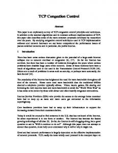
Figure 2.1: Flow diagram of the Generic Cell Rate Algorithm

2.2.3 Statistical Commitments The network guarantees to the application that it will not drop any packets of the application, or only a preset fraction of the sent packets, as long as the sending behavior of the application conforms to the negotiated values. For the ABR service, this means that as long as the application is sending its fair share and does not exceed the peak cell rate, the network will not discard any of the sent packets, or at least only a preset fraction of the sent packets.

2.3 Usage Parameter Control in the ABR Context In its September 1994 meeting the ATM Forum voted for a rate based congestion control mechanism to be used in ATM networks. With the chosen algorithm the ABR sources must send a so called resource management (RM) cell every Nrm cells. Depending on the trac situation in the network the intermediate switches can determine the fair bandwidth shares the ABR connections should use in order to avoid congestion. These values are then written in the RM cells in the explicit rate (ER) eld. The destination end system turns the RM cells around and


6 k

1 2

3

4

5 6

7

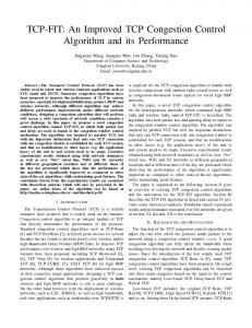
T

a

TAT

Figure 2.2: Time line for the GCRA algorithm sends them back to the source. In accordance with the explicit rate noted in the RM cells the source can then increase or decrease its rate to its fair share. To protect the network from misbehaving sources that do not reduce their rates when they are asked to do so, some kind of conformance tests must be used at the interface which can be a UNI or a NNI. Conformance indicates here that the arriving cells at the interface conform to the proper response of the sources to the RM feedback messages. In this section a de nition of this feedback conformance as it was presented in [4] is given and the generic cell rate algorithm (GCRA) that is used for testing the conformance of the arriving cells is introduced.

2.3.1 The Generic Cell Rate Algorithm The owchart in Fig. 2.1 presents the generic cell rate algorithm (GCRA) as a virtual scheduling algorithm. The GCRA is used to de ne, in an operational manner, the relationship between the sending rate and the cell delay variation (CDV) introduced by the cell multiplexing. In addition, it is used to specify the conformance of the arriving cells at the interface, e.g., UNI. For each cell arrival, the GCRA determines whether the cell is conforming with the trac contract of the connection. Here, the trac contract is used to specify the behavior the source agreed to take on during the connection establishment. The virtual scheduling algorithm updates a theoretical arrival time (TAT) which is the nominal arrival time of the cell assuming equally spaced cells when the source is active. If the actual arrival time of a cell is not too early relative to the TAT then the cell is conforming. Tracing the steps of the virtual scheduling algorithm in Fig. 2.1, at the arrival time of the rst cell Ta (1), the theoretical arrival time (TAT) is initialized to the current time. For subsequent cells, if the arrival time of the kth cell, Ta (k), is actually after the current value of the TAT then the cell is conforming and TAT is updated to the current value Ta (k) plus the increment I , with I as the inverse of the sending rate. If the arrival time of the kth cell is greater than or equal to TAT ? L but less than TAT, then again the cell is conforming and the TAT is increased by the increment I . Here, L is used to account for the cell delay variation. Lastly, if the arrival time of the kth cell is less than TAT ? L then the cell is non-conforming and the TAT is unchanged. As an example let's consider Fig. 2.2. The time axis is divided into time units , with as the time required to send an ATM cell with the peak cell rate (PCR) over the network. In this example I was set to 3 and L to 3. The rst raw of Fig. 2.2 represents the actual arrival

2.4. EXAMPLES OF TRAFFIC GENERATORS FOR ABR

7

times of the cells at the policer and the second one the calculated theoretical times. While the cells arriving up to Ta (6) are still conforming the next cell is too early and can not be entered into the network as TAT7 ? ta (7) > 3. The maximum burst size N , i.e., the maximum number of cells that can be sent at the link rate can be calculated as follows:

L j for I > N = j1 + I ?

2.3.2 The Conformance De nition

To account for the cell delay between the ABR source and its interface to the network, Berger et. al [4] suggest the usage of two delay parameters 1 and 2 that the network equipment would negotiate for the connection and the network operator could assume for the conformance de nition. These parameters would be interpreted as follows: 1 is a bound on the dierence between the maximum delay from the source to the interface and the xed component of this delay, e.g., the propagation delay. 2 is the maximum round trip time on a connection from the time when a backward RM cell on the associated backward connection with a new explicit rate crosses the interface to when the new rate takes eect in the forward cell stream arriving at the interface. Considering these two delay bounds it is proposed that the conformance de nition for ABR connection be as follows: 1. The end systems must follow the reference behavior as it was proposed by the ATM Forum in [1]. In the case of the rate based control mechanisms this would mean that a source can change its sending rate in accordance with the received messages from the network. 2. The connection must observe the delay bounds 1 and 2 for the network between the source and the interface in question. To account for this de nition, an extended version of the GCRA has to be used. With the dynamic generic cell rate algorithm (DGCRA) the time interval that is used to update the theoretical arrival time (TAT) is no longer a constant but is changed in accordance with the explicit rate noted in the feedback RM cells. If the explicit rate (ER) in the backward RM cell passing this interface is higher than the current sending rate, I is set directly to 1/ER. For rates smaller than the current rate the DGCRA algorithm should defer using the new rate until the rst cell that arrives after a lag 2 , at which point it would set T to 1/ER. This allows the interface to account for cells that were already sent with the older and higher rate and are already on the way to the interface. The interface must as well keep the rate between the minimum cell rate (MCR) and the peak cell rate (PCR). 1 replaces in this scheme the value of L that was used in the GCRA algorithm to account for the cell delay variations (CDV).

2.4 Examples of Trac Generators for ABR As already stated the ABR service is intended to be used with applications that can change their sending rate according to the available bandwidth in the network. Such applications would be usually sensitive to packet losses but can tolerate delay variations. Applications concerning


8 Active Period

Active Period Idle Period

Packet

Pause

Cells

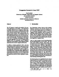
Figure 2.3: Bursty source trac model data communication are typical examples for applications that can bene t from the ABR service. Telecommunication applications like audio and video applications with their need for xed delays can hardly use this service, at least in this phase. Here, two sources that can be used for simulating applications using the ABR service are introduced.

2.4.1 Persistent Sources This kind of sources always sends with the maximum permitted rate. Dierent simulations [5] have shown that this model imposes the heaviest constraints on the network and is therefore very appropriate for testing the fairness and the throughput of the ABR service. Also, this model eliminates statistical throughput and delay uctuation that would be caused by random trac generators. Thus, it would be possible to achieve deterministic and reproducible simulation results.

2.4.2 Bursty Sources [6] describes an active/idle source that is based on a three state model, see Fig. 2.3. The source can be either in an idle or active state. While in the active state, the source generates a series of packets which are interspersed by short pauses. These packets have variable lengths and for ATM networks are themselves divided into cells that are interspersed by a minimal cell distance. The pause periods are drown from a negative exponential distribution with mean To . The number of generated packets during an active period is geometrically distributed with mean Np . The idle periods can have any distribution with mean Tidle.

2.5. GENERAL COMMENTS

9

2.5 General Comments Until now there is no nal version of the characteristics of the ABR service. The quality of service requirements and conformance de nition presented here should only be seen as work in progress. There are still many open issues for which there are still no adequate solutions. For example, it is still not clear how the resource management cells in both directions should be policed and what is their role in the overall conformance de nition. We have only described the behavior of the interface in response to the explicit rate schemes. However, as the older schemes using the EFCI marking switches should still be supported, the conformance de nition must handle this case as well. Until now, however, there is no clear de nition of how to do this. This chapter should only be seen as an overview of the current development of the ABR service. There will surely be a lot of changes done until the nal version is agreed on. The currently available ATM switches do not actually support the explicit rate behavior and there will probably be no big changes in this point until the end of 19951 .

1 According

to a private inquiry at FORE Systems.

10


Chapter 3

Congestion Control in ATM 3.1 Introduction Ensuring, at the same time, high utilization of the available bandwidth in a network with a minimum cell loss rate requires ecient as well as fair congestion control schemes. These schemes should achieve three important goals [7]: 1. At a minimum, the quality of service (QOS) negotiated during the connection establishment has to be satis ed for each source. 2. Unused bandwidth should be fairly distributed among the active connections. 3. On the occurrence of congestion the connections that are using more bandwidth than was negotiated at the connection establishment should be given the opportunity to reduce their rate before the network starts discarding trac in excess of the negotiated QoS. In this chapter dierent approaches to congestion control in ATM networks are brie y described and an attempt to compare their merits and drawbacks is made. Where possible, simulation results showing the throughput, buer requirements at the intermediate switches, and fairness performance are also provided. In our presentation of the dierent approaches to congestion control in ATM networks we relied mainly on the work done by the trac management subworking group (TMSWG) of the ATM Forum. From that work two main approaches can be distinguished: 1. Link-by-link credit based ow control 2. End-to-end rate control As the TMG voted for a rate control based mechanism in its September 1994 meeting, the credit based ow control mechanism is only brie y introduced. On the other hand, it would be tedious as well as wasteful to present every incarnation of the rate control mechanism, as there were about 10 versions or so that were merely supported by their authors. Therefore, only the main evolution steps of the rate control mechanism from the basic mechanism using bit marking to the now accepted enhanced proportional rate control algorithm (EPRCA) are described. As a compromise between the two approaches an integrated proposal is also brie y introduced. With this scheme both the credit based as well as the rate control mechanisms can be used to control the trac. 11

CHAPTER 3. CONGESTION CONTROL IN ATM

12

3.2 Credit Based Congestion Control The fundamental idea of ow control is that packets can't be sent unless the source knows that the receiver can accept the data without loss. Therefore, the receiver has to send control data to the sender with information about its available buer space. Even though that the here presented algorithm works on a hop by hop basis a correct implementation should result in a closed ow control loop.

3.2.1 Credit Based Flow Controlled Virtual Connection

The in [8] introduced credit based ow controlled virtual connection (FCVC) algorithm proposed a per VC buer and ow control. In this algorithm upstream nodes maintain a credit balance for each outgoing FCVC. Only when the credit balance for a VC is positive, the node is eligible to forward data on that VC. After sending data the credit balance is reduced. The downstream node must in return update the upstream node's credit balance by sending credit cells. These cells contain credit information re ecting the available buer space at the downstream node and are sent after forwarding N 2 cells on the VC since the previous credit cell for the same VC was sent. The N 2 parameter is a design or engineering choice. Upon receiving a credit cell the upstream node updates the credit balance for the VC. In the here introduced N23 scheme the new balance would represent the number of cells that can still be sent without over owing the receiver's buer. Destination Credit Buffer

Credit Switch

Source

Data

Credit Information Data

FC Link Upstream Node

Data Downstrem Node

Credit

Destination

Figure 3.1: Credit-based ow control

Buer Management 1. Static Allocation: In the N23 scheme of the credit based control mechanism the receiver

reserves N 2 + N 3 cells for each VC. N 3 is chosen just large enough to avoid data and

3.2. CREDIT BASED CONGESTION CONTROL

13

credit under ow. With RTT as the round trip time and BVC as the peak VC bandwidth in percentage of the link bandwidth

N 3 = RTT BVC This ensures that until a credit update cell is received at the sender all cells that were sent on that VC can be buered at the receiver. 2. Adaptive Credit Allocation: The adaptive allocation scheme avoids the need of having to specify the necessary bandwidth for a VC and reduces the amount of buer space needed for that VC. In [9] all VCs are dynamically allocated buer space from a shared buer. This is done in proportion to the actual bandwidth consumed by each VC. The actual bandwidth of a VC is calculated by counting the number of cells departing on that VC over a measurement time interval (MTI).

Performance Analysis Simulation results obtained in [10] and [11] indicate that the credit based FCVC mechanism with static memory allocation guarantees a link utilization of nearly 100%, no cell loss, minimum response time to changing load conditions and fairness towards local as well as transit trac. However, this is only reached on the expense of large enough buers. So even though the above described optimal performance can be obtained by the provision of a few megabytes of switch buer in the case of LAN links, switches in a high speed WAN environment require giga or even tera byte buers to ensure the same performance. The amount of needed buer can be substantially reduced using the adaptive allocation scheme. However, with this scheme the optimal performance reached with the static scheme is no longer guaranteed. Actually, the utilization drops to a no longer satisfactory level. Also, the response times for changing trac conditions reach unacceptable values [10]. As the bandwidth allocation policy depends on observed rates during a measurement interval and not on actual rates a source that was silent for the last MTI or a new source will only be able to increase its bandwidth share in a very slow way. Another important issue to consider is the complexity of the switches and network interface cards (NIC) needed to implement the algorithm. The static allocation version requires per VC buering and management. In the case of switches in a WAN environment with thousands of active VCs this leads to very expensive as well as complicated switches. The overall complexity of the algorithm is increased even more with the introduction of the adaptive allocation scheme. In order to maintain a zero loss rate the upstream and the downstream nodes need to maintain a consistent view of the available buer space. The need to synchronize the upstream and downstream nodes as well as the problems of how to divide the available buer and what the round trip time for the VC is lead in general to unacceptable complexity that can't be justi ed by the poor performance. The NIC is on the other hand simple to build in silicon. All SAR chips will queue packets awaiting segmentation into cells on a per connection basis. The simplest scheduler consists only of a list of connections that have packets queued for segmentation. To implement the credit based scheduler only a minimal enhancement to the existing one is needed. The scheduler should only schedule connections that have a non-zero credit balance.


14

3.3 End-to-End Rate Control In this scheme congestion information are collected along the VC's path and are conveyed back to the source end system. Based on these information the source can determine the adequate sending rate with which congestion can be avoided. In order to provide a closed end-to-end control loop, the congestion information are not sent directly to the source but are forwarded to the destination end system. This forward error congestion noti cation (FECN) provides the destination with a complete overall look of the congestion state along the connection's path. Also, it minimizes the needed number of congestion messages compared to the backward error congestion noti cation (BECN) with which each intermediate switch would send a congestion noti cation to the source end system when congestion is observed. Destination

Switch

Source

Data

Congestion Data Data Congestion Data

Buffer

Data Destination

Figure 3.2: End-to-end based rate control Here, three algorithms are introduced. They dier in their performance, complexity and the kind of congestion information conveyed back to the source. To compare between the dierent algorithms a simple generic fairness con guration [6] was chosen. With this topology, see Fig. 3.3, the fairness of bandwidth allocation can be simply tested for the case of cascaded congested links. The fairness index presented by Jain [3] with which fairness can be characterized quantitatively is used to compare between the fairness of the dierent algorithms, see Sec. 2.2. Simulation results showing rate and buer behavior of the dierent schemes are presented as well. The test network consists of four switches, with each adjacent two switches connected through a WAN link. There are four greedy sources, that send during the entire simulation with the maximum allowed rate, and four destination end systems. Except for the connection from source 0 to destination 0 that represent the transit trac in the scheme all other connections are local trac and pass only through the output buer of one switch. Except for the algorithm speci c parameters all simulations were executed with the parameters presented in Tab. 3.1.

3.3. END-TO-END RATE CONTROL Parameter ICR MCR PCR AIR Link bandwidth Link length Source link Transmission delay Congestion threshold

15

description value Initial cell rate 7.75 Mbps Minimum cell rate 0.155 Mbps Peak cell rate 155 Mbps Additive increase rate 1250 Maximum rate at which cells can leave the switch 155 Mbps Distance between two adjacent switches 1000 km Distance from the source to the switch 0.4 km Delay caused by the physical medium 5 sec/km Allowed buer length at the switch 50 cells

Table 3.1: Simulation parameters for testing the rate control algorithms

Each link is shared between two connections with the same requirements, the same MCR and dier only in their round trip time, so that the fair share for each connection can be determined with the Max-Min fairness criteria presented in Chapter 2. With this in mind the fair share for each connection would intuitively be half of the link's bandwidth, i.e., 77.5 Mbps or 182783 cells/sec. The buer requirements in all the switches and the rate dynamics for the local sources, source 1, source 2 and source 3, show more or less the same behavior with negligible variations. The only dierences noticed stem from the delayed arrival of the transit cells at the switches. Therefore, only the results of the buer requirements of the rst switch and the relation between the local connection from source 1 to destination 1 and the transit connection from source 0 to destination 0 are shown.

Destination 1

Destination 2

Destination 3

Destination 0

Source 0

155 Mbps

Switch 1 0.4 km

1000 km Switch 2

Switch 3

155 Mbps

Source 1

Source 2

Source 3

Figure 3.3: The generic fairness con guration

Switch 4


16

3.3.1 Rate Control Using EFCI Marking

This simple algorithm uses the explicit forward congestion identi cation (EFCI) bit in the payload eld of the cell header to determine the congestion state of the network [12]. 1. Source End System Behavior The source starts sending cells with the initial cell rate (ICR) that was de ned at connection establishment with the EFCI state set to not congested (EFCI=0). The rate is changed in so called update intervals (UI). Receiving a resource management (RM) cell during an update interval, indicates congestion and causes a rate reduction by the multiplicative decrease factor (MDF) which was set to 0.875 due to a recommendation in [5]. The rate is additively increased by the additive increase rate (AIR) after an update interval in which no RM cells were received. If a source remained idle for an update interval then its rate is multiplicatively decreased as well. Increasing and decreasing the rate has to be done in such a manner that the PCR is not exceeded and the rate does not go below MCR. 2. Switch Behavior Switches use the switch buer length as an indication of congestion. Exceeding a preset congestion threshold in an intermediate switch, i.e., the switch buer gets longer than a pre de ned length, causes the switch to mark the EFCI bit in all incoming cells to congested. 3. Destination End System Behavior The destination end system determines the congestion state in the network through the EFCI state in the received cells. If congestion was observed or internal congestion existed a RM cell has to be sent. As long as the internal congestion lasts and no cells with (EFCI=0) are received an RM cell has to be sent every resource management interval (RMI). This interval is, just like the update interval at the source end system, determined through a timer.

Simulation Results Other than the parameters mentioned in Tab. 3.1, Tab. 3.2 lists the values of algorithm speci c parameters used for this simulation: Parameter MDF UI RMI

description value Multiplicative decrease factor 0.875 Update interval 0.0002 sec Resource management interval 0.0001 sec

Table 3.2: Simulation parameters for the EFCI marking algorithm 1. Evaluation of the buer requirements The number of cells in the switch buer is bound to accumulate whenever the sum of the sending rates of the connections passing this switch is higher than the link service rate at the switch. This means that in our case, whenever the sending rate of the local source

3.3. END-TO-END RATE CONTROL

17

plus the sending rate of the transit source get higher than 155 Mbps each additional rate increase causes the buer to build up at the switch. To simplify the coming calculations we will consider the link service rate at the switch as 0 Mbps and that the sources are increasing their rates from 0 as well. The simplest way to get a rough estimation for the resulting buer length would be to consider the time axis as divided into sending intervals. Each interval should be just long enough for the rate increase done in that interval to result in the sending of an additional cell. As an example for this consider a source that increases its rate by 1 cell/sec. This results in an interval with the length of 1 second with one cell sent in the rst second, two cells in the second one and so on. The length of the interval can be calculated as follows: 1 = UI n AIR n With AIR and UI having the values from Tab. 3.1 and 3.2 and n as the number of needed update intervals to cause a rate increase of one cell per sending interval. Here, n can be calculated to 6.3. As we can only consider complete update intervals the sending rate is calculated as UI jnj = 0:0002 7 = 0:0014 sec The buer build up phase can be divided into two periods: (a) In the rst period the buer builds up until it reaches the congestion threshold. As both sources increase their rates in the same way they will also contribute in same way to the buer build up. This means that with the threshold set to 50 cells the switch will start marking the EFCI bits after each source has sent 25 cells. At the time that this happens each source will have increased its rate to m cells per sending interval. m can be calculated as follows: m X i = 25 i=1

This results in m 7, i.e., when reaching the congestion threshold each source would be sending at a rate of 7 cells per sending interval. (b) After the rst EFCI bit is marked congested it would take a complete round trip time until the eects of the rate reduction at the source show at the switch. In our model the round trip time for the local source is 0.01 sec. This equals to approximately 7 sending intervals in which the source can still increase its rate. During these 7 sending intervals each source cause the buer length at the switch to increase by:

X i = 77

7+7 i=7

In other words the local source will send 77 + 25 = 103 cells before reducing its rate. Now depending on the used reduction factor the buer build up will only last until the rate reduction at the local source compensates for the rate increase at the transit source which has a longer round trip delay time.


18 250

Length (Cells)

200

150

100

50

0 0

0.2

0.4

0.6

0.8 1 Time (sec)

1.2

1.4

1.6

1.8

Figure 3.4: Switch buer requirements as a function of time for the EFCI marking algorithm This simple calculation shows that until the rate reduction at the local source takes eect both sources will cause a buer of about 206 cells at the switch.

2. Buer requirements Fig. 3.4 reveals that even though the congestion threshold was set to 50 cells around 230 cells of switch buer were needed to ensure lossless trac. This value con rms our theoretical evaluation of the needed buer at the switch 3. Fairness The high oscillation of the throughput of both the local as well as the transit connections, as can be seen from Fig. 3.5, leads to the low utilization of 54%. Both connections shown in the gure share the utilized bandwidth in an increasingly unfair way. Whereas the local source received 52% of the utilized bandwidth during the measured interval, only 48% of the bandwidth were allocated to the transit trac. This results in a fairness index of 0.99 which is actually very good. Fig. 3.5 shows, however, that these values are misleading. The throughput of the local source is increasing while the share of the transit trac is actually decreasing. So, while the transit connection received in the rst second of the simulation about 50% of the utilized bandwidth its share decreased to around 48% of the bandwidth in the last second of the simulation. This implies that a longer simulation would result in a much smaller fairness index.

3.3.2 Proportional Rate Control Algorithm

The proportional rate control algorithm (PRCA) is based on the positive feedback rate control scheme [13]. In this scheme the rate can only be increased if a positive indication, in this case a RM cell, to do so was received. Otherwise, the rate is continually decreased after each sent cell.


19

106 Transit source Local source

Throughput (Cells/sec)

105

104

103

102 0

1

2 Time (sec)

3

4

Figure 3.5: Rate with EFCI marking Rate reductions and increases are done in proportion to the current sending rate. This not only enhances the fairness of the rate control scheme compared to the previous algorithm, but also eliminates the need for timers as they were needed in Sec. 3.3.1. 1. Source End System Behavior The source starts sending cells at an initial cell rate (ICR) with the EFCI state set to congested (EFCI=1). In the rst cell and every other Nrm cells EFCI is set to 0. Here, Nrm was set to 32 due to a recommendation of the ATM Forum. Each cell with (EFCI=0) represents an opportunity for the source to increase its rate. If these cells faced no congested links along their entire path a RM cell will be generated at the destination end system. On receiving these RM cells the source is entitled to increase its rate. This is done in such a manner as to compensate for all the decreases taken over the last Nrm cells and to achieve the desired overall rate increase. After the sending of each cell the rate is multiplicatively decreased by the multiplicative decrease factor (MDF). 2. Switch Behavior A congested switch can indicate its congestion state in one of the following two ways:

Set the EFCI state in the passing cells to congested (EFCI=1). Remove RM cells generated by the destination end system and sent on the backward direction to the source while the congestion lasts on.

3. Destination End System Behavior If a cell is received with (EFCI=0) and no internal congestion is noticed the destination end system sends a RM cell to the source.


20

Simulation Results To simulate the behavior of the PRCA proposal the generic fairness topology presented in Fig. 4.5 was used with the parameters of in Tab. 3.1 and the algorithm speci c parameters of Tab. 3.3. Fig. 3.6 shows that to guarantee lossless trac using the PRCA proposal the switches need buers that could reach about 1050 cells long. This value is clearly much larger than the 230 cells needed with the EFCI marking algorithm. Parameter description value 1 MDF Multiplicative decrease factor 8 Nrm Number of data cells that can be sent before sending a cell with EFCI=0 32 Table 3.3: Simulation parameters for the PRCA algorithm The most important result that can be taken from Fig. 3.7 is the severe unfairness of the algorithm. Whereas the local connection, source 1 to destination 1, manages to transport 183594 cells in 1.59 seconds, only 118805 cells get transported in the same time period over the transit connection from source 0 to destination 0. This means that at a link utilization of only 53% the local connection gets around 60% of the utilized bandwidth. In terms of the fairness index this results in a 0.94 fairness. 1.2⋅103

103

Length (Cells)

800

600

400

200

0 0

0.2

0.4

0.6

0.8 1 Time (sec)

1.2

1.4

1.6

1.8

Figure 3.6: Switch buer requirements as a function of time for the PRCA algorithm 1 Rate

reduction in this algorithm is done in the form of ACR = ACR ? 2ACR MDF :


21

3.5⋅105 Transit source Local source


3⋅105 2.5⋅105 2⋅105 1.5⋅105 105 5⋅104

0 0

0.2

0.4

0.6 0.8 Time (sec)

1

1.2

1.4

Figure 3.7: Rate with PRCA

3.3.3 Enhanced Proportional Rate Control Algorithm

The enhanced proportional rate control algorithm (EPRCA) provides two major enhancements to the PRCA proposal presented in [13]: Explicit rate indication: Here, the sources receive an explicit indication of their fair share of the bandwidth which they should use in order to avoid congestion. Intelligent marking: With this approach only the rates of greedy connections that caused the congestion are reduced. This is done by denying these connections the opportunity to increase their rates. To implement these enhancements the source end systems have to generate RM cells every Nrm sent data cells and write their current rates in them. At the intermediate switches the fair rate share of each source is calculated and written in the RM cells. The destination end systems send the RM cells back to the originating sources. If the intelligent marking was used the switches can set a congestion bit in the RM cells passing over the backward stream of the high rate connections and thereby denying these connection the opportunity to increase their rates. The RM cells have to at least carry the following parameters [14]: ACR: The allowed cell rate is used mainly to selectively indicate congestion on connections passing a congested link. That is, intermediate networks can signal VCs with a high ACR to reduce their rates while allowing other connections to keep their current rates or even increase them. Thereby, fair allocation of rate among competing connections can be ensured. ER: The explicit rate is initially set to the peak cell rate and can be modi ed downward by intermediate switches to the adequate rate needed to avoid congestion.

22


CI: With the congestion indicator compatibility to older switches using EFCI marking can

be provided. CI is set to congested (CI=1) in the backward sent RM cells at the destination if the EFCI state in the last received cell indicated congestion. Intermediate switches can also set CI in the backward RM cells if congestion was observed on the forward direction for that VC. DIR: Direction of the RM cell, backward or forward relative to the source.

1. Source End System Behavior The source starts sending cells at an initial cell rate (ICR) with EFCI set to 0. Each Nrm data cells a RM cell is generated with CI=0, ER=PCR and DIR=forward. After each sent data cell the rate has to be reduced by the multiplicative decrease factor (MDF). EPRCA is, just like the PRCA proposal, based on the positive feedback scheme. That is, a source can only increase its sending rate when a positive indication is received from the network. Positive indications are included in the RM cells and depending on the congestion mode used can take one of the following two forms: In the intelligent marking mode a received RM cell with (CI=0) indicates that the network is not congested and that the rate can be increased. The ER value in the received RM cells indicates in the explicit rate indication mode the rate that the source should take on to avoid congestion. 2. Switch Behavior In the EPRCA scheme congestion can be indicated in one of the following two modes: (a) Intelligent marking: Connections which advertise a high ACR value in their RM cells are signaled to reduce their rates. This can be done through setting the CI bit in the backward RM cells for that VC. Unlike the PRCA proposal which reduces the rate of all sources this scheme allows connections with low ACR to increase their rate and hence ensures a fair allocation of the bandwidth. (b) Explicit rate indication: This algorithm is based on determining the advertised rate (A-rate) as was presented by Anna Charny in [15]. Based on that the fair rate a switch should advertise is the capacity available minus the capacity of the constrained VCs over the total number of VCs minus the number of constrained VCs. P Bandwidth of link ? Bandwidth of connections bottlenecked elsewhere P Number of connections ? Number of connections bottlenecked elsewhere However, as most of the used values in this equation are not directly known another method has to be used to determine the A-rate. As the A-rate is actually the average rate of all connections that face no constraints on any part of their paths [16] presents a heuristic scheme that tries to estimate the fair bandwidth share via an estimation of the exponential average. To ensure that the estimated average and ACR converge to some stable value under all conditions several multiplier factors were added to the algorithm to force convergence. The following pseudo code was taken completely from [16] and presents the basis for the switch behavior used in various simulation studies [17].


23

Initialization MACR=IMR !Initialize MACR to a small rate. FOR Each RM Cell Received at the Switch IF receive RM(ACR,DIR=forward,ER,CI) IF (Congested and ACRMACR*VCS) MACR=MACR+(ACR-MACR)*AV ! Average ACR's IF receive RM(ACR,DIR=backward,ER,CI) IF Congested IF Q>DQT ! Test queue length to see if it was very congested IF mode=Binary THEN CI=1 ! Set Congested bit IF mode=explicit THEN ER= min(MACR*MRF, ER) ! Major reduction ELSE IF ACR>MACR*DPF !Select VC's for congestion marking IF mode=binary THEN CI=1 ! Set Congestion bit IF mode=explicit THEN ER= min(MACR*ERF, ER) ! Reduce rate

The following explanation and initialization of the parameters that were used in the algorithm were, just like the pseudo code, taken completely from [16]. The values chosen for the parameters were determined from simulations and experiments done by L. Roberts and were not further tested during this work. MACR: Congestion point rate computed by the switch as an approximation of the exponential average. Q: Queue length in cells at the switch. Congested: State of congestion of the queue typically determined by a threshold. IMR: Initial rate for MACR. Used only on start-up and is set to IMR = PCR=100:

VCS: VC separator. The VC separator is to separate the otherwise bottlenecked VCs from the VCs constrained at this switch. It should be of the form 1 ? 2n and is set here to

VCS = 7=8: AV: Average factor. This has worked best at 1/16. For large numbers of VCs, it should be reduced. However, the smaller the factor the slower the switch converges to overload and the more buer space is needed. It should be of the form 2n and is set here to AV = 1=16:


24

DQT: High queue limit to determine the very congested state. It should be set

well above the threshold used to determine normal congestion and is initialized to DQT = 300 cells. MRF: The major reduction factor is used to rapidly decrease the queue length during the very congested state. It is of the form 2n and is set to MRF = 1=4:

DPF: The down pressure factor reduces the testing mark for the ACR. It is of the form 1 ? 2n and is set to

DPF = 7=8: ERF: The Explicit reduction factor is used to set the explicit rates slightly below MACR so that the switch will stay uncongested. It is of the form 1 ? 2n and is set to ERF = 15=16: This implementation has proved to be accurate as well as simple. Using the MCRA eliminated the need for a VC table as was suggested by Anna Charny in [15]. The implementation of the fair share calculation algorithm presented here has to be seen only as one possible solution that proved to work ne. As the switch speci cs will not be standardized by the ATM Forum the actual used algorithm can take any other shape that ful lls the fairness requirements, for example see [18]. Actually, this implementation is calculation intensive and would not be ecient in a real switch. The switch must update the MACR value every received forward RM cell and write the explicit rate in the backward RM cells. At a link rate of 155 Mbps and Nrm set to 32, 11424 RM cells/sec would be sent on each direction. This would lead to complex as well as expensive switches. 3. Destination End System Behavior On receiving a RM cell the destination host generates a new RM cell with DIR set to backward and ER and ACR set to the values of ER and ACR in the received RM cell. To ensure compatibility to older switches using EFCI marking the destination has to keep track of the EFCI state in the received cells. If the last received cell had EFCI set to congested then CI in the backward RM cell has to be set to 1. Otherwise, CI gets the value of CI in the received RM cell.

Simulation Results Just like the last two simulation experiments the EPRCA proposal was tested with the generic fairness topology from Fig. 4.5 and the parameters of Tab. 3.1. In addition to that, some algorithm speci c parameters that were used are depicted in Tab. 3.4. Calculating the fair rate share for a connection and writing it in a RM cell is certainly more complicated than just setting a congestion bit, as was done in Sec. 3.3.1 and Sec. 3.3.2. But it actually leads to an optimal rate allocation as well as reducing the oscillation to a minimum.


25

Also the impact of the initial rate can be eliminated more quickly. The source can start at link rate and the overload will last for only one round trip. In a bit based scheme like the EFCI marking and the PRCA proposals a source would require several round trip times before converging to the optimal value. Parameter description value 2 MDF Multiplicative decrease factor 8 Nrm Number of data cells that can be sent before sending a RM cell 32 Table 3.4: Simulation parameters for the EPRCA algorithm Whereas the last two algorithms only reached a network utilization of about 50% under the given condition of low buer usage the EPRCA proposal provided high utilization, low buer requirements and fair bandwidth allocation under various topologies, see also [17]. The high utilization during the steady state (around 97%) and the fair rate allocation can be clearly seen in Fig. 3.9. In the steady state the transit connection gets 49% of the utilized bandwidth and a fairness index of about 0.994 can thereby be reached. Fig. 3.8 shows that the maximum buer needed to ensure lossless trac is about 70 cells only. 80

Length (Cells)

60

40

20

0 0

0.1

0.2

0.3

0.4

0.5

Time (sec)

Figure 3.8: Buer requirements as a function of time with the EPRCA algorithm 2 Rate

reduction in this algorithm is done in the form of ACR = ACR ? 2ACR MDF :


26 3⋅105


2.5⋅105

2⋅105

1.5⋅105

105

5⋅104 Transit source Local source 0 0

0.1

0.2

0.3 Time (sec)

0.4

0.5

0.6

Figure 3.9: Rate with EPRCA

3.3.4 Results Evaluation Tab. 3.5 summarizes the main results obtained from simulating the three rate control algorithms discussed in this chapter. It is obvious that the decision of the ATM Forum to chose the EPRCA proposal for congestion control over ATM is correct. Under the given topology this algorithm achieved the highest bandwidth utilization and the fairest allocation with the lowest buer requirements. Algorithm fairness index link utilization maximum buer needed at the switch EFCI 0.99 54% 230 cells PRCA 0.946 53% 1050 cells EPRCA 0.994 97% 70 cells Table 3.5: A general comparison between the results of the tested algorithms However, the results reported for the PRCA and the EFCI marking proposals only give an incomplete representation of their actual performance. The high oscillations of the throughput of the PRCA proposal and the low utilization caused thereby were mainly forced by the small congestion threshold. In another simulation using a congestion threshold of 3400 cells the oscillations are considerably reduced, see Fig. 3.10, and the utilization reached 94.5% of the available bandwidth. The unfairness presented in Sec. 3.3.2 is, however, still obvious. While the local trac consumed about 76.8% of the utilized bandwidth the transit tracs bandwidth decreased to 23.2%. This resulted in a fairness index of only 0.817.


27

4⋅105


3⋅105

Transit source Local source

2⋅105

105

0 0

0.1

0.2

0.3 Time (sec)

0.4

0.5

0.6

Figure 3.10: Throughput of the PRCA proposal with the congestion threshold set to 3400 cells

Fairness Fairness is a central issue in the congestion control discussion. The credit based algorithms were even, for a while, favored over the rate based solutions mainly because of the inherent unfairness of the rate based solutions using EFCI marking for congestion identi cation, see Sec. 3.3.1 and 3.3.2. Parameter MCR PCR AIR UI RMI Link delay Congestion threshold

description value Minimum cell rate 0.155 Mbps Peak cell rate 155 Mbps Additive increase rate 1250 Update interval 0.002 sec Resource management interval 0.001 sec Propagation delay between two switches 0.005 sec Allowed buer length at the switch 300 cells

Table 3.6: Simulation parameters for testing the eects of dierent MDF values The problem of unfairness in the EFCI marking proposal stems from the way the sources are noti ed about congestion. This proposal does not dierentiate between fast sources that are the cause of the congestion and slow sources that should be allowed to at least keep their low rate. In the case of congestion all sources are noti ed to reduce their rate every RM interval until the network is no longer congested. As the rate reductions are done in a multiplicative manner we could expect the rates for both sources to sooner or later converge to the same value. This depends on the chosen reduction factor and update interval. However, until the sources converge


28

the bandwidth will be unfairly distributed and the source with the higher initial cell rate will receive a much higher share of the bandwidth. The length of this transient period depends on the used reduction factors. Smaller MDF values cause a more rapid reduction and a shorter transient period, thereby leading to a fairer bandwidth allocation. However, the utilization will suer from the rapid reduction of rates. To demonstrate the eects of the value of the reduction factor a few simulation runs were made using the simple network topology depicted in Fig. 3.11. Two sources with the same Destination0 Source0

Congested Link Switch1

Switch2

Source1

Destination1

Figure 3.11: Test network initial parameters, see Tab. 3.6, and the same round trip delays but with dierent initial cell rates, share a common link. Source0 starts sending with the peak cell rate and Source1 has an initial cell rate of 7.75 Mbps. A fair congestion control algorithm should allocate both sources the same bandwidth. Three simulation runs were made with MDF = 0.9, 0.85 and 0.75. As can be seen from Fig. 3.12 the anticipated behavior is achieved. The two sources start sending at dierent rates and pass through a transient period in which they send at dierent rates until their rates converge to the same value. Reducing the value of MDF causes the duration of the transient period to decrease and the utilization over the measured period to drop, see Tab. 3.7 . MDF utilization length of the transient period 0.9 75% 1 sec 0.85 68% 0.8 sec 0.75 59% 0.5 sec Table 3.7: The eects of MDF on utilization and fairness using the EFCI marking algorithm Another important observation is the behavior of the rates in the steady state. With higher MDF values the throughput shows smaller oscillations and on the average a higher value. This indicates that the MDF value should be carefully chosen in order to ensure high utilization and fair rate allocation. The inability of the algorithm to distinguish between fast and slow sources is only in part responsible for the unfairness of the algorithm. A more severe problem is the unfairness towards connections with longer round trip delays, as can be seen from Fig. 3.5. This problem is common among all EFCI marking switches, i.e., also with the PRCA proposal, see Fig. 3.7. As the transit trac passes more than one congested link it will suer a longer congestion period than trac passing only over one link. For the generic fairness con guration used here for comparing the


29


Throughput with MDF=0.9 4⋅10

5


3⋅105 2⋅105 105 0 0

0.2

0.4

0.6

0.8 1 Time (sec)

1.2

1.4

1.6

1.8

1.4

1.6

1.8

1.4

1.6

1.8


Throughput with MDF=0.85 4⋅10

5

3⋅105 2⋅105 105 0 0

0.2

0.4

0.6

0.8 1 Time (sec)

1.2


Throughput with MDF=0.75 4⋅105 3⋅105 2⋅105 105 0 0

0.2

0.4

0.6

0.8 1 Time (sec)

1.2

Figure 3.12: Throughput of Source0 and Source1 under dierent MDF values with the EFCI marking algorithm dierent algorithms this can be explained through the following scenario: As the transit trac will reach the intermediate switches at dierent time points due to the link delay the switches will go into the congested state at asynchronous time points. Also, the uncongested state will be reached in an asynchronous manner. So, for example, if the rst switch moved from the congested state to the uncongested one it will stop marking the EFCI bits in the passing cells. This would allow the local source to increase its rate. The transit trac on the other hand will still have to pass other links that are still congested and more EFCI bits will be marked for this trac. This results in longer congestion periods for the transit trac and a more severe reduction of its rate. To account for this unfairness the results obtained from the previous discussion of the reduction factors can be used. To compensate the longer congestion period, the transit connection could use a less aggressive reduction factor. For the PRCA proposal we have used the generic fairness con guration with a congestion threshold of 3400 cells and the MDF for the transit source set to 10 and 16 instead of 8. The throughput


30

Throughput with MDF of the transit source= 16 6

10



10

Throughput with MDF of the transit source= 10 6

105

104

105

104

Transit source Local source 103

103 0

0.2

0.4 Time (sec)

0.6

0.8

0

0.2

0.4 Time (sec)

0.6

0.8

Figure 3.13: Throughput of a local source and the transit source with MDF=10, 16 of the local source and transit source are depicted in gure 3.13. The transit source receives now a much higher share of the bandwidth. Setting MDF 10 results in an optimal bandwidth distribution with each source receiving 50% of the bandwidth. With MDF set to 16 the transit connection receives even four times as much as the local one with the utilization around 83%. The unfairness towards the local source indicates that we have chosen a much too large MDF and that a smaller value would have been probably enough. The EPRCA proposal avoids all of these problems by calculating the fair rate share and setting the source rate to that share. Thereby, the eects of longer congestion periods and faster and slower sources are eliminated as each source can raise or lower its rate to the correct share. With this approach the fairness can be guaranteed with a high utilization without the need to change factors in dependence of the round trip time or network con guration.

Buer Requirements In spite of its very high link utilization, fairness and the relative simplicity of the needed NICs the credit based algorithm was rejected by the ATM Forum in part due to its large buer requirements. The simulation results presented in the previous sections show the buer requirements for the rate based control algorithms to be moderate and acceptable compared with the buers needed with the credit based solutions. However, those results were based on sources that start sending with an initial cell rate that is less than their fair share and put thereby no constraints on the switch buer during the transient phase. In this section we have run the same simulations as before again, i.e., using the generic fairness con guration and the parameters of Tab. 3.1 but with the initial cell rate of all sources set to the peak cell rate which should result in the highest


31

104

Length (Cells)

103

102

101

100 Buffer of Switch1 with EPRCA Buffer of Switch1 with PRCA Buffer of Switch1 with EFCI 10−1 0

0.05

0.1 Time (sec)

0.15

0.2

Figure 3.14: Buer requirements at the switch with ICR=PCR buer requirements. Fig. 3.14 reveals that the PRCA and EPRCA proposals handle this case with no problems. The PRCA scheme requires no more than 80 cells of buer at the switch which is by far less than its buer requirements during the steady state. The EPRCA needs about 110 cells. The EFCI marking proposal needs on the other hand more than 6500 cells to ensure lossless transmission. This dierence in performance stems from the way the algorithms control the sending rates. The EFCI marking algorithm tries to increase the sending rate after each update interval in which no RM cells were received. This means that the sources can keep on sending with the peak cell rate at least until the rst RM cell is received. This can however only occur after a whole round trip time. Ensuring lossless trac in this case would require a very large buer even compared to the credit based algorithm. Each switch would have to provide at least the following amount of buer:

Pn

i=1 Ri

RTTi with n = Number of active connections RTTi = Round trip delay of connection i Ri = Peak Cell Rate - fair bandwidth share of connection i

The PRCA and EPRCA reduce the sending rate after each sent cell until a positive indication is received from the network. Hence, the congestion will only last until the sum of the rates over a connection becomes less than the link bandwidth. The length of this transient period depends mainly on the used reduction factors. The dierence between the buer requirements of the two algorithms stems from the way the reduction factor is controlled. While with PRCA proposal the reduction factor is calculated anew only after the reception of a RM cell the EPRCA proposal changes the reduction factor every Nrm sent cells. As the additive reduction factor depends linearly on the current rate and the rate itself gets reduced after every sent cell the value of


32

the reduction factor will be reduced with every new calculation. Also out of band RM cells are generated every Nrm data cells, thus adding further constraints on the buer. This value is, however, not of global meaning and should not be seen as a nal representation of the EPRCA proposal. There are still lots of discussions about the behavior of the EPRCA end systems and the way the rate should be reduced. Our version depends on the source code presented in September 1994 and until a nal version is agreed on a true characterization of the behavior will not be possible. For a detailed analytical description of the buer behavior and requirements of the EPRCA and the PRCA proposal see [19].

Management Overhead In order for the source end systems to regulate their rates they need congestion information from the network. These information are conveyed to the source through so called resource management cells. For the simulation series done in Sec. 3.3.4, the percentage of the generated RM cells compared to the number of data cells that were carried on each connection was calculated. The results are presented in Tab. 3.8. Algorithm EFCI PRCA EPRCA

RM cells for the local source RM cells for the transit source generated RM cells sent data cells generated RM cells sent data cells 0.34% 0.73% 1351 397695 2693 370776 2.6% 2.5% 5170 195761 3141 127263 6.25% 6.25% 8041 128611 6153 98426

Table 3.8: Management overhead due to the generation of RM cells Taking a brief look at Tab. 3.8 con rms the expectations that: 1. The number of generated RM cells for each connection with the EFCI marking proposal varies between a maximum of Simulation time Resource Management Interval for congested networks and 0 for networks that suer no congestion during the whole lifetime of the connection. 2. For the PRCA proposal the number of RM cells used by each connection can vary from a maximum of Transmitted Cells Nrm for networks that suer no congestion during the entire life time of the connection and 0 for congested networks.

3.4. INTEGRATED PROPOSAL FOR ABR SERVICE CONGESTION CONTROL

33

3. For the EPRCA proposal the bandwidth loss due to management overhead is 2*Transmitted Cells Nrm where Nrm was set to 32 as recommended in [16]. Even though this is much higher than that for the other algorithms it has to be taken into consideration that the overall bandwidth gain with this proposal covers this loss and is thereby justi able. Comparing the absolute number of generated RM cells for the local as well as the transit trac con rms the observations done in Sec. 3.3.4. There, we mentioned that the unfairness of the algorithms based on EFCI marking switches towards transit trac stems mainly from the longer congestion periods this trac faces with the increased number of switches. For the EFCI marking proposal this can be directly seen from the fact that the transit source receives far more RM cells than the local source. For the PRCA proposal the number of received RM cells at the transit source is less than that for the local source. As the RM cells represent here an opportunity to increase the rate the transit source will have an overall throughput less than that of the local source.

3.4 Integrated Proposal for ABR Service Congestion Control The credit based proposals have proven to be very ecient with reasonable buer requirements and simple network interface cards when used in LAN environments. However, in a WAN environment with a much larger number of VCs that must be controlled and the larger round trip times the complexity of the switches and their buer requirements grow out of control making the implementation of the algorithm too expensive. The current rate control based algorithm (EPRCA) has shown similar performance to that of the credit based algorithm with reasonable complexity and buer requirements. With the EPRCA algorithm the NIC has to control the sending rate and adjust it according to the messages received from the network. This results in a more complicated as well as expensive NIC. As the cost issue is of main importance when introducing the ATM to the LAN community the more expensive NICs could represent a handicap to ATM in its race with advanced LAN technologies like fast-Ethernet. With this in mind Singer et al. [20] presented an integrated solution that proposed the following points: To de ne a congestion control interface between subnetworks. A subnetwork is in this case a group of entities that share a common control algorithm. That a default rate control algorithm be de ned that all entities at the subnetwork interface must implement. That an auto con guration method be de ned, which allows two entities to use a non default control algorithm. However, having dierent control algorithms deployed on dierent subnetworks would invoke interoperability problems and would make the access to WANs and public networks more expensive. As the end users will surely choose a NIC that can only do rate or credit control and

34


not a more expensive version that is capable of both, the switches will have to incorporate both mechanisms. This will increase the switch costs and thereby the access costs from one subnet to another. Another problem that should be considered is that the standardization process for a mechanism is usually very dicult and long. By having to standardize two mechanisms, the nal speci cation of the UNI will take even longer and hence further delay the introduction of ATM.

Chapter 4

A TCP Simulator with PTOLEMY 4.1 Introduction Even though lots of TCP simulators and TCP trac sources are already implemented in dierent programming languages, e.g., REAL [21], the x-Kernel [22], tcplib[23] , we have decided to implement our own simulator. Building a simulator with PTOLEMY [24] would not just ease the integration and handling of the simulator as a TCP trac source in general, but would add a very useful galaxy to PTOLEMY as well. For this reason two versions of a 4.3BSD Tahoe based TCP simulator were implemented. The basic version provides the user with the usual TCP-window based control mechanism, as well as the slow start, congestion avoidance and round trip estimation algorithms suggested by Jacobson [25]. In the enhanced version of the simulator the fast retransmission algorithm was implemented as well. It will be shown that with this enhancement the throughput and performance of the protocol increases considerably since the number of retransmitted packets decreases. To verify the simulator and to compare the two versions a network con guration has been chosen that has already been used in another study [26]. Whereas the results obtained from both simulators show a great similarity to the ones reached in [26], the basic version shows a reduced eciency.

4.2 A Brief History of TCP Before moving to the actual simulator implementation and the description of its dierent features this section summarizes the basic development of TCP. 1. 4.2BSD (1983): The rst widely available release of TCP/IP based on RFC 793 [27]. 2. 4.3BSD Tahoe (1988): The version implemented here. The main protocol improvements introduced were slow start and congestion avoidance algorithms. 3. 4.3BSD Reno (1990): This implementation increased the eciency of the protocol through a better implementation. The main changes like TCP header prediction, and more eective silly window handling code increased the speed of the sender but did not 35

36

CHAPTER 4. A TCP SIMULATOR WITH PTOLEMY alter the protocol itself. Other changes aimed at reducing the spurious retransmissions through invoking slow start on idle links and a better accounting for the variance of the round trip time in the round trip time estimation, for more information see [28]. 4. 4.4BSD (1993): To allow TCP to perform well over the so called long fat pipes, i.e., links with large bandwidth-delay products, a few new options had to be included. These options allow for window size scaling, protection against sequence number wrap up and a better round trip time estimation, as described in RFC 1323 [2]. 5. 4.3BSD Vegas (1994): Here an improved round trip time estimation algorithm is used and the congestion avoidance and slow start mechanisms were modi ed [29].

4.3 4.3BSD Tahoe TCP Congestion Control Algorithm The Reno TCP release was mainly intended to improve the performance of the hosts. This was done without altering the protocol or adding any new algorithms to the Tahoe version. Since we can assume the simulated hosts to be perfect hosts, i.e., hosts that consume no time while processing packets or executing the control algorithms, there was no need to implement the changes introduced by Reno. The options introduced in RFC 1323 allow for a 32 bit long representation of window sizes and sequence numbers, which is more adequate for high speed networks. As window sizes and sequence numbers are represented as integers in the simulator these options are already implicitly contained in the implementation. The improved round trip time estimation introduced in RFC 1323 is on the other hand discussed in Appendix A. With Vegas the behavior of the sending host has been altered in order to improve the overall performance. These changes are however still under discussion and are not included in what can be called a typical TCP implementation. As our aim was to implement a basic TCP model that includes the main features of the congestion control algorithm without wasting time on unnecessary or not yet standardized improvements or extensions we chose to implement the Tahoe version. This version includes explicitly the main services of the congestion control algorithm of TCP. Implicitly some of the desired extensions like the usage of windows larger than 64 kbytes are added to the simulator through the implementation itself. In this section a brief description of the services provided by the simulator are introduced and the dierences between the two versions are mentioned. As there is no interest in using the simulator as a real TCP source, some simpli cations have been taken during the implementation:

Instead of using the usual TCP clock with a resolution of 500 msec the time information were taken from the timestamps of the packets. These timestamps had to be added to the packets anyway as the discrete event scheduler of PTOLEMY uses these stamps to determine the right sequence of scheduling. The resolution of the clock can however be determined by the user. This not only leads to an easier implementation but to more precise results as well.

All packets have the same length which is the maximum segment length (MSS).

4.3. 4.3BSD TAHOE TCP CONGESTION CONTROL ALGORITHM

37

A packet consists only of a header that contains elds describing the source and destination addresses, size of the packet, a packet sequence number, a byte sequence number and an acknowledgment eld.

A connection always exists, i.e., there is no need for a connection establishment and termination phase.

Only congestion related and necessary mechanisms were implemented, i.e., no PUSHFLAG, urgent mode, or persist timer.

In what remains of this section the implemented algorithms are brie y described. For more detailed information, see [30]. 1. Sliding window: On the arrival of a data packet at the receiver, an acknowledgment for the last correctly received byte, is generated. The acknowledgment also contains information about the amount of data the source could still transmit without congesting the receiver, the so called advertised window. The source can now keep on sending data until the sequence number of the last sent byte equals the sum of the last acknowledged byte number plus the advertised window size. 2. Silly window handling: The silly window handling mechanism is used to avoid the exchange of small data segments. This can occur due to the advertisement of small windows instead of waiting until a larger window can be advertised. At the source side this can occur due to the sending of small segments instead of waiting for additional acknowledgments. Whenever the size of the advertised window drops below the MSS a window of size zero is advertised. An update packet is then sent when the size of the advertised window reaches half of the maximum window size. 3. Slow start: The slow start algorithm adds another local window to the TCP source, a congestion window (cwnd) that is measured in segments. When a packet is lost or when a new connection is established, this window is set to the size of one segment. Each time an acknowledgment is received the cwnd is increased by the size of the acknowledged segments. The source can now transmit up to the minimum of the cwnd and the advertised window. 4. Congestion avoidance: Through the exponential increase of the sending rate caused by the slow start algorithm, the capacity of the network will be reached at some time and an intermediate router will start discarding packets. In order to avoid this the slow start algorithm was supplemented through the congestion avoidance algorithm. With this algorithm the congestion window is increased for each acknowledgment as follows: 1 cwnd + = cwnd This way the congestion window increases by at most one segment each round trip. The relation between the congestion avoidance and the slow start will be explained when discussing the retransmission scheme used in TCP.

38

CHAPTER 4. A TCP SIMULATOR WITH PTOLEMY 5. Exponential backo and round trip estimation: Jacobson described in [25] a method, in which the round trip time (RTT) estimation is based on calculating both the mean and the variance of the measured RTT. To simplify the calculation Jacobson suggested that only the mean deviation should be used instead of the the standard deviation. This leads to the following equations: Err = A = D = RTO =

M ?A A + gErr D + h (jErrj ? D) A + 4D

where M is the measured RTT, A is the smoothed RTT, D is the smoothed mean deviation and RTO is the current estimated RTT. The gain g is for the average and is set to 1=8, h is the gain for the deviation and is set to 1=4. In the original 4.3BSD Tahoe TCP implementation only one round trip time is measured per connection at any time. When a measurement is started, a counter is initialized to zero and the sequence number of the sent packet is remembered. The counter is incremented every 500 msec until the acknowledgment for the sent packet is received. During this time no other measurement can start. After receiving the acknowledgment for the sent packet the value of the counter is used for updating the RTO value and a new measurement can start with the sending of the next packet. Thereby, only one measurement is done per sent window. If the timer goes o before receiving the acknowledgment for that packet, the packet has to be retransmitted and the value of the timer is doubled. After that the value of the timer is doubled for each retransmission with an upper limit of 64 seconds. In the original speci cation of this algorithm RTO was calculated as A + 2D. However, this mechanism was not exible enough to account for fast changes in the round trip time and occasionally lead to early and unnecessary retransmissions. In the 4.3Reno TCP a factor of 4 was used instead of the original 2 for the variance and almost all spurious retransmissions disappeared. The retransmission could lead to the so called retransmission ambiguity problem .This problem stems from the fact that when an acknowledgment for a retransmitted packet arrives it is not possible to determine whether the acknowledgment is for the lost packet or the retransmitted one. As this would introduce a certain error to the estimation of the round trip time, Karn [31] speci es that when the acknowledgment for a retransmitted packet arrives the RTT estimators should not be updated. 6. Retransmission: There are two ways for the source to detect the loss of a packet: (a) Duplicate acks: The TCP receiver can detect packet loss through keeping track of the sequence numbers in the headers of the received packets. After detecting a gap in the sequence numbers the receiver generates an immediate acknowledgment, a so called duplicate ack , for the last correctly received byte. This is repeated whenever an out-of-order packet is received.

4.4. THE TCP SIMULATOR

39

(b) The expiration of the retransmission timer. After getting informed about the loss, the source has to retransmit the lost packets and the following steps are taken: (a) A variable called ssthresh is set to half the current cwnd. (b) The congestion window is set to the size of one segment. (c) The size of the congestion window is then increased for each received acknowledgment. While cwnd is less or equal to ssthresh slow start is performed and cwnd is increased by the size of the acknowledged segments. Otherwise, cwnd is only increased by 1=cwnd Depending on the version of the implementation the source can now send data either starting from the byte number that follows the lost packet or from where it stopped before the retransmission (fast retransmission).

Fast Retransmission: When an out of order segment is received TCP generates an

acknowledgment of the last correctly received byte and the segment is cached in the local TCP receiver buer. As duplicate acks could also be generated due to a reordering of the data packets the source waits for three duplicate acknowledgments to arrive before retransmitting the lost packet. On receiving the lost packet the receiver does not just acknowledge the lost packet but all other segments saved in the local buer as well. Those buered segments can now be handed over to the user. If more than one packet got lost, the acknowledgment packet will only acknowledge the retransmitted packet and the correctly received packets. As all the segments that were sent after the lost packet were also acknowledged the source could just go on sending data starting from the byte number which it reached before the loss of the packet.

7. Delayed acknowledgments: To reduce the amount of the sent data, the sending of acknowledgments is delayed until another packet is received or until an acknowledgment timer goes o.

4.4 The TCP Simulator The simulator consists of two components that can be simply attached to the network end systems. The two versions have identical structures and can thus be used interchangeably without having to modify the environment in which they are used.

4.4.1 TCP Source

As can be seen from Fig. 4.1 the source consists of three main parts that implement the TCP source side protocol. It has two input terminals on which it receives the size of the packets to be sent and the acknowledgments of the sent packets, and an output terminal on which it sends the packets. What follows is a brief description of the main stars and their function:

CHAPTER 4. A TCP SIMULATOR WITH PTOLEMY

40

XMgraph

Acknowledgment packets

Size of the required packet

" " "

MakeTCPPacket

SS SS `` SS `` `` SSS SSS SSS Delay

TCP

SlidingWin

TCPSender_old VarDelay

TCP

Send with a specific rate

FIFOQueue

Server

TCP_Dump

TCP Packets

Figure 4.1: TCP Source

1. MakeTCPPacket: Whenever the source end system wishes to send a TCP packet, it must inform this star of the size of the packet to be sent. Upon this a packet is generated that contains information elds for the source and destination addresses, the byte sequence number, the size of the packet and a packet sequence number. Whereas these elds are lled before handing the packet to the next star the additional acknowledgment eld stays empty. 2. SlidingWindow: This is a FIFO queue that realizes the sliding window in TCP. It has two input terminals: one on which it receives the packets from the MakeTCPPacket star and another one on which the actual sending instance signals the number of the last byte that can be sent before the window is closed. When a signal arrives that allows the star to send packets, more than one packet will be sent simultaneously. To avoid sending packets with the same time stamp a delay is introduced between subsequent packets. This delay could either represent the sending rate or the minimal delay between two packets. 3. TCPSender: This is the actual sending instance of the source. The arriving acknowledgments and the execution of the dierent services provided by TCP enable this star to determine the allowed number of bytes that can be sent and if retransmissions are necessary. The sender in the two versions diers only in the way this star is implemented. For the basic version this star has to rst retransmit all packets that were saved in the local window after a retransmission. Only then can new data be sent. For the enhanced version on the other hand new data can be taken out of the sliding window and be sent directly after receiving the acknowledgment for the lost packet and the packets that were sent after it.

4.4.2 TCP Receiver The receiver side of the simulator is responsible for generating the acknowledgments, detecting the loss of packets and simulating the user. This is mainly done in the following two stars: 1. TCP Rec: This is the actual receiver that generates the acknowledgments on receiving data packets and duplicate acknowledgments when out of order packets are received. In

4.5. USING THE SIMULATOR

41

The TCP receiver generates for at most every other received packet an ack packet and hands the received packets over to the application.

XMgraph

Print out the relevant information in the ack packets.

TCP_Dump TCP

TCP packet

SSS SSS SSS

Acknowledgment packet

TCP

SSS SSS SSS

gg gg

TCP_Rec Delay

ReceiverWin

""" "" "" """

Measure the rate of the received packets

Delay

The ReceiverWin and the delay attached to it represent an application that periodically consumes a message from the buffer and updates the size of the sliding window.

Sec

Rate

XMgraph

Printer

Figure 4.2: TCP receiver the case of fast retransmission, this star must also buer the out of order packets until the lost packet is retransmitted. Only then are those packets passed to the user. 2. ReceiverWin: This star represents a TCP user that consumes a packet at regular intervals. Here, it was built as a self triggering FIFO queue. When the rst packet arrives it is passed directly to a delay star. All the following packets are then queued. When the rst packet reenters the star it is discarded and another packet can leave the queue. Whenever a packet is added or removed from the queue a message containing the current size of the queue is sent to TCP Rec. With this information the receiver can determine the appropriate size of the advertised window.

4.5 Using the Simulator The simulator consists of the two galaxies for the receiver and sender that were mentioned in the previous section. The whole simulator was implemented in the DE domain of PTOLEMY and oers the user the possibility of changing a set of TCP options. 1. Sender options: At the source side of the protocol the user can control the following options: MSS: The maximum segment size. Window: The maximum sender window size. capacity: The capacity of the buer between the packet generator and the actual sender. source: Address of the sender.


42

destination: Address of the receiver. initTime: The initial value for the retransmission timer. Rate: The minimum pause between two packets Grain: Number of clock ticks in a second. 2. Receiver options: At the receiver side of the protocol the user can control the following options:

MSS: The maximum segment size. Window: The receiver window size. Ack timer: The maximum time distance between two acknowledgment packets. applicationDelay: The rate at which the application can accept packets from the TCP receiver.

4.6 Simulator Veri cation A crucial but often forgotten step that has to be done with great care when implementing a simulation model is the veri cation of the model. Here, a network model has been chosen that has already been tested in another study [26]. This reduced the veri cation requirements to a simple comparison between the results obtained in [26] and the ones obtained when using the simulator to build up the same con guration. XMgraph

Clock

SOURCE

TCP

SSS SSS SSS Delay

X_old

SWITCH

FIFOQueue

SSS SSS SSS Server

DESTINATION

The propagation delay was set here to 0.01 sec

Delay

TCP Receive_TCP_old

SSSS SSSS SSSS SSSS Figure 4.3: Network topology model Delay

4.6.1 Network Simulator The chosen topology is fairly straightforward as can be seen from Fig. 4.3. A bottleneck switch with a 20 packet buer is connected to the source and the receiver. The bottleneck transmission between the switch and the receiver has a bandwidth of 50 kbps and a propagation delay of (here, it was set to 10 msec). The transmission line between the source and the switch has a bandwidth of 1 Mbps and a propagation delay of 1 msec. The TCP connection is assumed to have a maximum window size of 50 packets, with a constant packet length of 500 bytes.

4.6. SIMULATOR VERIFICATION

43

Length (Packets)

TCP with fast retransmission 22 20 18 16 14 12 10 8 6 4 2 0 200

210

220

230

240

250

240

250

Time (sec)

Length (Packets)

TCP without fast retransmission 22 20 18 16 14 12 10 8 6 4 2 0 200

210

220

230 Time (sec)

Figure 4.4: Queue length at the switch vs. time with the simple retransmission scheme

4.6.2 Simulation Results

As can be seen from Fig. 4.4 the graph showing the length of the switch buer obtained with the enhanced version shows a great resemblance to that presented in [26]. A typical cycle consists of a short phase of exponential growth and a longer period in which the congestion avoidance algorithm is used to increase the congestion window. The exponential phase can't unfortunately be shown clear enough as is was too short. The constant period is reached when the congestion window becomes larger than the length of the switch buer. This is also the moment where packets get lost. The graph obtained from the basic version (Fig. 4.4) shows the same behavior. The dierences can only be seen in the overall performance.

4.6.3 Performance Dierences

As the fast retransmission algorithm reduces the number of retransmitted packets a higher throughput and a better performance should be expected when adding the algorithm to the TCP congestion control mechanisms. The eects of introducing the fast retransmission algorithm were already investigated in


44 16 14

Throughput (Packets/sec)

12 10 8 6 4 2

Throughput with the enhanced version Throughput with the basic version

0 0

50

100

150 Time (sec)

200

250

300

Figure 4.5: A comparison of the throughput of the two versions various other studies, see [32], so there is no need to go much deeper into this subject. Still, a simple comparison between the two versions of the simulator should not just restate what we already know, but also con rm the correctness of the implementation. Fig. 4.5 was obtained by counting the number of packets that arrive at the user during a certain time interval. It is obvious that the enhanced version not only shows a higher throughput but a more stable one as well. In a simulation of the length of 300 seconds the TCP receiver got 3704 packets while using the enhanced version. This equals a rate of 12.34 packets/sec. With the basic version on the other hand only 3349 packets got through in the same period. This results in a rate of 11.16 packets/sec which is nearly 10% less than the result obtained with the enhanced version. The simulation consumed about 62 seconds of real time on a Sun Sparc 5 machine. This equals a processing rate of around 60 packets/sec for the enhanced version. As bad as this might sound it has to be taken into consideration that about 20 events had to be handled for each packet. From these events some were used for calculating and outputting the results into temporary les to enable graphical presentation of the results at the end of the simulation.

4.7 General Comments A great part of the implementation time was spent testing and verifying the model. Still, it would not be a great surprise if the simulator did have some bugs. The results show that the simulator displays the essential dynamics of TCP's congestion control algorithm, and we believe that the simulator can be relied upon. There is still a lot more to TCP's congestion control mechanism than the implemented parts and the points mentioned in Sec. 4.3, e.g., time stamp option, fast recovery. But since

4.7. GENERAL COMMENTS

45

these points are only of minor interest and importance and have only a small in uence on the performance of the protocol they will not be implemented until their necessity is shown during further tests and simulations.

46


Chapter 5

TCP over ATM 5.1 Introduction Even though TCP was designed mainly for low and medium speed communications it will not just disappear with the introduction of high speed networks. In this chapter we will examine TCP's behavior over broadband networks. Sec. 5.2 investigates high speed TCP networks. In Sec. 5.3, TCP's performance over an ATM network is investigated. The last section nally presents a more realistic con guration consisting of an ATM cloud that connects TCP subnetworks with each other. The generic fairness topology presented in Fig. 3.3 will be used here to compare the fairness and throughput of the dierent schemes.

5.2 High Speed TCP TCP has proved to work reliably over various transmission mediums, dierent distances and a wide range of speeds. However, with the introduction of ber optic networks and the ever growing transmission rates TCP faces problems for which originally no solutions were designed. TCP's performance depends primarily on the so called bandwidth-delay product. This product is de ned as the amount of data that can be stored in a communication pipe. This amount of data is determined by the product of the propagation and queuing delays along the entire path and the bandwidth available for the connection. The optimal performance for TCP as well as all other window-based control mechanisms is reached if the connection has a transmission window of the size of the maximum possible number of outstanding and unacknowledged packets which equals the bandwidth-delay product of the connection. Thereby, a continuous data ow can be guaranteed. Considering a connection that has a round trip delay of 1 second and a bandwidth share of 1 Mbps, high utilization as well as low loss would be reached if the source had at any time a transmission window at least as large as 1 Mb. That is, the source is sending at a rate of 1 Mb/RTT. Using transmission windows larger than 1 Mb would over ow the intermediate switches and nally lead to the discarding of packets. With transmission windows smaller than the bandwidth-delay product the source would stay idle after sending a complete window until an acknowledgment arrives and the available bandwidth would thus be underutilized. In a broadband environment over large distances, so called long fat pipes such as satellite transmission 47

CHAPTER 5. TCP OVER ATM

48

links, the bandwidth-delay product can take values that can no longer be represented by the 16 bit window size eld in the TCP header. So for example, a coast to coast connection in the USA with 30 msec latency over a T3 link with 45,000,000 bits/sec the bandwidth-delay product would be around 164 kbytes. To allow for transmission windows larger than the 64 kbytes that can be represented with the 16 bit eld available in the header a window scale option was introduced in RFC 1323 by Jacobson et. al [2]. With this option the window sizes can be scaled up to 230 bytes. This means that the window size is actually limited by the available buer at the hosts or some internal restrictions 1 . We have used 32 bit long integers for the window representation and considered the hosts as having very large physical buers. This enabled us to set the maximum window size in the dierent simulations to exactly the sizes we needed for investigating various situations. A similar problem is also seen with the representation of the sequence numbers. With a high enough transmission rate the 32 bits available for representing the sequence numbers can wrap around within the time a packet is delayed in its path. Thus, the sender would have two outstanding packets with the same sequence number awaiting acknowledgment. An acknowledgment for this sequence number can then no longer be uniquely assigned to one of the those packets. RFC 1323 provides a protection mechanism that avoids this problem.

5.2.1 Testing Environment For simulating the behavior of TCP we used the PTOLEMY simulation tool to write a TCP model, see Chapter 4. The TCP model used is an enhanced version of the 4.3BSD Tahoe TCP with fast retransmission, delayed acknowledgments and the improved round trip time estimation algorithm as was presented by Jacobson et. al in RFC 1323 [2]. As the RTT values in our simulations are in the order of just a few milliseconds, the coarse-grain timer used in Unix TCP (typically, a granularity of 500 msec is used) would result in very imprecise timeout values. Therefore, we added an extra parameter with which the user can determine the appropriate clock granularity. Parameter value Distance between two switches 1000 km Distance between host and switch 0.4 km Link delay 5 sec/km Link rate 140 Mbps 2 Table 5.1: Parameters for testing TCP 1 For Example the Net/3 implementation restricts the maximum allowed send buer to 262144 bytes [33]. 2 Note that we have chosen the user data rate as the comparison criteria and not the physical link rate.

Compared to the throughput of plain TCP, running TCP over ATM incurs a throughput reduction of 5/53, due to the addition of the ATM cell headers. This means, that to achieve the same user data throughput as in our simulations of the rate control mechanisms over ATM with 155 Mbps plain TCP requires only 140 Mbps 48 = 140 Mbps ). Note that this calculations is only approximate as we neglected the eects of (155 Mbps 53 adding the AAL headers.

5.2. HIGH SPEED TCP

49

The testing network was the generic fairness topology presented in Chapter 3 with three local connections and a transit one. The parameters of the network are listed in Tab. 5.1. We set the maximum segment size (MSS) of the TCP packets so that segmenting the packets resulted in exactly 10 ATM cells, i.e., 480 bytes (this sounded like a nice round number). The sources used were persistent ones [34] that generate packets at the link rate, as long as they are allowed to do so by the window mechanism. To provide an overall picture of the performance of broadband TCP we have chosen to test three cases with dierent values for the maximum transmission window size and the available buer at the switches.

5.2.2 Ideal TCP In our rst simulation we aimed to show the ideal behavior that can be achieved with TCP. Each connection had a maximum transmission window equal to its bandwidth-delay product. That is, with the propagation delay for the local sources set to 0.01 sec and their fair rate shares equal to 70 Mbps the transmission window is around 90 kbytes. For the transit trac with the round trip delay set to 0.03 sec the transmission window was calculated to 270 kbytes. These calculated window sizes were then used as the maximum allowed transmission windows in our simulation. With a utilization of nearly 100% and a fairness index of nearly 1 the anticipated ideal behavior is established. Fig. 5.1 shows that during the transient period the local source can increase its sending rate faster than the transit connection due to the shorter round trip time delay. Both sources can increase their sending rates up to their respective maximum transmission windows, i.e., 270 kbytes/RTT for the transit source and 90 kbytes/RTT for the local source. Thus, each source received half of the available bandwidth. Considering the required buer in Fig. 5.2 at the intermediate switches reveals that while in general the buer requirements are very low (around 1 or 2 packets) ensuring lossless trac still requires buer space that is comparable to the used transmission windows. Each source sends its packets with the link rate. When the packets from dierent sources get interleaved they result in large bursts that arrive at the intermediate switches with twice the link rate. Thus the need for large buers. While these values are comparable with the buer requirements of the hosts, they are far larger than the maximum buer needed using rate controlled ATM as was shown in Sec. 3.3.3. There, the EPRCA algorithm required at maximum only around 70 cells which equals 7 TCP packets.

5.2.3 TCP with Equal Windows and In nite Switch Buers The above described behavior has to be seen as very idealized and unrealistic. Calculating the fair bandwidth share in advance requires a knowledge of the entire trac situation on the whole network. This implies that determining the appropriate bandwidth-delay product is very dicult if not impossible. Actually, the maximum window size is usually set to the maximum possible size. That is, a maximum value of 64 kbytes is usually used for TCP. For connections using the window scale option proposed by Jacobson et. al [2] the maximum window size can even be 230 bytes long. Therefore, in our second simulation we still allowed the intermediate switches to have in nite buers but set the maximum transmission windows for all connection to an arbitrarily large value, that was larger than the bandwidth-product delay of both local and transit sources. Fig. 5.3 shows that while the throughput remains as high as before ( 100%)


50 2.5⋅104 Transit source Local source


2⋅104

1.5⋅104

104

5⋅103

0 0

0.1

0.2

0.3 0.4 Time (sec)

0.5

0.6

0.7

Figure 5.1: Throughput of TCP when using transmission windows equal to the bandwidth-delay product and switches with in nite buers the bandwidth has an entirely dierent distribution. In the steady state the local connection receives nearly three times as much bandwidth as the transit connection. Both connections increase their transmission windows with each received acknowledgment. During the steady state both connections will be sending a complete window each round trip time. As the round trip time for the transit connection is three times as large as that for the local connection it is obvious that its bandwidth share will be only a third of that of the local connection. This inherent unfairness can thereby only be xed by using transmission windows with the size of the bandwidth-delay product.

5.2.4 TCP with Finite Buers Finally, a more accurate model was used to show the actual performance of TCP with the intermediate switches having only limited buers. However, obtaining meaningful results turned out to be more dicult than expected. With the drop tail mechanism the intermediate switches start discarding the arriving packets whenever their queues are full. Under certain circumstances this can be very unfair and inecient. In our model the input link of each switch was shared between two connections that send packets with rates equal to the service rate of the switch and the packets from the two sources arrive interleaved at the switch. Packets that can not be serviced directly get queued until the buer reaches its maximum capacity at which point the switch starts discarding all arriving packets. During our simulation the following sequence of events was observed: Just after reaching the maximum possible queue length the switch

5.2. HIGH SPEED TCP

51

250

Length (Packets)

200

150

100

50

0 0

0.1

0.2

0.3 0.4 Time (sec)

0.5

0.6

0.7

Figure 5.2: Buer requirements at the intermediate switches for ideal TCP discarded the arriving packet from the rst source. Upon that the switch forwarded a packet on its output port and thereby reduced the length of its buer. When a packet from the second source arrived it got queued and the buer reached again the maximum allowable length. This meant that when the second packet arrived from the rst source it found, again, a full buer and the packet had to be dropped. The throughput that resulted from this behavior can be seen in Fig. 5.4. While one source received all of the available bandwidth, all of the packets of the other source got discarded. While this situation was in part caused by the chosen topology and parameters it is not that unrealistic. So, in order to avoid this situation and to provide a more accurate picture of the performance of TCP we enhanced the switches by the early random drop (RED) strategy proposed by Floyd and Jacobson in [35]. In this scheme the switch detects incipient congestion by computing the average queue size3 . When the average queue size exceeds a preset minimum threshold (Minth )the switch drops each incoming packet with some probability. Exceeding a second maximum threshold (Maxth ) leads to the discarding of all arriving packets. This approach not only keeps the average queue length low but ensures fairness and avoids synchronization eects. Before presenting the results achieved with this model some comments about the values used for setting the buer thresholds have to be made. To simplify the switching algorithms we 3 The RED algorithm uses a low pass lter to calculate the average queue size. The low pass lter is of the exponential weighted moving average (EWMA) type:

average = (1 ? wq ) average + wq q with wq as a constant weight and q as the actual queue length.


52 4⋅104


3⋅104

2⋅104 Transit source Local source 104

0 0

0.5

1 Time (sec)

1.5

2

Figure 5.3: Throughput of TCP with all connections having the same maximum window size and the switches having in nite buer space used data segments as the basic buering elements. That is, the length of the buer is given not in bytes but as a multiple of this basic element. In the case of ATM simulations these elements were 53 bytes long cells and for the TCP simulations presented here the data segments were 480 bytes long packets. In simulations presented later using the RED algorithm the buer thresholds will be set to multiples of the basic buering element. In order to achieve comparable results for the TCP as well as the ATM simulations the switches should have the same amount of buer space. This would, however, mean that the simulations would be run using dierent values for the buer thresholds. As the values of the thresholds play a major role in determining which packets to discard using dierent values for the TCP simulations than those for the ATM simulations would produce incomparable results. In order to avoid this we will use the ATM cell as the basic buering element in both cases and set the thresholds to multiples of the cells. We have chosen the size of the TCP packets just large enough to ll up the data part of exactly 10 ATM cells. Therefore, in the following simulations TCP packets will be considered as 10 ATM cells and the thresholds will be set according to this calculation. Fig. 5.5 shows the throughput achieved with the enhanced switches for dierent minimum and maximum buer thresholds. Again, the maximum allowed transmission window was set much higher than the bandwidth-delay products of both the local and transit sources. This causes the network to go into the congested state as soon as the sources increase their transmission windows to more than their bandwidth-delay products. The results presented in Tab. 5.2 restate the severe unfairness of TCP, as was noted in Sec. 5.2.3. While in the previous simula-

5.2. HIGH SPEED TCP

53

2.2⋅105 2⋅105


1.8⋅105 1.6⋅105 1.4⋅105 Transit source Local source

1.2⋅105 105 8⋅104 6⋅104 4⋅104 2⋅104 0 0

0.2

0.4 Time (sec)

0.6

0.8

Figure 5.4: Throughput of TCP with the simple packet discarding mechanism Minth Maxth utilization share of the transit source share of the local source 50 cells 300 cells 53% 13% 87% 500 cells 1000 cells 70% 13% 87% Table 5.2: A comparison of the achieved throughput and fairness for dierent buer thresholds for the intermediate switches in a TCP network tions, see Fig. 5.3, the bandwidth was divided in relation to the round trip times, i.e., 1 to 3, here the transit sources received even less, namely only around 9% of the utilized bandwidth. The additional reduction of the throughput of the transit trac can be explained as follows: As the packets of the transit connection must pass through the output buers of three switches the probability of them getting dropped is much higher than that of the local trac, which has to pass only through the output buer of one switch. As TCP sources require at least a complete round trip time to recover from the loss and then go into the slow start phase the transit sources with their longer round trip times and higher loss probability will have a reduced throughput. The achieved bandwidth utilization depends to a great extent on the available buers. Setting the buer thresholds too low leads to packet drop which in turn results in reducing the transmission window and the source going into the slow start phase. Using higher values for the thresholds reduces the packet drop probability and thus introduces a higher utilization. Now lets recall the fairness and throughput results achieved in Sec. 3.3.3. For the same topology used here with the same parameters, i.e., the minimum buer threshold set to 50 cells, a utilization of about 97% and a fairness index of 0.99 were reached. For the same


54 Minth=50 cells, Maxth=300 cells

Minth=500 cells, Maxth=1000 cells

4⋅104

4⋅104 Transit source Local source

Transit source Local source 3⋅104



3⋅104

2⋅104

2⋅104

104

104

0

0 0

1

2

3 4 5 Time (sec)

6

7

0

1

2

3 4 5 Time (sec)

6

7

Figure 5.5: Throughput of TCP with the random early drop mechanism

parameters only 45% of the available bandwidth were utilized using TCP and the fairness index was reduced to 0.67. This stems mainly from the way TCP handles congestion. While using EPRCA the sources try to reduce their rate to the level indicated to by the network, a TCP source sets its transmission window to 1 and goes into the slow start phase whenever loss is indicated. In this behavior TCP resembles to a great extent the EFCI marking congestion schemes. The sources are allowed to additively increase their sending rate until the intermediate switch buers reach the congested state. At this point the network informs the sources about the congestion. In TCP this is done through the discarding of packets. In the bit marking schemes presented in Chapter 3 the intermediate switches mark the EFCI bit in the cell header. Upon receiving the congestion information the rate is reduced until the network goes back into the uncongested state. The results presented here as well as those in Chapter 3 show that this leads to an oscillating throughput and unfair bandwidth distribution. With the bit marking schemes congested connections reduce their rates continuously while receiving the congestion information or until their rates reaches the minimum cell rate (MCR). TCP takes a much more radical approach for handling congestion. In the here used version of TCP with only the fast retransmission scheme the transmission window is reduced to 1 whenever loss is detected. For the TCP Reno version with the fast recovery and fast retransmission algorithms the transmission window is just reduced in half. However, if congestion causes a number of packets to be dropped, fast retransmission and fast recovery can be triggered a number of times in one RTT [36]. This can cause the window to be reduced in half a number of times and then grow slowly. This lead to the dierent shapes of the oscillations between the bit marking schemes and TCP.

5.3. INTEGRATION OF TCP AND ATM

55

5.2.5 Summary The presented simulation results show that the performance of TCP as well as all other window based end-to-end transport protocols depends to a great extent on the chosen network and connection parameters. High utilization of the available bandwidth can only be reached if each connection has a maximum transmission window equal to its bandwidth-delay product. As this value is generally unknown in advance an arbitrary high value can be used. However, this means that if the sum of the transmission windows of all connections sharing a certain link exceeds the product of the link bandwidth and the delay over this link, the intermediate switches must be able to buer the dierence or packets will have to be discarded. This in turn reduces the bandwidth utilization and increases the unfairness of the protocol. On the other hand, adding additional buer space at the intermediate switches increases the round trip delay and thereby reduces the dierence between the bandwidth-delay product of the connections and their possible maximum transmission windows.

5.3 Integration of TCP and ATM For ATM to nd wide acceptance it must allow the ecient usage of currently wide spread services and protocols such as TCP. In this section, dierent aspects of the integration of ATM and TCP are shown. First we start by showing the performance of TCP over ATM networks without any network support or a congestion control layer. Then we move on to investigate ATM networks that provide some support through dierent packet discard mechanisms. Finally, the behavior of TCP running over a rate controlled ATM network is investigated. TCP Destination 1

TCP Destination 2

TCP Destination 3

Assemble ATM Cells into TCP packets

TCP Destination 0

TCP Source 0 155 Mbps

Segment TCP packets into ATM cells

1000 km Switch 1

Switch 2

Switch 3

Switch 4

155 Mbps 0.4 km

TCP Source 1

TCP Source 2

TCP Source 3

Figure 5.6: The generic rate network topology for investigating TCP over ATM


56

5.3.1 TCP over Plain ATM

Various simulation and analytical studies [37, 38] have shown that through the segmentation of TCP packets into ATM cells the packet loss probability increases considerably. The throughput decreases nearly linearly with increasing the packet sizes for random and uncorrelated cell losses. Using the same generic fairness topology presented in Chapter 3 but enhanced through packet segmenting/assembly modules, see Fig. 5.6, we compared the achieved throughput of TCP over plain ATM with the throughput achieved in our previous test, see Sec. 5.2. We used the same parameters as in Tab. 5.1 with the intermediate switches having a minimum threshold of 500 cells and a maximum one of 1000 cells. As already mentioned due to the segmentation of the packets into cells we would expect the throughput to decrease for TCP over plain ATM. The results depicted in Tab. 5.3 con rm this expectation. However, the reduction in throughput is not as severe as the results obtained in [39, 40]. While in [40] the throughput was reduced from 90% to 34% of the available link bandwidth in our example only a 7% reduction was noticed. This can, however, be explained by the small maximum segment size chosen here. While an MSS of 8 kbytes was used in [40] the TCP packets used in our simulations were divided into only 10 cells. So, as the cell drop was also bursty in nature no severe throughput reduction could be expected. Minth Maxth utilization share of the transit source share of the local source 500 cells 1000 cells 64% 11% 89% Table 5.3: A comparison of the achieved throughput and fairness for TCP over ATM

5.3.2 TCP with Packet Discard Mechanisms

The reduction in throughput when segmenting TCP packets into ATM cell stems from the fact that if a single cell is lost all cells belonging to the same packet will be discarded at the destination host as well. However, until these cells reach their destination they will still consume bandwidth and buer space at the intermediate switches and thereby cause additional congestion. This implies that it would be advantageous if those cells that are going to be discarded at the destination anyway, could be dropped directly in the network itself. Romanow and Floyd present in [40] two methods that achieve this goal and thereby improve the throughput considerably. 1. Partial packet discard (PPD): After discarding a cell from a packet the switch discards all subsequent arriving cells that belong to that packet. Thereby, full utilization of the available buer space can be ensured. However, as packets are only partially discarded some cells that belong to the discarded packets but could still be queued will be further transmitted. Hence, as theses cells will be dropped at the destination end systems some bandwidth and buer space is still being wasted. 2. Early packet discard (EPD): With the EPD algorithm the switch drops entire packets prior to buer over ow. This strategy prevents the congested link from transmitting useless cells. Chen et. al [38] show with the help of theoretical models that for bursty


57

4⋅104 Transit source Local source


3⋅104

2⋅104

104

0 0

2

4

6

8 Time (sec)

10

12

14

Figure 5.7: Throughput of TCP over plain ATM correlated cell losses the packet discard probability is lower than that for random cell losses by a factor of the mean burst length of the lost cells. As cells are now being dropped as complete bursts that correspond to the packet lengths the packet discard probability is reduced. Thereby, fewer packets are dropped. The ATM Forum trac management subworking group (TMSWG) decided in its November 1994 meeting to allow the user to indicate during the connection establishment phase the preferred treatment of its data in case of congestion. At the switches the possible options for each VC are: 1. treat user data as cells 2. allow treatment of user data as frames. Heinanen describes in [41] the signaling information needed to support these options and some ATM switch manufacturers have already implemented these algorithms [42]. The frame boundaries are assumed to be indicated by the SDU-type value in the payload type eld of the ATM cell header. The cell is the last cell of the frame if and only if the SDU-type has a value of 1. This is only applicable to AAL5 frames; appropriate speci cations for the other AAL types are still missing. Here we will restrict our investigations to the EPD mechanism. However, instead of using only the EPD strategy we enhanced the model with the random early drop (RED) scheme presented in Sec. 5.2. That is, packets are not simply dropped when the buer reaches a preset threshold, but the drop mechanisms of the RED algorithm is used to determine when and which packet to drop. This ensures a lower buer usage as well as better fairness.


58

Minth Maxth utilization share of the transit source share of the local source 500 cells 1000 cells 71% 17% 83% Table 5.4: A comparison of the achieved throughput and fairness with the EPD scheme Minth=500 cells, Maxth=1000 cells 4⋅104


Transit source Local source 3⋅104

2⋅104

104

0 0

1

2

3

4 Time (sec)

5

6

7

Figure 5.8: Throughput of TCP over ATM with the early packet drop mechanism The results shown in Tab. 5.4 resemble to a great extent the ones reached with plain TCP. It is interesting to note that with the EPD scheme the bandwidth distribution is slightly better than that for plain TCP. Varma and Kalampoukas [43] explain this like follows: In an ATM network, each source transmits a TCP packet as a burst of ATM cells. As the cells travel through the switches, the cells are interleaved with the cells belonging to packets from other connections. Hence, the cells belonging to a packet exhibit a tendency to move away from each other as they go through the switches. Thus the cells that belong to packets of local connections are more likely to be closer together as compared to cells belonging to the transit trac cells. Therefore, with the EPD scheme, when the queue size exceeds the threshold value, there is a higher probability for the switch to nd the rst cell of a packet from local trac.

5.3.3 TCP over Rate Controlled ATM While the early packet discard mechanism aims only at reproducing the behavior of TCP over datagram networks, the EPRCA scheme is an entirely dierent approach for congestion control. Setting the sending rates of the source end systems to their fair shares leads to high utilization and low buer consumption. The results shown in Fig. 5.9 restate this behavior. A utilization of around 97% is reached with a fairness index of about 0.99 during the steady state with the


59

Throughput of the transit sources

Throughput of the local sources

4⋅105

4⋅105 Persistent source TCP source

Persistent source TCP source 3⋅105



3⋅105

2⋅105

2⋅105

105

105

0

0 0

0.1 0.2 0.3 0.4 0.5 0.6 0.7 Time (sec)

0

0.1 0.2 0.3 0.4 0.5 0.6 0.7 Time (sec)

Figure 5.9: Throughput of TCP over ATM with EPRCA compared to the throughput of persistent sources local sources having a rate of 68 Mbps and the transit source having a rate of 66 Mbps over the ATM network. Comparing the changes in throughput for the persistent and TCP sources reveals a great similarity of the performance of the algorithm in both cases. The main dierences can be seen during the transient period. The persistent sources used in Sec. 3.3.3 were always able to increase their sending rate to the one speci ed in the ER eld of the backward RM cells. TCP sources can only increase their sending rate up to the amount allowed by the transmission window. So, until reaching the steady state the rate increase will show an oscillating behavior. In the previous sections we set the maximum transmission windows to values that were much higher than the bandwidth-delay products of the TCP connections. This resulted in long queues and forced the congested switches to nally discard packets. With the EPRCA scheme the source can only send data at the rate indicated by the network through the resource management (RM) cells. Any data that is sent in excess of the connections bandwidth share has therefore to be queued in the hosts send buer. When there is no more space in the send buer the sending process is put to sleep. As the send buer also contains a copy of the sent but not yet acknowledged data, the maximum transmission window that a source can have is as large as the send buer [33]. When a source has nally increased its transmission window up to the maximum size the send buer can be seen as divided into two parts: 1. A copy of the maximum amount of data that the source can have on the connection itself, i.e., its bandwidth-delay product. 2. The data that the source is allowed to send by the window mechanism but can not be serviced yet because of the rate limit imposed by the EPRCA scheme.


60

This means that the actual round trip delay of the sent data is increased to RTT = Wmax

Rf

with Wmax as the maximum transmission window and Rf as the fair bandwidth share indicated in the RM cells.

5.3.4 Conclusions

The simulations done in this chapter have shown that the performance of TCP depends to a great extent on the used network parameters, e.g., maximum window size, available buer space at the intermediate switches. Using large windows with small buers resulted in a poor performance that resembled to a certain degree that of the bit marking congestion control schemes presented in Chapter 3. In this section we will shortly recall the results achieved here and make a general comparison between the dierent schemes.

Fairness As already stated fairness is a central issue in the congestion control context. Under the same conditions and using the same parameters dierent sources should receive the same bandwidth share even if they had dierent round trip times. The TCP simulations have shown that with plain TCP each source receives at best a bandwidth share that is inversely proportional to its round trip time. Actually, due to the higher loss probability when passing through more switches the allocation is even worse. And due to the longer round trip times recognizing the loss and recovering from it will also take longer. Thus, the fairness indexes is only as low as 0.67. Explicitly indicating to the user which rate to use resolves this problem as long as the fair share calculation is correct. Plain TCP TCP over ATM TCP over ATM with EPD TCP over EPRCA 0.67 0.62 0.63 0.99 Table 5.5: A comparison of the achieved fairness index for the dierent presented schemes The fairness results depicted in Tab. 5.5, except for TCP over EPRCA, are actually very bad compared with the results achieved in similar studies such as [39, 43, 40]. For example Kalampoukas and Varma [43] present results that suggest that TCP with EPD or even TCP over plain ATM reach a fairness index of nearly 0.9. However, while a very similar network topology to the one used in our studies was tested dierent parameters were used. By setting the propagation delay of the local trac to four times as high as that of the transit connection the eects of higher loss probability, slower recovery and longer round trip time that the transit trac suered from in our simulations were compensated for. On the other hand this restates what we mentioned about the dependency of TCP's performance on the network parameters. Floyd [40] and Chien [39] achieve fairness indexes of nearly 1 as well. This stems, however, from the topology used for testing the dierent mechanisms. In their test network all connections


61

Buffer requirements for plain TCP

Buffer requirements for TCP over EPRCA

900

55

800

50 45

700

40

Length (Cells)

Length (Cells)

600 500 400 300

35 30 25 20 15

200 10 100

5

0

0 0

5

10 15 Time (sec)

20

25

0

0.2

0.4 0.6 Time (sec)

0.8

1

Figure 5.10: Buer requirements of plain TCP compared with TCP over EPRCA had the same parameters and the same round trip time. Under these conditions the achieved fairness index was, however, expected.

Utilization and Buer Requirements The continuous rate increase in the case of plain TCP as well as with the bit marking schemes will eventually congest the network and the rate has to be rapidly decreased. This oscillating behavior results in an overall low throughput as well as high buer requirements. As the TCP sources send their packets at the link rate the interleaved packets from two sources will arrive at the switch with twice the service rate and thereby cause long buers and force the switch to eventually discard the arriving packets. This behavior can be clearly seen from Fig. 5.10. Fig. 5.10 shows the temporal behavior of the buer of the rst switch in the used generic fairness topology for the cases of plain TCP and TCP over EPRCA with the minimum threshold set to 50 cells and the maximum to 300 cells. Due to the bursty nature of TCP the switch buer grows to as much as 900 cell (90 packets) before it shrinks again. The peaks shown in the gure accompany the throughput changes of the sources. With the EPRCA the sending window is adjusted according to the source's fair bandwidth share. Thus, the throughput as well as the buers show a steady behavior and the buer requirements are limited to no more than 60 cells. For TCP, we have seen that a reasonable throughput, around 80% link utilization, could only be achieved with larger buers. This dependency on the network parameters is no longer valid when using EPRCA. As a utilization of around 97% of the link bandwidth is already achieved with a minimum threshold of 50 cells larger buers will not bring substantial improvement in the throughput. Actually, large buers are mainly needed to handle changing trac situations, e.g., setting up new connections or for the case of sources that start sending with the peak cell

62


rate, see Fig. 3.14. We have seen that TCP reached maximum utilization when using transmission windows equal to the bandwidth-delay product of the connections. For the case of larger windows and inadequate buer space at the intermediate switches, packets get dropped and the overall throughput is reduced. With the EPRCA scheme these restrictions are no longer valid. While the transmission windows must still be at least as large as the bandwidth-delay product of the connections in order to avoid underutilization, using larger windows merely increases the round trip delay. Plain TCP TCP over ATM TCP over ATM with EPD TCP over EPRCA 70% 64% 71% 97%4 Table 5.6: A comparison of the achieved link bandwidth utilization for the dierent presented schemes Comparing the results achieved here with those in [39, 43, 40] reveals again substantial dierences. While TCP's throughput in our study shows an oscillating behavior the simulation results obtained by Romanow and Floyd [40], Chien [39] and Varma [43] suggest that TCP takes on a very stable behavior during the steady state. However, those studies used a maximum window size of 64 kbytes and packet lengths of 8 kbytes. With transmission windows of only 8 packets only one or two packets were dropped at the intermediate switches during congestion. As both fast retransmission and fast recovery schemes were used in those studies a lost packet is retransmitted after three duplicate acknowledgments and the transmission window is only decreased in half. The sender then becomes idle until acknowledgments for one half of the previous window arrive. After one RTT, the acknowledged window pointer is advanced by a large increment, and the linear growth of the transmission window can resume. So, with the single packet drop as the norm, the TCP window will oscillate about the optimal size, using close to full bottleneck bandwidth. Our TCP model used only the fast retransmission algorithm. Thereby, the transmission window was reduced to 1. However, implementing the fast recovery scheme would have not improved the achieved throughput. In our study we set the maximum window size to a much higher value (1000 packets) than that used in the mentioned studies. This lead to long slow start phases in which the window increases exponentially which in its turn leads to a very bursty drop behavior. Dropping a large number of packets during the same round trip time would cause sources using the fast recovery scheme to reduce the window size a number of times leading to very small windows and the same oscillating throughput.

5.4 Integration of ATM and TCP in a Heterogeneous Network In the previous section we investigated the integration of TCP and ATM and considered dierent congestion control schemes like the early packet discard (EPD) and EPRCA. For simulating the dierent schemes we used homogeneous models that use ATM over the entire communication paths. While this allowed us to test and compare various algorithms in a simple way, the used 4 Notice that while for the EPRCA scheme the buer thresholds were set to Min = 50 and a Max = 300 th th for the other schemes Minth equaled 500 and Maxth equaled 1000. For smaller thresholds we would even expect worse results.

5.4. INTEGRATION OF ATM AND TCP IN A HETEROGENEOUS NETWORK

63

models can only be seen as partially realistic. As the introduction of ATM will not cause other existing networks to just disappear, a more realistic model should consider the emergence of ATM provision in only some parts of TCP/IP based networks like the Internet [44]. In this section we make a rst approach to investigating such a model. Fig. 5.11 presents a heterogeneous network topology consisting of an ATM cloud that connects various TCP/IP based subnetworks. The internal topology of the ATM cloud is exactly the same as the generic fairness con guration used throughout the entire study. The routers connecting the TCP/IP sources with the ATM cloud are modeled as virtual ABR sources and the ATM cloud is connected to the TCP/IP destinations through virtual ABR destinations. A virtual source assumes the behavior of an ABR source end point using the EPRCA scheme as it was described in Sec. 3.3.3. That is, the virtual source sends a resource management (RM) cell every Nrm data cells and the segmented TCP packets that arrive at the virtual source are not simply passed to the ATM cloud but are sent with the rate indicated in the backward RM cells. The backward RM cells arriving at the virtual source are then removed from the connection. At the other end of the connection the virtual destination assumes the behavior of an ABR destination. Incoming RM cells are sent back to the originating virtual source and the data cells are passed over to the reassembly modules. There, the ATM cells are reassembled into TCP packets and passed to the TCP/IP subnetwork.

Virtual ABR Source Virtual ABR Destination TCP Source ATM cloud TCP/IP Subnetwork

Router

155 Mbps

140 Mbps

1000 km

0.4 km

Figure 5.11: A simple model of a heterogeneous network topology We have used the same con guration parameters like in the previous section, i.e., the distance between two switches is 1000 km and the propagation delay 5 sec/km. The link rate of the TCP/IP subnetworks was set to 140 Mbps and that for the ATM cloud equaled 155 Mbps 5 . 5 Note that we chosen the user data rate as the comparison criteria and not the physical link rate.

Compared to


64

These rate settings ensured that all segments of the network have the same user data rate.

5.4.1 Simulation Results

Fig. 5.12 shows the throughput results achieved in the tested heterogeneous environment for dierent values of the available buer space at the routers between the TCP subnetworks and the ATM cloud, namely 100 and 1000 cells. Even though the EPRCA scheme is used in the ATM cloud for congestion control the throughput shows an oscillating behavior similar to that observed in the previous TCP con gurations without the EPRCA scheme. However, here the packets are not discarded at the intermediate switches but directly at the routers. The TCP sources send their data with a rate of 140 Mbps. The routers' rate is, however, limited to the rate indicated by the network in the RM cells. Packets that can not be serviced are queued and when there is no more buer space left the arriving packets are discarded. As the fair rate share for all the sources is half of the link rate and the packets arrive at the routers at the full link rate routers must for this con guration provide buer space that is equivalent to half of the maximum transmission window to ensure lossless transmission. Throughput (Mbps)

Router Buffer=100 cells 160 140 120 100 80 60 40 20 0


0

2

4 Time (sec)

6

8

Throughput (Mbps)

Router Buffer=1000 cells 160 140 120 100 80 60 40 20 0 0

1

2

3

4

5

6

7

Time (sec)

Figure 5.12: Throughput of TCP in a heterogeneous environment As there is no direct way of translating the explicit rate indicated in the RM cells into TCP the throughput of plain TCP, running TCP over ATM incurs a throughput reduction of 5/53, due to the addition of the ATM cell headers. This means, that to achieve the same user data throughput as in our simulations of the rate 48 = 140 Mbps ). control mechanisms over ATM with 155 Mbps plain TCP requires only 140 Mbps (155 Mbps 53 Note that this calculations is only approximate as we neglected the eects of adding the AAL headers.

5.4. INTEGRATION OF ATM AND TCP IN A HETEROGENEOUS NETWORK

65

sending windows, the bene ts of the EPRCA algorithm are severely reduced. Actually, using ABR on parts of the TCP path introduces an additional unfairness component to the transit source. Fig. 5.9 has shown a transient period before reaching the steady state in which all connections receive the same bandwidth share. During this period the local sources get a much higher bandwidth share. This unfair bandwidth distribution combined with the smaller round trip times of the local sources allows the local sources to reach transmission windows that even exceed their bandwidth-delay products before starting to lose packets. For the con guration using a buer of 1000 cells at the router the local source can increase its transmission window up to 350 packets even though its delay-bandwidth product is only around 200 packets. The transit source on the other hand reaches at most a transmission window of only 280 packets even though its delay-bandwidth product is 600 packets. This means that while the local source utilizes nearly twice its fair bandwidth share the transit source can not even utilize half of its fair rate share. Also, reaching higher windows leads to smaller recovery periods. With the fast retransmission scheme used here a source reduces its retransmission window down to one packet after detecting the loss of a packet. After receiving the acknowledgment for the retransmitted packet the transmission window is exponentially increased up to half of the window size reached before detecting the loss. Afterwards the window is only increased by one packet during each round trip time. So as the local sources reached a higher window before losing packets they can bene t from a longer slow start phase that added to the smaller round trip times allow the local sources to get back to the window levels reached before the loss much faster than the transit ones. The combination of the warm-up period of the EPRCA and the smaller round trip times of the local sources lead nally to the unfair bandwidth allocation that can be seen in Fig. 5.12.

66


Chapter 6

Summary and Future Work In the rst part of this study we introduced the available bit rate service (ABR) and explained some related concepts like fairness and admission control. To realize this service some sort of congestion control was needed to allow the users to utilize any available bandwidth when possible and to reduce their sending rates when congestion is observed over the network. We compared bit marking schemes and the enhanced proportional rate control algorithm (EPRCA). Our simulations, using the generic fairness topology, have suggested that for the same buer thresholds explicitly indicating the fair bandwidth share yields a much higher utilization, better fairness and lower buer usage than with the bit marking schemes. In the second part we rst presented a TCP model that was written with the PTOLEMY simulation tool. This model simulates the behavior of 4.3BSD Tahoe with fast retransmission, delayed acknowledgments and round trip delay estimation. Using this model we investigated TCP's behavior in a broadband environment and over ATM. The performance was reduced for TCP over plain ATM compared with plain TCP due to the segmentation of the packets into ATM cells. The eects of the segmentation were compensated by using the early packet discard (EPD) algorithm, with which only complete packets were dropped in the network instead of single cells as was the case for TCP over plain ATM. Substantial performance improvements were observed when using TCP over EPRCA. With this con guration nearly full utilization of the link bandwidth was achieved with low buer requirements at the intermediate switches. In the last part of this study we made a rst approach towards investigating heterogeneous networks with TCP/IP based subnetworks connected through an ATM cloud. Deploying the EPRCA scheme only along the ATM parts of the con guration was not enough to achieve full utilization and a high fairness index. As the used routers had inadequate queuing capacity packets were discarded at the boarders of the ATM cloud and an overall performance resembling that of plain TCP was observed also in this case. The chosen buer threshold for comparing the dierent algorithms was set to 50 cells. This value was used in other simulation studies [18] that we used for very ng our simulation models. With this value EPRCA has worked very well achieving high utilization and a high fairness index for both persistent and TCP sources. On the other hand TCP showed a very oscillatory behavior. In this it resembled the results obtained for the bit marking schemes. Due to the dierent reduction and increase factors used in both schemes the frequency and shape of the oscillations were, however, dierent. In both cases these oscillations were caused by the inadequate queuing 67

68

CHAPTER 6. SUMMARY AND FUTURE WORK

capacity at the intermediate switches. This lead to congestion collapse [36] and an overall low throughput. The congestion collapse can best be seen in the queue length changes of the intermediate switches. For very small periods of time the queue lengths reach their maximum threshold and a large number of packets is discarded when using TCP and cells get marked for the bit marking scheme. These small time periods are then followed by long time intervals in which the buer lengths are nearly zero. To avoid this situation the intermediate buers must provide larger buer spaces in order to absorb the data that is received in excess of the switch's service rate. Only with adequate or nearly adequate buers can the congestion collapse be avoided. In this situation only a small number of packets will be dropped (for the bit marking schemes this would mean: cells get marked) and the throughput can oscillate around an optimal steady value, as we have seen for PRCA with large intermediate buers in Fig. 3.10. The results presented for the EPRCA scheme for both persistent sources and TCP hosts suggest its superiority over the bit marking schemes and packet drop mechanisms. With a utilization of around 100% and a fairness index of nearly 1, EPRCA sounds like the optimal solution. However, other simulation studies [45] report that with more elaborate testing environments, more connections and bi-directional trac link underutilization, lower fairness indexes and higher buer requirements were observed. While the performance was still substantially better than that of the bit marking schemes the results show that EPRCA does not just solve every problem. Actually, its behavior under changing trac conditions, e.g., the addition of new connections or the waking up of connections that were a sleep for a while, should be more thoroughly tested. An important thing to note here is that the achieved performance with EPRCA depends also on the used algorithms for determining the fair rate share. Dierent algorithms might dier in their response time to changing trac conditions, their accuracy and their complexity. However, as the decision of which algorithms to use will be left to the switch manufacturers we aimed here mainly at demonstrating the superiority of the scheme itself and did not concentrate on the used algorithms. Hopefully, the eects of using dierent algorithms for calculating the fair bandwidth share on the overall performance of the EPRCA scheme will be discussed in a further study. Finally, the results achieved for the heterogeneous environment suggest that the possible achievable performance improvements using EPRCA are lost due to the poor performance of TCP. There is no big gain in using the EPRCA scheme in the ATM environment to control congestion and calculate the fair bandwidth share if TCP can not adjust its sending windows to this share. We have seen that integrating EPRCA directly at the host resulted in a steady behavior with a very high utilization. This was the case because the sending hosts were put to sleep by the sending sockets whenever their sending buers reached their limits. It might be advisable to think of some scheme that encourages TCP hosts to reduce their sending windows without actually dropping packets. Thereby, congestion can be handled in advance and not when it is already too late as it is done now. Floyd [46] presents a bit marking based scheme for congestion control with TCP. While such a scheme avoids discarding packets its eectiveness is still to be investigated. Also, the integration of this scheme with the EPRCA should be considered in further studies.

Appendix A

Round Trip Time Estimation A.1 Introduction In [25] Jacobson describes an algorithm for estimating the round trip time using the average and the mean deviation of the measured round trip time samples. He suggested the following algorithm: Err = A = D = RTO =

M ?A A + gErr D + h (jErrj ? D) A+nD

where M is the measured RTT, A is the smoothed RTT, D is the smoothed mean deviation and RTO is the current estimated RTT. The gain g is for the average and is set to 1=8, h is the gain for the deviation and is set to 1=4. n was originally set to 2 and then increased to 4 in the Reno version. In the original 4.3BSD Tahoe TCP implementation only one round trip time is measured per connection at any time. When a measurement is started, a counter is initialized to zero and the sequence number of the sent packet is remembered. The counter is incremented every 500 msec until the acknowledgment for the sent packet is received. During this time no other measurement can start. Looking at this problem as a signal processing problem, a data signal at some frequency, the packet rate, is being sampled at a lower frequency, the window rate [2]. This lower sampling frequency introduces aliasing eects as it violates the Nyquist criteria which states that a signal can be uniquely represented by a set of samples taken at twice the frequency of the signal itself [47]. These eects are still tolerable in a narrow band environment. With a window of 8 packets the sample rate is 1/8 the data rate, which is less than an order of magnitude dierent. On the contrary, in a broadband environment with windows of hundreds or even thousands of packets the RTT estimator may be seriously in error. Jacobson et. al [2] recommend the introduction of a timestamp option in the header of the TCP packet. The sender writes the sending time in a timestamp eld and the receiver echoes this value back in the timestamp echo eld. Subtracting the echoed value from the time at which the acknowledgment packet is received results in a RTT measurement that is used to update the 69

APPENDIX A. ROUND TRIP TIME ESTIMATION

70

round trip time estimation at the source. If more than one timestamp option is received before a reply segment is sent, only one timestamp value must be chosen. There are three situations to consider: 1. Delayed acknowledgments: To reduce the number of needed acknowledgment packets, an acknowledgment is only sent every kth packet or after a pre de ned time delay. In this case the timestamp value of the earliest unacknowledged packet has to echoed. 2. Lost packets: After detecting a gap in the sequence space of the received packets the receiver starts sending duplicate acknowledgments for each received out of order packet. In this situation the timestamp value of the last correctly received packet has to be echoed in all duplicate acknowledgments. 3. Retransmitted packets: The acknowledgment generated after receiving the packet that lls up the gap in the sequence space must contain the timestamp value of this packet. The basic version of the simulator used the rst approach for the round trip estimation. That is, only one measurement was done for each round trip. However, a ne tuned clock was used 1 instead of the coarse grain clock used usually in the TCP implementation (typically, a granularity of 500 msec is used). This allowed us to better consider round trip times of a few milliseconds as it would be the case for ATM simulations. In an enhanced version of the simulator the round trip time estimation algorithm as it was presented in [2] was additionally implemented.

A.2 Testing Environment Here a network model has been chosen that was already tested in another study [26]. It consists of a bottleneck switch with a 20 packet buer that is connected to the source and the receiver. The bottleneck transmission between the switch and the receiver has a bandwidth of 50 kbps and a propagation delay of (here, it was set to 10 msec). The transmission line between the source and the switch has a bandwidth of 1 Mbps and a propagation delay of 1 msec. The TCP connection is assumed to have a maximum window size of 50 packets, with a constant packet length of 500 bytes.

A.3 Simulation Results The above described model was run once using the basic simulator version and once using the enhanced version. To our surprise we discovered that while a throughput of 12.75 packets/sec was achieved with the basic version, only 11.2 packets/sec got through using the timestamp option. Analyzing the traces of the simulation we found that this was caused by early timeouts. Updating the RTO with every incoming acknowledgment returned values for RTO that were very close to the last measured round trip times. If those measurements happened to be taken while the link was relatively empty and the last acknowledgment caused the sending of a large 1 The

granularity of the clock can be set by an additional parameter

A.3. SIMULATION RESULTS

71

5

Estimated round trip time Actual round trip time

Time (sec)

4

3

2

1

0 0

200

400 Sequence number

600

800

Figure A.1: Comparing the actual round trip time for the sent segments with the estimated delay burst that lled the link, the RTO estimation was not able to account for the time needed to pass the now lled link. This caused the retransmit timer to go o although the packets were still in the intermediate buer or their acknowledgments were already on the way. In Fig. A.1 we plotted the actual time needed until the acknowledgments for the sent packets are received and the estimated round trip times used for setting their timeouts. An ideal estimator should generate values that are greater than the actual round trip times. However, this is not the case with the here used estimator. The estimated values are very close to the actual round trip times during the phases in which the intermediate buer is empty. As the length of the buer increases and thereby increasing the round trip times the estimator fails to keep up with the increase in a proper way. Finally, the estimated round trip values get even smaller than the actual delays and thus leading to early timeouts and retransmissions. To overcome this problem two schemes were tested: 1. Our rst approach for eliminating the spurious early timeouts was the same one used in the Reno implementation, i.e., increasing the share of the deviation in the nal estimation of the round trip time. With the value of n set to 8, 16 and 32 an increase in the achieved throughput was noticed, see Tab. A.2. Yet even with n=32 the overall throughput average was still lower than the throughput reached with the old method without timestamps. 2. In our second approach we reduced the sampling rate again and used only every kth sample, for updating the RTT estimation. To our surprise, we found that the reduction of the number of samples lead to an increase in the throughput. By using only every fth sample the throughput was back to the same level as with the old version and all the spurious timeouts were eliminated.

APPENDIX A. ROUND TRIP TIME ESTIMATION

72

n

Throughput (Packets/sec) 4 11.2 8 11.6 16 11.68 32 11.89 Table A.1: Throughput reached with RTO = A + n D for dierent values of n

k Throughput (Packets/sec) 1 2 5

11.2 11.96 12.75

Table A.2: Throughput reached using only every kth RTT sample However, during further simulations using much higher transmission rates and larger windows we found that a much higher value of k had to be used to prevent early timeouts. This indicates that the appropriate value depends on the used rate and the tested topology.

A.4 General Comments Even though that both versions of the TCP simulator were heavily tested and veri ed it would be of no great surprise to us if the here described behavior is just an undiscovered bug in the implementation. Nevertheless, it looks as if using the timestamp option is not so trivial as it seemed to us originally. A lot of analytical work should be done in this area in order to explain such unexpected results and ensure optimal behavior. Finally, we have to stress the fact that the here suggested solution approaches should be considered more as observations than actual solutions. Actually, the parameters that were used here could not eliminate the early timeouts problem faced with the original algorithm when tested in other environments.

Appendix B

The PTOLEMY Simulation Tool PTOLEMY is a platform which allows the modeling and simulation of communication networks, signal processing, and various other applications. It was written at the EECS department at U. C. Berkeley with governmental as well as industrial support. PTOLEMY combines dierent simulation environments, the so called domains to use the PTOLEMY terminology, like the discrete event and the data ow environments. Through the combination of these dierent domains the user can model and simulate heterogeneous systems. Models built within the PTOLEMY environment are hierarchically organized, see Fig. B.1. At the lowest level there are the stars that represent the most basic parts of each model. Stars

Universe Galaxy Star

Figure B.1: Hierarchal modeling in PTOLEMY communicate with each other through communication links and are bundled together into galaxies. Galaxies can communicate with other galaxies or with stars. A universe is then a combination of galaxies and stars and represents a whole model or application. Stars and galaxies written in dierent domains can communicate with each other through the so called wormholes [48]. PTOLEMY uses an object-oriented programming methodology to support heterogeneity, and it is programmed in C++. Any extensions to the available stars are also done in C++ with the aid of various objects and classes provided by PTOLEMY.

73

74

APPENDIX B. THE PTOLEMY SIMULATION TOOL

Appendix C

Code of the TCP Simulator //*********************************************************************** // DETCPSender.pl //*********************************************************************** defstar{ name {TCPSender } domain { DE } author { Dorgham Sisalem} copyright { SEE $PTOLEMY_SIMULATIONS/tcp/copyright } desc { This star is a TCP source that is based on the 4.3Tahoe BSD TCP implementation and fulfills the following requirements: Sliding window mechanism: It only sends if the receiver has enough space. Otherwise it waits until the receiver has freed some buffer and reopened the transmission window. Timeout: If an acknowledgment for a specific packet has not arrived after some time, it is resent. Round trip time estimation: Using the Karn's algorithm. Slow start: For the beginning of the transmission and after a timeout. Congestion avoidance: A slow increase of the window size of 1/cwnd Fast retransmission: After receiving 3 duplicate acks the source retransmits the lost packet. } //*********************************************************************** // Define Ports //*********************************************************************** input { name { ack} type { message} desc { Acknowledgment packet}

75

APPENDIX C. CODE OF THE TCP SIMULATOR

76 } input { name type desc } input { name type }

{ input } { message} { new data packets} { timer} { message}

output { name type desc } output { name type desc } output { name type desc }

{ demand} { int} { get demand number of bytes from the WindowBuf} { output } { message } { send data packets} { timeout} { int} { last calculated round trip time}

//*********************************************************************** // Define States //*********************************************************************** defstate { name { Win_Size} type { int } default { 10 } desc {maximum transmission window. } } defstate { name { MSS} type { int } default { 1 } desc {Maximum Segment Size } } defstate { name { init_time} type { float } default { 1 } desc {initial value for RTT} } defstate {

77 name { Rate} type { float } default { 1 } desc {the sending rate of the source} } defstate { name { Grain} type { float } default { 2 } desc {the number of clock ticks in a second} } defstate { name { debug} type { int } default { 0 } desc {0 output debug infos} } hinclude { "TCPPacket.h" ,} defstate { name { fileName } type { string } default { "" } desc { Filename for output } } hinclude { "pt_fstream.h" } protected { pt_ofstream *p_out; } protected { long count; long Last_Sent,counter; long Limit,state,Retransmission; long Ack; const long STOP=0; const long GO=1; Envelope* buffer; long Last_Ack,Last_Win,Last_Limit; float cwnd,ssthresh,Win; long Slow_Start,Congestion_Avoidance,Time_Out; long Retransmitted,Timer,First_Time; float RTO,A,D,Start_Time; long Last_Seq,buffered,last_seq,last_retransmitted; long SEQ,Last_Retransmit,send_state;


78

float *timer_buf; } //*************************************************************************** // initialization: cwnd=0; // start with slow start // RTO is set by the user //*************************************************************************** setup {delayType = FALSE; cwnd = MSS ; Limit = long(cwnd-1); state = GO; counter = 0; Retransmission = 0; Ack=Last_Ack=Last_Win = -1; Last_Limit = 0; Slow_Start = 1; Congestion_Avoidance=Time_Out = 0; First_Time = 1; Timer=Retransmitted = -2; RTO = init_time; Last_Seq = -1; send_state = 1; ssthresh = Win_Size; Win_Size = Win_Size/MSS; last_seq =-1; } //*************************************************************************** // allocate buffer space for the local window //*************************************************************************** begin

{

//initialize the local window if(buffer) {LOG_DEL; delete [Win_Size] buffer; buffer=NULL;} LOG_NEW; buffer=new Envelope[Win_Size]; if(timer_buf) {LOG_DEL; delete [Win_Size] timer_buf; timer_buf=NULL;} LOG_NEW; timer_buf=new float[Win_Size]; if(p_out){LOG_DEL; delete p_out;p_out=NULL;} LOG_NEW; p_out = new pt_ofstream(fileName);

} //***************************************************************************

79 // set scheduling priorities and initialize the memory //*************************************************************************** constructor { buffer=NULL; p_out=NULL; timer_buf=NULL; if(buffer){LOG_DEL; delete [Win_Size] buffer; buffer=NULL;} if(timer_buf) {LOG_DEL; delete [Win_Size] timer_buf; timer_buf=NULL;} ack.before(input); ack.before(timer); input.before(timer); } wrapup { if(p_out){LOG_DEL; delete p_out; p_out=NULL;} if(buffer){ LOG_DEL; delete [Win_Size] buffer; buffer=NULL;} if(timer_buf) {LOG_DEL; delete [Win_Size] timer_buf; timer_buf=NULL;} } destructor { if(p_out){LOG_DEL; delete p_out; p_out=NULL;} if(buffer) {LOG_DEL; delete [Win_Size] buffer; buffer=NULL;} if(timer_buf) {LOG_DEL; delete [Win_Size] timer_buf; timer_buf=NULL;} } //********************************************************************** // GO //********************************************************************** go { pt_ofstream& OUTPUT = *p_out; completionTime= arrivalTime; if(ack.dataNew) // an acknowlegment has arrived { Envelope Envp; ack.get().getMessage(Envp); const TCPPacket * packetPtr=(const TCPPacket *) Envp.myData(); Ack=packetPtr.readAck(); long Seq=packetPtr->readSeq(); last_seq=packetPtr->readSeq(); Win=packetPtr.readWin();

80


//************************************************************************** // Ignore Acks for falsely retransmitted packets -i.e. packets that are // retransmitted after a timeout even though the ack is on the way, or // duplicate acks after the 3rd. one was received. //************************************************************************** if((Ack2)&&(Ack==Last_Ack))) { Ack=Last_Ack; return; }

//*************************************************************************** // measure round trip time only if there was no timeout for this sequence // number. //*************************************************************************** if((Timer!=-2)&&((Seq==Timer)||(Seq==Timer+1)) &&(Retransmitted!=Seq)&&(Retransmitted!=Seq-1)) { float M=arrivalTime-Start_Time; M=M*(float)Grain; int m_int=ceil(M); M=(float)m_int; M=M/(float)Grain; if(First_Time) // calculate the first RTO { A=M+0.5; D=A/2; RTO=A+(4*D); First_Time=0; } else { // calculate RTO float Err=M-A; A=A+(0.125*Err); if(ErrsetTimestamp(Last_Rec); Envelope outEnvp( *last_Packet); control.put(completionTime)setSource(Packet->readSource()); last_Packet->setVC(Packet->readVC()); last_Packet->setSize(Packet->readSize()); last_Packet->setVC(VC); last_Packet->setSeq(seq); last_Packet->setAck(num); last_Packet->setTimestamp(seq); Envelope outEnvp( *last_Packet); control.put(completionTime)

Rate Based Congestion Control and its E ects on TCP ... - CiteSeerX

Rate Based Congestion Control and its E ects on TCP ... - CiteSeerX

Suggest Documents

TCP Congestion Control

TCP Congestion Control

TCP Westwood: Congestion Window Control Using ... - CiteSeerX

Constrained TCP-Friendly Congestion Control for ... - CiteSeerX

Delay-based Congestion Control for Multipath TCP - CiteSeerX

1. Enhancement of TCP congestion control based on relative ... - SERSC

Survey on Fairness Issues in TCP Congestion Control ... - CiteSeerX

Survey on Fairness Issues in TCP Congestion Control ... - CiteSeerX

Congestion and Flow Control in TCP

An Improved TCP Congestion Control Algorithm and

TCP Rate Control and Alternatives

EXPLICIT RATE CONGESTION CONTROL FOR DATA ... - CiteSeerX

fairness of the tcp-based new aimd congestion control algorithm

fuzzy logic based aqm congestion control in tcp/ip networks

Tcp-friendly congestion control mechanism for an udp-based high ...

fuzzy logic based aqm congestion control in tcp/ip networks

Designing TCP-Friendly Window-based Congestion Control for Real ...

Delay-based Congestion Control for Multipath TCP - Computer Networks

A Spectrum of TCP-friendly Window-based Congestion Control ...

Generalized Window Advertising for TCP Congestion Control

tcp congestion control pdf - Google Drive

TCP Relentless Congestion Control Model - Semantic Scholar

Revisiting Congestion Control for Multipath TCP with

Congestion Control in Linux TCP (PDF) - Helsinki.fi