Rate Models for Conductance-Based Cortical Neuronal ... - CiteSeerX

LETTER

Communicated by Sebastian Seung

Rate Models for Conductance-Based Cortical Neuronal Networks Oren Shriki orens@Žz.huji.ac.il Racah Institute of Physics, Hebrew University, Jerusalem 91904, Israel, and Center for Neural Computation, Hebrew University, Jerusalem 91904, Israel

David Hansel [email protected] Laboratoire de Neurophysique et Physiologie du Syst`eme Moteur, Universit´e Ren´e Descartes, 75270 Paris cedex 06, Paris, France, and Center for Neural Computation, Hebrew University, Jerusalem 91904, Israel

Haim Sompolinsky haim@Žz.huji.ac.il Racah Institute of Physics, Hebrew University, Jerusalem 91904, Israel, and Center for Neural Computation, Hebrew University, Jerusalem 91904, Israel

Population rate models provide powerful tools for investigating the principles that underlie the cooperative function of large neuronal systems. However, biophysical interpretations of these models have been ambiguous. Hence, their applicability to real neuronal systems and their experimental validation have been severely limited. In this work, we show that conductance-based models of large cortical neuronal networks can be described by simpliŽed rate models, provided that the network state does not possess a high degree of synchrony. We Žrst derive a precise mapping between the parameters of the rate equations and those of the conductance-based network models for time-independent inputs. This mapping is based on the assumption that the effect of increasing the cell’s input conductance on its f-I curve is mainly subtractive. This assumption is conŽrmed by a single compartment Hodgkin-Huxley type model with a transient potassium A-current. This approach is applied to the study of a network model of a hypercolumn in primary visual cortex. We also explore extensions of the rate model to the dynamic domain by studying the Žring-rate response of our conductance-based neuron to time-dependent noisy inputs. We show that the dynamics of this response can be approximated by a time-dependent second-order differential equation. This phenomenological single-cell rate model is used to calculate the response of a conductance-based network to time-dependent inputs.

c 2003 Massachusetts Institute of Technology Neural Computation 15, 1809–1841 (2003) °

1810

O. Shriki, D. Hansel, and H. Sompolinsky

1 Introduction Theoretical models of the collective behavior of large neuronal systems can be divided into two categories. One category attempts to incorporate the known microscopic anatomy and physiology of the system. To study these models, numerical simulations are required. They involve a large number of parameters whose precise values are unknown, and the systematic exploration of the model parameter space is impractical. Furthermore, due to their complexity, it is hard to construct a qualitative interpretation of their behavior. The second category consists of simpliŽed models that retain only some gross features of the modeled system, thereby allowing for systematic analytical and numerical investigations. These models have been extremely useful in extracting qualitative principles underlying such functions as memory, visual processing, and motor control (Amit, 1989; Churchland & Sejnowski, 1992; Georgopoulos & Lukashin, 1993; Ben-Yishai, Lev Bar-Or, & Sompolinsky, 1995; Seung, 1996; Zhang, 1996; Salinas & Abbott, 1996; Hansel & Sompolinsky, 1998; Rolls & Treves, 1998). SimpliŽed models of large neuronal systems are often cast in the form of rate models, in which the state of the network units is characterized by smooth rate variables (Wilson & Cowan, 1972; HopŽeld, 1984). These variables are related to the units’ synaptic inputs via a nonlinear input-output transfer function. The input is a linear sum of the presynaptic activities, whose coefŽcients are termed the synaptic weights of the network. Unfortunately, the use of rate models for concrete neuronal systems has been limited by the lack of a clear biophysical interpretation of the parameters appearing in these models. In particular, the relation between activity variables, input variables, and synaptic weights, on one hand, and physiologically measured quantities, on the other, is obscure. Furthermore, quite often rate models predict that the network should settle in a Žxed point where the network activities, as well as synaptic inputs, are time independent. However, the biological meaning of this Žxed-point state is unclear, since neither the postsynaptic currents nor the postsynaptic potentials are constant in time if the cells are active. It is thus important to inquire whether there is a systematic relation between real neuronal systems and simple rate models. Several studies have derived reduced-rate models for networks of spiking neurons (Amit & Tsodyks, 1991; Abbott & Kepler, 1990; Ermentrout, 1994). In particular, it has been shown that if the synaptic time constants are long, the network dynamics can be reduced to rate equations that describe the slow dynamics of the synaptic activities (Ermentrout, 1994). However, the assumption of slow synaptic dynamics is inadequate for modeling cortical networks, where fast synapses play a dominant role. Here, we show that asynchronous states of large cortical networks described by conductancebased dynamics can be described in terms of simple rate equations, even when the synaptic time constants are small. A simple mapping between the synaptic conductances and the synaptic weights is derived. We apply our

Rate Models for Conductance-Based Cortical Neuronal Networks

1811

method to study the properties of conductance-based networks that model a hypercolumn in visual cortex. The simple reduction of conductance-based networks to rate models is restricted to asynchronous states that exist only if the networks are driven by stationary inputs. We derive a more complex rate model, which is appropriate to describe the synchronous response of large conductance-based networks to weakly nonstationary noisy synaptic inputs. Our results provide a framework for using rate models to quantitatively predict the extracellular and intracellular response properties of large cortical networks. 2 Models and Methods 2.1 Dynamics of a Single-Compartment Cell. Our starting point is the dynamic equation of a single-compartment neuron, C

dV.t/ D gL .EL ¡ V.t// ¡ Iactive .t/ C Iapp .t/; dt

(2.1)

where V.t/ is the membrane potential of the cell at time t, C is its capacitance, gL is the leak conductance, and EL is the reversal potential of the leak current. Besides the leak current, the cell has active ionic currents with Hodgkin-Huxley type kinetics (Hodgkin & Huxley, 1952), the total sum of which is denoted as Iactive .t/ in equation 2.1. An externally injected current is denoted as Iapp . If Iapp is constant in time and is sufŽciently large, the cell will Žre in a repetitive manner with a steady-state Žring rate f . In general, the relation between the applied current, I, and the Žring rate, f , deŽnes a function f D F.I; gL /, called the f-I curve. The second argument, gL , expresses the dependence of the input-output function of the neuron on the magnitude of the leak conductance. This dependence is an important factor in our work, as will become clear. The form of the function F depends on the active currents comprising Iactive . In many cortical neurons, the f-I curve is approximately linear for I above threshold (Azouz, Gray, Nowak, & McCormick, 1997; Ahmed, Anderson, Douglas, Martin, & Whitteridge, 1998; Stafstrom, Schwindt, & Crill, 1984) and can be captured by the following equation, f D ¯[I ¡ Ic ]C ;

(2.2)

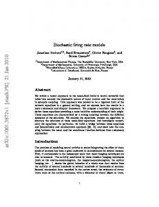
where [x]C ´ x for x > 0 and is zero otherwise; ¯ is the gain parameter. This behavior can be modeled by a Hodgkin-Huxley type single compartment neuron with a slow A-current (Hille, 1984). (See appendix A for the details of the model.) The parameters of the sodium and the potassium currents were chosen to yield a saddle-node bifurcation at the onset of Žring. Figure 1 shows the response of this model neuron without and with the A-current. As can be seen, the A-current linearizes the f-I relationship. Our model neuron has gain value ¯ D 35:4 cm2 /¹Asec.

1812

O. Shriki, D. Hansel, and H. Sompolinsky

120

V [mV]

Firing rate [spikes/sec]

160

50 0 ­ 80 0

100 200 Time [msec]

80 40 0 0

1

2 3 2 I [mA/cm ]

4

5

Figure 1: f-I curves of the single-neuron model with gA D 0 (dashed line), gA D 20 mS=cm2 , ¿A D 0 msec (dash-dotted line), gA D 20 mS=cm2 , ¿A D 20 msec (solid line). Comparison of the three curves shows that linearization of the fI curve is due to the long time constant of the A-current. (Inset) A voltage trace of the single-neuron model with constant current injection of amplitude I D 1:6 ¹A=cm2 for gA D 20 mS=cm2 , ¿A D 20 msec. The neuron’s parameter values are as deŽned in appendix A.

Relatively few experimental data have been published on the dependence of the Žring rate of cortical cells on their leak conductance. However, experimental evidence (Connors, Malenka, & Silva, 1988; Brizzi, Hansel, Meunier, van Vreeswijk, & Zytnicki, 2001) and biophysical models (Kernell, 1968; Holt & Koch, 1997) show that increasing gL affects the f-I curve primarily by increasing its threshold current, whereas its effect on the gain of the curve is weak. We incorporate these properties by assuming that ¯ is independent of gL and that the threshold current increases linearly with the leak conductance, Ic D Ico C Vc gL :

(2.3)

The threshold gain potential Vc measures the rate of increase of the threshold current as the leak conductance, gL , increases, and Ioc is the threshold current when gL D 0. This behavior is also reproduced in our model neuron, as shown in Figure 2. Approximating the f-I curve with equations 2.2 and 2.3 yields Ioc D 0:63 mA=cm2 and Vc D 5:5 mV. This provides a good

Rate Models for Conductance-Based Cortical Neuronal Networks

2 Ic [mA/cm2]

Firing rate [spikes/sec]

160

1813

1.5

120 80

1 0.05

0.1 0.15 2 gL [mS/cm ]

0.2

40 0 0

1

2 3 2 I [mA/cm ]

4

5

Figure 2: f-I curves for gA D 20 mS=cm2 , ¿A D 20 msec, and different values of gL . The curves from left to right correspond to gL D 0:05; 0:1; 0:15; 0:2 mS=cm2 , respectively. (Inset) The threshold current, Ic , as a function of the leak conductance, gL .

approximation of the f-I curve for the range f D 5–150 spikes=sec. For higher Žring rates, the effect of the saturation of the rates becomes signiŽcant and needs to be incorporated into the model. We have found that this effect can be described approximately by an f-I curve of the form f D ¯[I ¡ Ic ]C ¡ ° [I ¡ Ic ]2C ;

(2.4)

with Ic given by equation 2.3. Fitting the Žring rate of our single-neuron model to equation 2.4 yields good Žt over the range f D 5–300 spikes=sec, with the parameter values ¯ D 39:6 cm2 /¹Asec, ° D 0:86 (cm2 /¹A)2 /sec, ® D 6:77 mV, and Ico D 0:59 ¹A=cm2 . The above conductance-based model neuron is the one used in all subsequent numerical analyses. 2.2 Network Dynamics. The network dynamics of N coupled cells are given by

C

dV i D gL .EL ¡ Vi .t// ¡ Iiactive C Iiext C Iinet dt

.i D 1; : : : ; N/;

(2.5)

1814

O. Shriki, D. Hansel, and H. Sompolinsky

where Iinet denotes the synaptic current of the postsynaptic cell i generated by the presynaptic sources within the network. It is modeled as Inet i .t/ D

N X

gij .t/.Ej ¡ Vi .t//;

jD1

(2.6)

where gij .t/ is the synaptic conductance triggered by the action potentials of the presynaptic jth cell and Ej is the reversal potential of the synapse. The synaptic conductance is assumed to consist of a linear sum of contributions from each of the presynaptic action potentials. In our simulations, gij .t/ has the form of an instantaneous jump from 0 to Gij followed by an exponential decay with a synaptic decay time ¿ij , dgij dt

D¡

gij ¿ij

C Gij Rj .t/;

t > 0;

(2.7)

P where Rj .t/ D tj ±.t ¡ tj / is the instantaneous Žring rate of the presynaptic jth neuron and tj are the times of occurrence of its spikes. In general, we deŽne Gij as the peak of gij .t/ and the synaptic time constant as R1 ¿ij D 0 gij .t/ dt=Gij . Synaptic currents from presynaptic sources outside the network are denoted by Iext i . For simplicity, we assume that these sources are all excitatory with the same reversal potential, Einp , peak conductance Ginp , and synaptic time constant, ¿ inp . We assume that these sources Žre Poisson trains of action potentials asynchronously, which generate synaptic conductances with dynamics similar to equation 2.7. Under these assumptions, their summed effects on the postsynaptic neuron i can be represented by a single effective excitatory synapse with peak conductance, Ginp , time constant ¿ inp , and acinp tivated by a single Poisson train of spikes with average rate fi which is the summed rate of all the external sources to the ith neuron. Thus, the external current on neuron i can be written as inp

inp ¡ Vi .t//: Iext i .t/ D gi .t/.E

(2.8)

inp

The quantity gi .t/ satisŽes an equation similar to equation 2.7, inp

dginp gi inp i D ¡ inp C Ginp Ri .t/; dt ¿ inp

t > 0;

(2.9) inp

inp

where Ri is a Poisson spike train with mean rate fi . The value of fi is speciŽed below for each of the concrete models that we study. Due to the inp inp Poisson statistics of Ri , the external conductance, gi .t/, is a random variinp inp able with a time average and variance Ginp fi ¿ inp and .Ginp /2 fi ¿ inp =2,

Rate Models for Conductance-Based Cortical Neuronal Networks

1815

inp

respectively. Note that fi ¿ inp is the mean number of input spikes arriving inp within a single synaptic integration time. The uctuations in Ri constitute the noise in the external input to the network. We deŽne the coefŽcient of variation of thisqnoise as the ratio of its standard deviation and its mean, inp

that is, 1i D 1= 2 fi ¿ inp . As expected, the coefŽcient of variation is proportional to the inverse square root of the total number of spikes arriving within a single synaptic integration time. In particular, one can increase the inp noise level of the input by decreasing fi and increasing Ginp while keeping their product constant. Time-dependent inputs are modeled by a Poisson process with a rate that is modulated in time. In most of the examples studied in this article, we assume a sinusoidal modulation—that the instantaneous Žring rate in the external input to the neuron is inp

f inp .t/ D f0

inp

C f1 cos.!t/;

(2.10)

where !=2¼ is the frequency of the modulation. 2.3 Model of a Hypercolumn in Primary Visual Cortex. We model a hypercolumn in visual cortex by a network consisting of Ne excitatory neurons and Nin inhibitory neurons that are selective to the orientation of the visual stimulus in their common receptive Želd. We impose a ring architecture on the network. The cortical neurons are parameterized by an angle µ, which denotes their preferred orientation (PO). The ith excitatory neuron is parameterized by µi D ¡ ¼2 C i N¼e , and similarly for the inhibitory ones. The peak conductances of the cortical recurrent excitatory and inhibitory synapses decay exponentially with the distance between the interacting neurons, measured by the dissimilarity in their preferred orientations, that is, G® .µ ¡ µ 0 / D

GN ® exp.¡jµ ¡ µ 0 j=¸® /; ¸®

(2.11)

where µ ¡ µ 0 is the difference between the POs of the pre- and postsynaptic neurons. The index ® takes the values e and in. The quantity Ge (resp. Gin ) denotes an excitatory (inhibitory) interaction (targeting either excitatory or inhibitory neurons) with a space constant ¸e (resp. ¸in ). Note that the excitatory as well as the inhibitory interactions are the same for excitatory and inhibitory targets. Additional excitatory neurons provide external input to the network, representing the lateral geniculate nucleus (LGN) input to cortex, each with peak conductance Ginp D GN LGN . The total mean Žring rate of the afferent inputs to a neuron with PO µ is f inp D fLGN .µ ¡ µ0 /, where fLGN .µ ¡ µ0 / D fNLGN C[.1 ¡ ²/ C ² cos.2.µ ¡ µ0 //]:

(2.12)

1816

O. Shriki, D. Hansel, and H. Sompolinsky

The parameter C is the stimulus contrast, and the angle µ0 denotes the orientation of the stimulus. The parameter ² measures the degree of tuning of the LGN input. If ² D 0, the LGN input is untuned: all the neurons receive the same input from the LGN, regardless of their PO and the orientation of the stimulus. If ² D 0:5, the LGN input vanishes for neurons with a PO that is orthogonal to the stimulus orientation. The maximal LGN rate fNLGN is the total Žring rate of the afferents of a stimulus with C D 1 and µ D µ0 . The single-neuron dynamics is given by equation 2.1 and is assumed to be the same for both the excitatory and inhibitory populations. 2.4 Numerical Integration and Analysis of Spike Responses. In the numerical simulations of the conductance-based networks, the nonlinear differential equations of the neuronal dynamics were integrated using a fourth-order Runge-Kutta method (Press, Flannery, Teukolsky, & Vetterling, 1988) with a Žxed time step 1t. Most of the simulations were performed with 1t D 0:05 msec. In order to check the stability and precision of the results, some simulations were also performed with 1t D 0:025 msec. A spike event is counted each time the voltage of a neuron crosses a Žxed threshold value Vth D 0. We measure the instantaneous Žring rate of a single neuron deŽned as the number of spikes in time bins of size 1t D 0:05 msec, averaged over different realizations of the external input noise. We then compute the time average of this response and, in the case of periodically modulated input, the amplitude and phase of its principal temporal harmonic. We also measure the population Žring rate, deŽned as the number of spikes of single neurons in each time bin divided by 1t, averaged over a select population of neurons in the network as well as over the input noise. As in the case of a single neuron, the network response is characterized by the time average and the principal harmonic of the population rate. 3 Rate Equations for General Asynchronous Neuronal Networks The dynamic states of a large network characterized by the above equations can be classiŽed as being synchronous or asynchronous (Ginzburg & Sompolinsky, 1994; Hansel & Sompolinsky, 1996), which differ in terms of the strength of the correlation between the temporal Žring of different neurons. When the external currents, Iiext, are constant in time (except for a possible noisy component which is spatially uncorrelated), the network may exhibit an asynchronous state in which the activities of the neurons are only weakly correlated. Formally, in an asynchronous state, the correlation coefŽcients between the voltages of most of the neuronal pairs approach zero in the limit where the network size, N, grows to inŽnity. Analyzing the asynchronous state in a highly connected network is relatively simple. Because each postsynaptic cell is affected by many uncorrelated synaptic conductances (within a window of its integration time), these

Rate Models for Conductance-Based Cortical Neuronal Networks

1817

conductances can be taken to be time independent. In other words, in the asynchronous state, the spatial summation of the synaptic conductances is equivalent to a time average. Hence, the total synaptic current of each cell can be written as Iinet .t/CIiext .t/ D

N X jD1

inp

Gij ¿ij fj .Ej ¡Vi .t//CGinp ¿ inp fi

.Einp ¡Vi .t//

(3.1)

(see equations 2.6 and 2.8). This current can be decomposed into two components: app

Iinet C Iiext D Ii

C 1IiL :

(3.2)

app

Ii is the component of the synaptic current that has the form of a constant applied voltage-independent current app

Ii

D

N X jD1

inp

Gij ¿ij fj .Ej ¡ EL / C Ginp ¿ inp fi

.Einp ¡ EL /:

(3.3)

The second component of the synaptic current, 1IiL , embodies the voltage dependence of the synaptic current and has the form of a leak current, syn

1ILi D gi .EL ¡ Vi .t//;

(3.4)

where syn

gi

inp

D gnet i C gi

(3.5)

is the mean total synaptic conductance of the ith cell. The quantities gnet i and inp gi are given by gnet i D inp

gi

N X

(3.6)

Gij ¿ij fj ; jD1 inp

D Ginp ¿ inp fi

:

(3.7)

Thus, the discharge of the postsynaptic cell in the asynchronous network can be described by the f-I curve of a single cell with an applied current, equasyn tion 3.3, and a “leak” conductance, which is equal to gL C gi , equation 3.5. Incorporating these contributions in equation 2.2, taking into account the dependence of the threshold current on the total passive conductance as

1818

O. Shriki, D. Hansel, and H. Sompolinsky

given by equation 2.3, yields the following equations for the Žring rates of the cells: app

syn

fi D ¯[Ii ¡ Vc .gL C gi / ¡ Ico ]C " # N X inp D¯ Jij fj C Jinp fi ¡ T ; iD1

C

(3.8) .i D 1; : : : ; N/;

where Jij D Gij ¿ij .Ej ¡ EL ¡ Vc /

(3.9)

and Jinp D Ginp ¿ inp .Einp ¡ EL ¡ Vc /:

(3.10)

The parameter T is the threshold current of the isolated cells, T D Ic .gL /. Note that the subtractive term Vc in equations 3.9 and 3.10 is the result of the increase of the current threshold of the cell due to the synaptic conductance (see equation 2.3). Equation 3.8 is of the form of the self-consistent rate equations that describe the input-output relations for the neurons in a recurrent network at a Žxed-point state. This theory provides a precise mapping between the biophysical parameters of the neurons and synapses and the parameters appearing in the Žxed-point rate equations. The output state variables, given by the right-hand side of equation 3.8, are simply the stationary Žring rates of P inp inp , are the mean synaptic the neurons. The input variables, N fi iD1 Jij fj C J currents at a Žxed potential given by EL C Vc , where Vc is the threshold-gain potential, equation 2.3. Equation 3.9 provides a precise interpretation of the synaptic efŽcacies Jij in terms of the biophysical parameters of the cells and the synaptic conductances. We note in particular that our theory yields a precise criterion for the sign of the efŽcacy of the synaptic connection. According to equation 3.9, synapses with positive efŽcacy obey the inequality Ej > EL C Vc :

(3.11)

Conversely, synapses with negative efŽcacies obey Ej < EL C Vc . The potential EL C Vc is close but not identical to the threshold potential of the cell. Hence, this criterion, which takes into account the dynamics of Žring rates in the network, does not match exactly the biophysical deŽnition of excitatory and inhibitory synapses. The above results allow the prediction not only of the stationary rates of the neurons but also their mean synaptic conductances due to the input from

Rate Models for Conductance-Based Cortical Neuronal Networks

1819

within the network and to the external input. In fact, using equations 3.6 and 3.7 and equations 3.9 and 3.10 yields gnet i D

N X jD1

Jij

fj Ej ¡ EL ¡ Vc

(3.12)

and inp

gi

inp

D Jinp

fi : Einp ¡ EL ¡ Vc

(3.13)

In the following sections, we apply this theory to concrete network architectures. 4 Response of an Excitatory Population to a Time-Independent Input We Žrst test the mapping equations, equations 3.8 through 3.10, in the case of a large, homogeneous network that contains N identical excitatory neurons. The network dynamics are given by equations 2.5 through 2.7 with the single-neuron model of appendix A. Each neuron is connected to all other neurons with a peak synaptic conductance, G, which is the same for all the connections in the network. In addition, each neuron receives a single external synaptic input that has a peak conductance, Ginp , which is activated by a Poisson process with a Žxed uniform rate, f inp . The external synaptic inputs to different cells are uncorrelated. The dynamic response of all synaptic conductances is given by equation 2.7 with a single synaptic time constant ¿e D 5 msec. Applying equations 3.8 through 3.10 to this simple architecture results in the following equation for the mean Žring rate of the neurons in the network, f , f D ¯[Jinp f inp C Jf ¡ Ic ]C

(4.1)

where Jinp D Ginp ¿e .Ee ¡ EL ¡ Vc /

(4.2)

J D NG¿e .Ee ¡ E L ¡ Vc /:

The solution for the Žring rate is f D

¯ [Jinp f inp ¡ Ic ]C : 1 ¡ ¯J

(4.3)

The mean Žring rate, f , of the neurons in the network, as predicted from this equation, is displayed in Figure 3 (dashed line) against the value of the

1820

O. Shriki, D. Hansel, and H. Sompolinsky

250 200 150 100

spikes/sec

Firing rate [spikes/sec]

300 300 200 100 0 0

0.5 1 1.5 2 Input [mA/cm ]

50 0 0

0.02 0.04 0.06 0.08 0.1 2 Synaptic conductance [mS/cm ]

Figure 3: Firing rate versus excitatory synaptic strength in a large network of fully connected excitatory neurons. The rate of the external input is f inp D 1570 spikes=sec, and the synaptic time constant is ¿e D 5 msec. Dashed line: Analytical results from equation 4.3. Solid line: Analytical results when a quadratic Žt is used for the f-I curve, equation 2.4. Circles: Results from simulations of the conductance-based model with N D 1000. (Inset) Firing rate versus external input for strong excitatory feedback (analytical results) showing bistability for NG D 0:49 ¹S=cm2 . The network can be either quiescent or in a stable sustained active state in a range of external inputs, Jinp f inp , less than the threshold current, Ic .

peak conductance of the total excitatory feedback, NG. When the synaptic conductance increases, such that J reaches the critical value J D 1=¯ (corresponding to NG D 0:095 mS=cm2 ), the Žring rate, f , diverges. However, it is expected that when the Žring rate reaches high values, the weak nonlinearity of the f-I curve, given by the quadratic correction, equation 2.4, will need to be taken into account. Indeed, solving the self-consistent equation for f with the quadratic term (solid line in Figure 3) yields Žnite values for f , even when J is larger than 1=¯. In addition, the quadratic nonlinearity predicts that in the high J regime, the network should develop bistability. For a range of subthreshold external inputs, the network can be in either a stable quiescent state or a stable active state with high Žring rates, as shown in the inset of Figure 3. These predictions are in full quantitative agreement with the numerical simulations of the conductance-based excitatory network as shown in Figure 3.

Rate Models for Conductance-Based Cortical Neuronal Networks

1821

5 A Model of a Hypercolumn in Primary Visual Cortex In this section we show how the correspondence between conductancebased models and rate models can be applied to investigate a model of a hypercolumn in V1. When applying the general rate equations, equations 3.8 through 3.10, to the hypercolumn model, we Žrst note that in the asynchronous state, the Žring-rate proŽle of the excitatory and the inhibitory populations is the same. This is because we assume that the interaction proŽles depend solely on the identity (excitatory or inhibitory) of the presynaptic neurons and that the single-neuron properties of the two types of cells are the same. We denote the rate of the (e or in) neurons with PO µ and a stimulus orientation µ0 as f .µ ¡ µ0 /. These rates obey "Z

f .µ ¡ µ0 / D ¯

C¼=2 ¡¼=2

dµ 0 J.µ ¡ µ 0 / f .µ 0 ¡ µ/ ¼ #

C JLGN fLGN .µ ¡ µ0 / ¡ T

;

(5.1)

C

where we replaced the sum over the synaptic recurrent inputs by an integration over the variable µ 0 , which is a valid approximation for a large network. The recurrent interaction proŽle, J.µ /, combines the effect of the excitatory and the inhibitory cortical inputs and has the form J.µ ¡ µ0 / D

X J® exp.¡jµ ¡ µ 0 j=¸® /; ®De;in ¸®

(5.2)

where J® D N® GN ® ¿® .E® ¡E L ¡Vc /, ® D e; in, and JLGN D GN LGN ¿e .Ee ¡EL ¡Vc /; ¿® denotes the excitatory and inhibitory synaptic time constants, and Ne , Nin are the number of neurons in the excitatory and inhibitory populations, respectively. Equations 5.1 and 5.2 correspond to the rate equations 3.8 through 3.10 with the synaptic conductances and input Žring rate, which are given by equations 2.11 and 2.12. In appendix B, we outline the analytical solution of equations 5.1 and 5.2, which allows us to compute the neuronal activity and the synaptic conductances as functions of the model parameters. We used the analytical solution of these rate equations to explore how the spatial pattern of activity of the hypercolumn depends on the parameters of the recurrent interactions (Je ,Jin , ¸e , and ¸in ) and the stimulus properties. 5.1 Emergence of a Ring Attractor. We Žrst consider the case of an untuned LGN input, ² D 0. In this case, equation 5.1 has a trivial solution in which all the neurons respond at the same Žring rate. As shown in

1822

O. Shriki, D. Hansel, and H. Sompolinsky

appendix B, this solution is unstable when the spatial modulation of the effective interaction, equation 5.2, is sufŽciently large. The condition for the onset of this instability is given by equation B.4. When the homogeneous solution is unstable, the system settles into a heterogeneous solution, which has the form f .µ / D M.µ ¡ Ã/. The angle à is arbitrary and reects the fact that the system is spatially invariant. The manifold of stable states that emerges in this system and breaks its spatial symmetry is known as a ring attractor. The function M, which represents the shape of the activity proŽle in each of these states, can be computed analytically, as described in appendix B. Depending on which mode is unstable, the heterogeneous proŽle of activity that emerges consists of a single “hill” of activity or several such “hills.” In appendix B, we describe how the function M can be computed in the case of a state with a single hill. As an example, we consider the case ¸e D 11:5± , ¸in D 43± , and ¯ Jin D 0:73. For this choice of parameters, equation B.4 predicts that the state with a homogeneous response is stable for ¯ Je < 0:87 and unstable for ¯ Je > 0:87. At ¯ Je D 0:87, the unstable mode corresponds to the Žrst Fourier mode. Therefore, the instability at this point should give rise to a heterogeneous response with a unimodal proŽle of activity (a single hill). This is conŽrmed by the numerical solution of the rate equations, 5.1 and 5.2. Using the mapping prescriptions, equation 3.9, these results can be translated into the prediction that if ¸e D 11:5± , ¸in D 43± , Nin GN in D 0:333 mS=cm2 , the homogeneous state is stable for conductance-based model if Ne GN e < 0:138 mS=cm2 , but that it is unstable for Ne Ge > 0:138 mS=cm2 . We tested whether these predictions coincide with the actual behavior of the conductance-based model in numerical simulations. Figures 4A and 4B show raster plots of the network for Ne GN e D 0:133 mS=cm2 and Ne GN e D 0:143 mS=cm2 , respectively. For Ne GN e D 0:133 mS=cm2 , neurons in all the columns responded in a similar way. This corresponds to the homogeneous state of the rate model. Moreover, in this simulation, the average population Žring rate was f D 18 spikes=sec, in excellent agreement with the value predicted from the rate model for the corresponding parameters ( f D 18:05 spikes=sec). In contrast, for Ne GN e D 0:143 mS=cm2 , the network does not respond homogeneously to the stimulus. Instead, a unimodal hill of activity appears. This is congruent with the prediction of the rate model. Since the external input is homogeneous, the location of the peak is arbitrary. In the numerical simulations, the activity proŽle slowly moves due to the noise in the LGN input. The stability analysis of the homogeneous state of the rate model shows that if ¯ Jin > 0:965, which corresponds to Nin GN in D 0:443 mS=cm2 , the mode n D 2 is the one that Žrst becomes unstable when Je increases. This suggests that in this case, the proŽle of activity that emerges through the instability is bimodal. Numerical simulations of the full conductance-based model were found to be in excellent agreement with this expectation (see Figure 5).

Rate Models for Conductance-Based Cortical Neuronal Networks

1823

Preferred orientation [deg]

A

90 60 30 0 ­ 30 ­ 60 ­ 90 0

100

90 60 30 0 ­ 30 ­ 60 ­ 90 0

100

B

200

300

400

500

200

300

400

500

Time [msec]

Figure 4: Symmetry breaking leading to a unimodal activity proŽle. A network with Ne D Nin D 1600 was simulated for two values of the maximal conductance of the excitatory synapses. The external input to the network is homogeneous (² D 0). The input rate is NfLGN D 2700 Hz. The maximal conductance of the input synapses is Ginp D 0:0025 mS=cm2 . Parameters of the interactions are ¸e D 11:5± , N in D 0:333 mS=cm2 . The time constants of the synapses are ¿e D ¸in D 43± , Nin G ¿in D 3 msec. The analytical solution of the rate model equations predicts that for N e < 0:138 mS=cm2 , the response of the network to the input is homogeneous Ne G N e > 0:138 mS=cm2 , it is unimodal. (A) Raster plot of the network and that for Ne G N e D 0:133 mS=cm2 showing that the response is homogeneous. (B) Ne G Ne D for N e G 0:143 mS=cm2 , showing that the response is a unimodal hill of activity. The noise that is present in the system induces a slow random wandering of the hill of activity.

5.2 Tuning of Firing Rates and Synaptic Conductances. We consider now the case of a tuned LGN input, which corresponds to ² > 0. Equation 5.1 shows that in general, the response of a neuron with PO µ depends on the stimulus orientation µ0 through the difference µ ¡µ0 —namely, that f .µ ; µ0 / D M.jµ ¡ µ0 j/. For Žxed µ0 , when µ varies, f .µ ; µ0 / is the proŽle of activity of the network in response to a stimulus of orientation µ0 . Conversely, when µ is Žxed and µ0 varies, f .µ; µ0 / is the tuning curve of the neuron with PO µ. Therefore, the function M determines the tuning curve of the neurons in the model. We now compare the tuning curves of the neurons computed in the framework of the rate model with those in the corresponding simulations

1824

O. Shriki, D. Hansel, and H. Sompolinsky

Preferred orientation [deg]

A

90 60 30 0 ­ 30 ­ 60 ­ 90 0

100

90 60 30 0 ­ 30 ­ 60 ­ 90 0

100

B

200

300

400

500

200

300

400

500

Time [msec]

Figure 5: Symmetry breaking leading to a bimodal activity proŽle. The size of the simulated network is Ne D Nin D 1600. The input rate is NfLGN D 2700 Hz. The maximal conductance of the input synapses is Ginp D 0:0025 mS=cm2 . The parameters of the interactions are ¸e D 11:5± , ¸in D 43± , Nin Gin D 1:33 mS=cm2 . The time constants of the synapses are ¿e D ¿in D 3 msec. The analytical solution N e < 0:196 mS=cm2 , the response of the rate model equations predicts that for Ne G N e > 0:196 mS=cm2 , of the network to the input is homogeneous and that for Ne G N it is bimodal. (A) Raster plot of the network for Ne Ge D 0:19 mS=cm2 , showing that the response is homogeneous. The average Žring rate in the network in the simulation is f D 3:2 spikes=sec, which is in good agreement with the prediction N e D 0:138 mS=cm2 , showing that of the rate model ( f D 2:9 spikes=sec). (B) N e G the response is bimodal. The noise that is present in the system induces a slow random wandering of the pattern of activity.

of the conductance-based network. SpeciŽcally, we take ² D 0:175 and fNLGN D 3400 Hz. For these values, in the absence of recurrent interactions, the response of the neurons to the input exhibits broad tuning. This is shown in Figure 6 (dashed line). The recurrent excitation can sharpen the tuning curves and also amplify the neuron response, as shown in Figure 6. In this Žgure, we plotted the neuronal tuning curve when the parameters of the interactions are ¸e D 6:8± and ¸in D 43± , Ne GN e D 0:125 mS=cm2 , Nin GN in D 0:333 mS=cm2 . The solid line was computed from the solution of the mean-Želd equations of the corresponding rate model. This solution indicates that the tuning width is µC D 30± and that the maximal Žring rate is fmax D 75:5 spikes=sec. The circles are from the numerical simulations of the

Rate Models for Conductance-Based Cortical Neuronal Networks

1825

Firing rate [spikes/sec]

80 60 40 20 0 ­ 90

­ 60

­ 30 0 30 Orientation [deg]

60

90

Figure 6: Tuning curves of the LGN input (dashed line) oriented at µ0 D 0± and the spike response of a neuron with preferred orientation µ D 0± (solid line and circles). The LGN input parameters are ² D 0:175, ginp D 0:0025 mS=cm2 , NfLGN D 3400 Hz. The interaction parameters are ¸e D 6:3± , ¸in D 43± , Ne G Ne D N in D 0:467 mS=cm2 . The time constants of the synapses are 0:125 mS=cm2 , Nin G ¿e D ¿in D 3 msec. The circles are from numerical simulations with Ne D Nin D 1600 neurons. The response of the neuron was averaged over 1 sec of simulation. The solid line was obtained by solving the rate model with the corresponding parameters.

conductance-based model. The agreement with the analytical predictions from the rate model is very good. The input conductances of the neurons in V1 change upon presentation of a visual stimulus. Experimental results (Borg-Graham, Monier, & Fregnac, 1998; Carandini, Anderson, & Ferster, 2000) indicate that with large stimulus contrasts, these changes have typical values of 60% when the stimulus is presented at null orientation, whereas they can be as large as 250 to 300% at optimal orientation. We applied our approach to study the dependence of the total change in input conductance on the space constants of the interactions for a given LGN input. We assume that the cortical circuitry sharpens and ampliŽes the response such that the tuning curves have a given width µC and amplitude fmax . We compute the interaction parameters to achieve tuning curves with a given width, µC and a given maximal discharge rate, fmax . To be speciŽc, we take µC D 30:5± ; fmax D 70 spikes=sec. We also Žxed the space constant of the

O. Shriki, D. Hansel, and H. Sompolinsky

Conductance change [%]

1826

2000 1800 1600 1400 1200 1000 800 600 400 200 0 0

10 20 30 40 Space constant of excitation[deg]

Figure 7: Change in the input conductance in iso (solid line) and crossorientation (dashed line). The lines were computed as explained in the text.

inhibitory interaction, ¸in D 43± , and varied the value of ¸e . For each value of ¸e , we evaluated the values of Je and Jin that yield the desired values of µC and fmax . Subsequently, for each set of parameters, we computed the changes in the input conductance of the neurons, relative to the leak conductance, for a stimulus presented in iso and cross orientation. These changes, denoted by 1giso and 1gcross , respectively, are increasing functions of ¸e , as shown in Figure 7. Actually, it can be shown analytically from the mean Želd equations of the rate model that the conductance changes diverge when ¸e ! ¸in . This is because in that limit, the net interaction is purely excitatory with an amplitude that is above the symmetry-breaking instability. The rate model also allows us to estimate the separate contributions of the LGN input, the recurrent excitation, and the cortical inhibition to the change in total input conductance induced by the LGN input. An example of the tuning curves of these contributions is shown in Figure 8, where they are compared with the results from the simulations of the full model. These results indicate that for the chosen parameters, most of the input conductance contributed by the recurrent interactions comes from the cortical inhibition. This is despite the fact that the spike discharge rate is greatly ampliŽed by the cortical excitation.

Rate Models for Conductance-Based Cortical Neuronal Networks

1827

Conductance change [%]

350 300 250 200 150 100 50 0 ­ 90

­ 60

­ 30 0 30 Orientation [deg]

60

90

Figure 8: Tuning curves of conductances. Solid line: Total change. Dotted line: Contribution to the total change from the LGN input. Dashed line: Contribution to the total change from the recurrent excitatory interactions. Dash-dotted line: Contribution to the total change from the recurrent inhibitory interactions. These lines were obtained from the solution of the mean-Želd equations of the rate model. The parameters are as in Figure 6. The squares, circles, triangles, and diamonds are from numerical simulations. Same parameters as in Figure 6.

6 Rate Response of a Single Neuron to a Time-Dependent Input The analysis of the previous sections focused on situations in which the Žring rates of the neurons were approximately constant in time. We now turn to the question of Žring-rate dynamics, namely, how to describe the neuronal Žring response in the general situation in which the Žring rates are time dependent. We Žrst study the response of a single neuron to a noisy sinusoidal input, equation 2.10. The Žring rate of the neuron (averaged over the noise) can be expanded in a Fourier series: f .t/ D f0 C f1 cos.!t C Á/ C ¢ ¢ ¢ ;

(6.1)

where f0 is the mean Žring rate and f1 and Á are the amplitude and phase of the Žrst harmonic (the Fourier component at the stimulation frequency). Here, we consider only cases in which the modulation of the external input is not overly large, so that there is no rectiŽcation of the Žring rate by the threshold.

1828

O. Shriki, D. Hansel, and H. Sompolinsky

Under these conditions, our simulations show that harmonics with orders higher than 1 are negligible (results not shown). Therefore, the response of the neuron can be characterized by the average Žring rate f0 and the modulation f1 , f1 < f0 . Our simulations also show that the mean response, f0 , depends only weakly on the modulation frequency of the stimulus or on the stimulus amplitude and can be well described by the steady-state frequency-current relation. This is shown in Figure 9 (left panels), where the predictions from the rate model (solid horizontal lines) are compared with the mean output rates in the numerical simulations of the conductancebased model (open circles). Figure 9 also shows the amplitude of the Žrst harmonic of the response and its phase shift Á as a function of the modulation frequency º ´ !=2¼ (Žlled circles). It should be noted that the raw response of the neuron reects two Žltering processes of the external input rate: the low-pass Žltering induced by the synaptic dynamics and the Žltering induced by the intrinsic dynamics of the neuron and its spiking mechanism. To better elucidate the transfer properties of the neuron, we remove the effect of the synaptic lowpass Žltering on the amplitude and phase of the response. (This corresponds p to multiplying f1 by 1 C !2 .¿ inp /2 and subtracting tan¡1 .¡!¿ inp / from the phase.) The results for two values of the mean output rate, f0 ’ 30 spikes=sec and f0 ’ 60 spikes=sec, and for two values of the input noise coefŽcient of inp inp variation, 1 D 0:18 ( f0 D 1125 Hz) and 1 D 0:3 ( f0 D 3125 Hz), are presented. Clearly, both the amplitude and the phase of the response depend on the modulation frequency. Of particular interest is the fact that the amplitude exhibits a resonant behavior for modulation frequencies close to the mean Žring rate of the neuron, f0 . The main effect of increasing the coefŽcient of variation of the noise is to broaden the resonance peak. As in our analysis of the steady-state properties, the external synaptic input can be decomposed here into a current term, and a conductance term, which are now time dependent. The simplest dynamic model would be to assume that the same f-I relation that was found under steady-state conditions, Equations 2.2 and 2.3, holds when the applied current and the passive conductance are time dependent. In our case, this would take the form f .t/ D ¯[I.t/ ¡ .Ico C Vc g.t//]C . This model predicts that the response amplitude does not depend on the modulation frequency and that the phase shift is always zero, in contrast to the behavior of the conductance-based neuron (see Figure 9). To account for the dependence of the modulation frequency, we extend the model by assuming that it has the form f .t/ D ¯[IŽlt.t/ ¡ .Ico C Vc gŽlt.t//];

(6.2)

where IŽlt .t/ and gŽlt .t/ are Žltered versions of the current and conductance terms, respectively. For simplicity, we use the same Žlter for both current and conductance. A Žrst-order linear Žlter can be either a high-pass or a low-pass

Rate Models for Conductance-Based Cortical Neuronal Networks

A

60 40 20 0 60 40 20 0

0 ­ 30 ­ 60 ­ 90

B

Phase [deg]

Amplitude [Hz]

60 40 20 0

C

D

60 40 20 0 0

1829

50

100

0 ­ 30 ­ 60 ­ 90 0 ­ 30 ­ 60 ­ 90 0 ­ 30 ­ 60 ­ 90 0

50

100

Modulation frequency [Hz] Figure 9: Mean, amplitude, and phase of single-neuron rate response as a function of the modulation frequency. The left panels show the mean output rate of the neuron (hollow circles) and the amplitude of the response (Žlled circles). The right panels show the phase of the response. The solid curves are the predictions of the dynamic rate model (see the text). The external input was designed to produce a mean output rate of about » 30 spikes=sec in A and B and » 60 spikes=sec in C and D. A and C show q the responses to inputs with a small noise coefŽcient inp

of variation, 1 D 1= 2 f0 ¿ inp D 0:18, while B and D show the responses to inputs with a high noise level, 1 D 0:3.

Žlter. Since the dependence of the response amplitude on the modulation frequency has a bandpass nature, a Žrst-order linear Žlter would not be suitable. Thus, we assume a second-order linear Žlter. The Žlter for the current is described by 1 d2 IŽlt 1 dIŽlt a dI C C IŽlt D I C ; !0 Q dt !0 dt !20 dt 2

(6.3)

1830

O. Shriki, D. Hansel, and H. Sompolinsky

w0/2p [Hz]

80 60 40 20 0 0

20 40 60 80 Mean output rate [spikes/sec]

Figure 10: Resonance frequency (!0 =2¼ ) as a function of the mean output rate. For each value of the mean output rate, optimal values of !0 were averaged over four noise levels: 1 D 0:15; 0:18; 0:22; 0:3. The range of modulation frequencies for the Žt was 1–100 Hz. The optimal linear Žt (solid line) has a slope of 1 and an offset of 13:1.

and a similar equation (with the same parameters) deŽnes the conductance Žlter. This is the equation of a damped harmonic oscillator with a resonance frequency !0 =2¼ and Q-factor Q (Q is deŽned as !0 over the width at half height of the resonance curve). Note that the driving term is a linear combination of the driving current input and its derivative. We investigated the behavior of the optimal Žlter parameters over a range of mean output rates, 10–70 spikes=sec, and a range of input noise levels, 1 D 0.15–0.3. For lower noise levels, the response proŽle contains additional resonant peaks (both subharmonics and harmonics) that cannot be accounted for by the linear Žlter of equation 6.3. For each mean output rate and input noise level, we ran a set of simulations with modulation frequencies ranging from 1 Hz to 100 Hz, and then numerically found the set of Žlter parameters that gave the best Žt for both amplitude and phase of the response. The variation of the optimal values for Q and a was small under the range of input parameters we considered, with mean values of Q D 0:85 and a D 1:9. The resonance frequency !0 =2¼ depends only weakly on the noise level but increases linearly with the mean output rate of the neuron, with a slope of 1, !0 =2¼ D f0 C 13:1, as shown in Figure 10. The solid curves in Figure 9 show the predictions of equation 6.3 for the amplitude and phase

Rate modulation [spikes/sec]

Rate Models for Conductance-Based Cortical Neuronal Networks

1831

20 10 0 ­ 10 ­ 20 500

1000 1500 Time [msec]

2000

Figure 11: Single-neuron response to a broadband signal. The thick curve shows the rate of the conductance-based neuron, and the thin curve shows the prediction of the rate model. The input consisted of a superposition of 10 cosine functions with random frequencies, amplitudes, and phases (see text for speciŽcs). For clarity, only the uctuations around the mean Žring rate (» 30 spikes=sec) are shown.

of the rate response using the mean values of Q and a and the linear Žt for !0 , mentioned above. The results show that this model is a reasonable approximation of the response modulation of the conductance-based neuron. So far, we have dealt with the Žring-rate response of a single neuron to input composed of a single sinusoid. We also tested the response of the neuron to a general broadband stimulus. For this, we used a Poissonian input characterized by a mean rate and a time-varying envelope that consisted of a superposition of 10 cosine functions with random frequencies, amplitudes, and phases. The mean input rate was chosen to obtain a mean output Žring rate » 30 spikes=sec. The modulation frequencies were drawn from a uniform distribution between 0 and 60 Hz and the phases from a uniform distribution between 0 and 360 ± . The relative amplitudes were drawn from a uniform distribution between 0 and 1, and to avoid rectiŽcation, they were normalized so that their sum is 0:8. The results are presented in Figure 11. They show that the response to a broadband stimulus can be predicted from the response to each of the Fourier components. This conŽrms the validity of our linearity assumption, equation 6.2.

1832

O. Shriki, D. Hansel, and H. Sompolinsky

7 Response of a Neuronal Population to a Time Periodic Input We now apply the approach of the previous section to study the dynamics of a network of interacting neurons in response to a time-dependent input. Here we consider the case of a large, homogeneous network of N fully connected neurons, which receive an external noisy oscillating input. The input to each neuron is a Poisson process with a sinusoidal envelope. In addition, the Žring times of the inputs that converge on different cells in the network are uncorrelated, so that the Poissonian uctuations in the inputs to the different cells are uncorrelated. Nevertheless, since the underlying oscillatory rate of the different inputs is coherent, the network response will have a synchronized component. To construct a simple model of the dynamics of the network rate, we Žrst deŽne two conductance-rate variables, r.t/ D g.t/=.NG¿e / and rinp .t/ D ginp .t/=.Ginp ¿e /, where G and Ginp are the peak conductances of the recurrent and afferent synapses, respectively. Averaging equation 2.7 over all the neurons in the network yields the following equation for the population conductance rate, ¿e

dr D ¡r C f .t/; dt

(7.1)

where f .t/ is the instantaneous Žring rate of the network per neuron. A similar equation holds for rinp .t/, which is a low-pass Žlter of f inp .t/. The equation for f .t/ is f .t/ D ¯[Jinp ½ inp C J½ ¡ Ic ];

(7.2)

where J inp and J are given in equation 4.3. The quantities ½.t/ and ½ inp .t/ are obtained from r.t/ and rinp .t/, respectively, using the Žlter in equation 6.3, 1 d2 ½ !02 dt2

C

1 d½ a dr C½ DrC ; !0 Q dt !0 dt

(7.3)

and a similar equation holds for ½ inp . This yields a set of self-consistent equations, which determine the Žring rate of the neurons in the network, f .t/. For response modulation amplitudes smaller than the mean Žring rate, the dynamics are linear and can be solved analytically (see appendix C). Figure 12 shows the mean, amplitude, and phase of the network response f .t/ obtained by simulating the dynamics of the conductance-based network together with the analytical predictions of the rate model. (As in the previous section, the Žltering done by the input synapses was removed for purposes of presentation.) The mean rate of the Poisson input and the strength of the synaptic interaction were chosen such that the mean Žring rate of the network will be around 50 spikes=sec and the noise level will be 1 D 0:22. The results of Figure 12 reveal the effect of the recurrent interactions on the modulation of the network rate response. Qualitatively, the peak of the

Phase [deg]

Amplitude [Hz]

Rate Models for Conductance-Based Cortical Neuronal Networks

1833

60 40 20 0 0 30

20

40

60

80

100

20 40 60 80 Modulation frequency [Hz]

100

0 ­ 30 ­ 60 ­ 90 0

Figure 12: Response of an excitatory network to a sinusoidal stimulus. (Top) Mean (hollow circles) and amplitude (Žlled circles). (Bottom) Phase. The network consists of N D 4000 neurons. The neurons are coupled all-to-all. The synaptic conductance is NG D 0:039 mS=cm2 , and the synaptic time constant is ¿e D 5 msec. The reversal potential of the synapses was Ve D 0 mV.

response amplitude proŽle is suppressed and shifts to smaller frequencies due to the excitatory connectivity. In contrast, for an inhibitory network, the model predicts that the peak response will be shifted to the right and that the resonant behavior will be more pronounced. This can be proved from equation C.2 by taking negative J. To test this prediction, we ran simulations of a uniform fully connected network with inhibitory synapses (the reversal potential was ¡80 mV). The input parameters and the strength of the synaptic interaction were chosen to produce a mean Žring rate around 50 spikes=sec and a noise level 1 D 0:3. Shown in Figure 13 are the results of the numerical simulations, together with the prediction of the rate model. These results provide additional strong support for our phenomenological time-dependent rate response model. 8 Discussion The rate models derived here are based on speciŽc assumptions about single cell properties. The most important assumptions are the independence of the gain of the f-I curve of the leak conductance, gL (see equation 2.2) and the approximated linear dependence of the threshold current on gL (see

O. Shriki, D. Hansel, and H. Sompolinsky

Phase [deg]

Amplitude [Hz]

1834

60 40 20 0 0 30

20

40

60

80

100

120

20 40 60 80 100 Modulation frequency [Hz]

120

0 ­ 30 ­ 60 ­ 90 0

Figure 13: Response of an inhibitory network to a sinusoidal stimulus. (Top) Mean (hollow circles) and amplitude (Žlled circles). (Bottom) Phase. The network consists of N D 4000 neurons. The neurons are coupled all-to-all. The synaptic conductance is NG D 0:18 mS=cm2 , and the synaptic time constant is ¿e D 5 msec. The reversal potential of the synapses was Vin D ¡80 mV.

equation 2.3). This means that shunting conductances have a subtractive effect rather than a divisive one. This is in agreement with previous modeling studies (Holt & Koch, 1997) and with the properties of the conductancebased model neuron used in our study (see Figure 2). Recent experiments using the dynamic clamp technique provide additional support for this assumption (Brizzi et al., 2001; Chance, Abbott, & Reyes, 2002). A further simplifying assumption, supported by experiments, is that in a broad range of input currents and output Žring rates, the f-I curves of cortical neurons can be well approximated by a threshold linear function. We used such a form of the f-I curve to show that the response of a single neuron to a stationary synaptic input can be well described by simple rate models with threshold nonlinearity. We applied our single-neuron model to the study of a network of neurons, receiving an input generated by a set of synapses activated by uncorrelated trains of spikes with stationary Poisson statistics. In this case, we derived a rate model under the additional assumptions that the network is highly connected and that it is in an asynchronous state. The mapping of the conductance-based model onto a rate model described in this work provides a correspondence between the “synaptic efŽcacy” used in rate models and biophysical parameters of the neurons. In

Rate Models for Conductance-Based Cortical Neuronal Networks

1835

particular, the sign of the synaptic efŽcacy is determined by the value of the reversal potential relative to E L C Vc , where Vc is the threshold gainpotential of the postsynaptic neuron (see equation 2.3). Furthermore, our theory enables the use of rate models to calculate synaptic conductances that are generated by the recurrent activity, allowing a quantitative comparison of predictions from rate models and conductance measurements in in vitro and in vivo intracellular experiments. In the case of a fully connected network of excitatory neurons, we showed that the Žring rate of the neurons predicted by the rate model was highly congruent with simulation results in a broad range of synaptic conductances. This indicates that our rate model provides reliable results over a broad range of Žring rates and conductance changes. Even for very high rates, incorporating a weak quadratic nonlinearity is enough to account for the saturation of the neurons’ Žring rates. We also showed that our approach can be applied to networks with more complicated architectures, such as the conductance-based model of a hypercolumn in V1 analyzed in this work. The conditions for the stabilization of the homogeneous state can be correctly predicted from the mean-Želd analytical solution of the corresponding rate model. Furthermore, the proŽle of activity of the network and the tuning curve of the synaptic conductances can be calculated. Our results show that in order to obtain changes in input conductances that are similar to those found experimentally, one has to assume that the space constant of the excitatory feedback is much smaller than the space constant of the inhibitory interactions. However, this conclusion may depend on our assumption of interaction proŽles, which are identical for excitatory and inhibitory targets. To extend our approach to the case of time-dependent inputs, we studied the response of the single neuron to noisy input that is modulated sinusoidally in time. We showed that this response can be described by a rate model in which the neuron responds instantaneously to an effective input, which is a Žltered version of the actual one. This is similar to the approach of Chance, du Lac, and Abbott (2001), who studied the responses of spiking neurons to oscillating input currents. Our description is valid provided that the input is sufŽciently noisy to broaden resonances and that its modulation is small compared to its average to avoid rate rectiŽcation. Interestingly, if these assumptions are satisŽed, we found that the neuron essentially behaves like a linear device even if the modulation of the input is substantial. This allowed us to derive a rate model that provides a good description for the dynamics of a homogeneous network of neurons receiving a time-dependent input. Our derivation of rate equations for conductance-based models can be compared to the one suggested by Ermentrout (1994; see also Rinzel & Frankel, 1992). Ermentrout derived a rate model in the limit where the synaptic time constants are much longer than the time constants of the currents involved in the generation of spikes, as well as in the interspike

1836

O. Shriki, D. Hansel, and H. Sompolinsky

interval. In this case, the neuronal dynamics on the scale of the synaptic time constants can be reduced to rate equations of the type of equation 7.1 in which the rate variables, r.t/, represent the instantaneous activity of the slow synapses. However, in Ermentrout’s approach, the Žring rate f .t/ is given by an equation similar to equation 7.2 with ½ inp ´ rinp and ½ ´ r. This is in contrast to our approach, where ½ inp and ½ are Žltered versions of rinp and r. The two approaches become equivalent in the limit of slow varying input and slow synapses, that is, !0 À 1=tinp ; 1=¿s where tinp is the typical timescale over which the external input varies and ¿s is the synaptic time constant of the faster synapses in the network. The parameter !0 is the resonance frequency. Knight (1972a, 1972b) studied the response of integrate-and-Žre neurons to periodic input. He concluded that a resonant behavior occurred for input modulation frequencies around the average Žring rate of the neurons. He also showed that white noise in the input broadens the resonance peak. Similar results were obtained by Gerstner (2000) in the framework of spike response models. This resonance has also been reported by Brunel, Chance, Fourcaud, and Abbott (2001) and Fourcaud and Brunel (2002), who studied analytically the Žring response of a single integrate-and-Žre neuron to a periodic input with temporally correlated noise. Our results extend these conclusions to conductance-based neurons. An interesting Žnding of this work is that the resonance frequency of the rate response increases linearly as a function of the mean output rate with a slope of one. It would be interesting to derive this relationship as well as the other parameters of our rate dynamics model from the underlying conductance-based dynamics. In addition, applications of our approach to other single-cell conductancebased models and to more complicated network architectures need to be explored. For instance, the effect of slow potassium adaptation currents should be taken into account. These currents are likely to contribute to the high-pass Žltering of the neuron as shown by Carandini, Fernec, Leonard, and Movshon (1996) in the case of an oscillating injected current. In this work, we used an A-current as a mechanism for the linearization of the f-I curve. Other slow hyperpolarizing conductances might also achieve the same effect (Ermentrout, 1998). In particular, slow potassium currents, which are responsible for spike adaptation in many cortical cells, might be alternative candidates. However, linear f-I curves are also observed in cortical inhibitory cells, most of which do not show spike adaptation, but they probably do possess an A-current. Finally, we focused in this work on conductance-based network models of point neurons. An interesting open question is whether an appropriate rate model can also be derived for neurons with extended morphology. In conclusion, our results open up possibilities for applications of rate models to a range of problems in sensory and motor neuronal circuits in cortex as well as in other structures with similar single-neuron properties. Applying the rate model to a concrete neuronal system requires knowledge of

Rate Models for Conductance-Based Cortical Neuronal Networks

1837

a relatively small number of experimentally measurable parameters that characterize the f-I curves of the neurons in the system. In addition, the rate model requires knowledge of the gross features of the underlying connectivity pattern, as well as an estimate of the order of magnitude of the associated synaptic conductances. Appendix A: Model Neuron This appendix provides the speciŽcs for the equations of the model neuron used here. The dynamics of our single-neuron model consists of the following equations Cm

dV D ¡IL ¡ INa ¡ IK ¡ IA C Iapp: dt

(A.1)

The leak current is given by IL D gL .V ¡ EL /. The sodium and the delayed rectiŽer currents are described in a standard way: INa D gN Na m31 h.V ¡ ENa / for the sodium current and IK D gN K n4 .V ¡ EK / for the delayed rectiŽer current. The gating variables x D h; n satisfy the relaxation equations: dx=dt D .x1 ¡ x/=¿x . The functions x1 , ( x D h; n; m), and ¿x are: x1 D ®x =.®x C ¯x /, and ¿x D Á=.®x C ¯x / where ®m D ¡0:1.V C 30/=.exp.¡0:1.V C 30// ¡ 1/, ¯m D 4 exp.¡.V C 55/=18/, ®h D 0:07 exp.¡.V C 44/=20/, ¯h D 1=.exp.¡0:1.V C 14// C 1/, ®n D ¡0:01.V C 34/=.exp.¡0:1.V C 34// ¡ 1/ and ¯n D 0:125 exp.¡.V C 44/=80/. We have taken: Á D 0:1. The A-current is IA D gN A a31 b.V ¡ EK / with a1 D 1=.exp.¡.V C 50/=20/ C 1/. The function b.t/ satisŽes db=dt D .b1 ¡ b/=¿A with: b1 D 1=.exp..V C 80/=6/ C 1/. For simplicity, the time constant, ¿A , is voltage independent. The other parameters of the model are: Cm D 1¹F=cm2 , gN Na D 100 mS/cm2 , gN K D 40 mS/cm2 . Unless speciŽed otherwise, gL D 0:05 mS/cm2 , gN A D 20 mS/cm2 , and ¿A D 20 msec. The reversal potentials of the ionic and synaptic currents are ENa D 55 mV, EK D ¡80 mV, E L D ¡65 mV, Ee D 0 mV, and Ein D ¡80 mV. The external current is Iapp (in ¹A=cm2 ). Appendix B: Model of a Hypercolumn in V1 : The Mean-Field Equations B.1 The Instability of the Homogeneous State. For a homogeneous input, a trivial solution to the Žxed-point equation, equation 5.1, corresponds to a state in which the responses of all the neurons are the same. However, this homogeneous state can be unstable if the spatial modulation of the interactions is sufŽciently large. The condition for this instability can be derived by solving equation 5.1 in the limit of a weakly heterogeneous input fLGN .µ / as follows. The Fourier expansion of fLGN is fLGN .µ / D

1 X nD1

fn exp.2inµ/;

(B.1)

1838

O. Shriki, D. Hansel, and H. Sompolinsky

where the coefŽcients fn are complex numbers. For weakly heterogeneous inputs, all the coefŽcients but f0 are small. In the parameter regime where the homogeneous state is stable, the response of the network to this input will be weakly heterogeneous. Therefore, the Fourier expansion of the activity proŽle is, m.µ / D

1 X

mn exp.2inµ/;

(B.2)

nD1

where all the coefŽcients but m0 are small. Substituting equations B.1 and B.2 in equation 5.1 and computing the coefŽcients mn , n > 0 perturbatively, one Žnds: mn D

JLGN fn ; 1 ¡ ¯ Jn

(B.3)

where Jn are the Fourier coefŽcients of the interactions. The coefŽcient mn diverges if ¯ Jn D 1. This divergence indicates an instability of the homogeneous state. This instability induces a heterogeneous proŽle of activity with n peaks. The coefŽcients Jn can be computed from equation 5.2. This yields the instability onset condition: Á ! 1¡.¡1/n exp.¡¼=2¸e / 1¡.¡1/n exp.¡¼=2¸in / 2¯ Je CJin D 1: (B.4) 1C4n2 ¸2e 1C4n2 ¸2in B.2 Mean-Field Equations for ProŽle of Activity. We are interested in the case in which the LGN input is broadly tuned, 0 < ² < 1=2, and the effect of the interactions is sufŽciently strong to sharpen substantially the response of the neurons. More speciŽcally, we require that f .µ / D 0 for all the neurons with POs such that jµ ¡ µ0 j > ¼=2. In this case, the solution to equations 5.1 and 5.2 can be found analytically. Taking µ0 D 0, without loss of generality, this solution has the form f .µ / D A0 CA1 cos.¹1 µ/CA2 sin.¹2 µ/CA3 cos.2µ/ f .t/ D 0

for µc < jµj

for jµ j< µc

(B.5) (B.6)

The angle µc is determined by f .§µc / D 0:

(B.7)

Substituting equation B.5 in equation 5.1, one Žnds that ¹ 1 and ¹2 are solutions (real or imaginary) of the equation X ®DE;I

2J® D 1; 1 C ¸2® x2

(B.8)

Rate Models for Conductance-Based Cortical Neuronal Networks

1839

and that the coefŽcients A0 and A3 are given by A0 D A3 D

JNLGN fLGN .1 ¡ ²/ ¡ T 1 ¡ 2Je ¡ 2Jin

JN f ± LGN LGN ²: ¹2 Jin ¹1 Je 1 ¡ 2 1C4¹2 C 1C4¹ 2 1

(B.9) (B.10)

2

Finally, A1 and A2 are obtained from the two equations: F.¸® ; ¹; A/ D 0

® D E; I;

(B.11)

where, ¹ D .¹1 ; ¹2 /, A D .A0 ; A1 ; A2 ; A3 / and F is the function F.x; ¹; A/ D A0 C

X

Ai .cos.¹i µc / ¡ ¹i x sin.¹i µc // 1 C ¹i x 2 iD1;3

(B.12)

with ¹3 D 2 and the angle µc is determined by the condition A0 C A1 cos.¹1 µc / C A2 sin.¹2 µc / C A3 cos.2µc / D 0:

(B.13)

Appendix C: Rate Dynamics in a Neuronal Population with Uniform Connectivity By Fourier transforming equations 7.1, 7.2, and 6.3 (assuming that the Žring rates are always positive), we obtain for ! 6D 0, O fO.!/ D ¯.Jinp ½O inp C J½/;

(C.1)

where ½.!/ O D B.!/Or.!/, rO.!/ D L.!/ fO.!/, ½O inp .!/ D B.!/Orinp .!/, rOinp .!/ D inp O L.!/ f .!/. The low-pass Žlter L.!/ and bandpass Žlter B.!/ are given by L.!/ D 1=1 C i!¿e and B.!/ D .1 C ia!=!0 /=.1 C iw=!0 ¡ ! 2 =!20 /. Putting the above relations in equation C.1 and solving for fO.!/ gives the transfer function of the network, ¯ Jinp B.!/L.!/ Oinp fO.!/ D f .!/; 1 ¡ ¯ JB.!/L.!/

(C.2)

which can be used to predict the time-dependent rate response. Acknowledgments We thank L. Abbott for fruitful discussions and Y. Loewenstein and C. van Vreeswijk for careful reading of the manuscript for this article. This research was partially supported by a grant from the U.S.-Israel Binational Science Foundation and a grant from the Israeli Ministry of Science and the French Ministry of Science and Technology. This research was also supported by the Israel Science Foundation (Center of Excellence Grant-8006/00).

1840

O. Shriki, D. Hansel, and H. Sompolinsky

References Abbott, L. F., & Kepler, T. (1990). Model neurons: From Hodgkin-Huxley to HopŽeld. In L. Garrido (Ed.), Statistical mechanics of neural networks (pp. 5–18). Berlin: Springer-Verlag. Ahmed, B., Anderson, J. C., Douglas, R. J., Martin, K. A., & Whitteridge, D. (1998). Estimates of the net excitatory currents evoked by visual stimulation of identiŽed neurons in cat visual cortex. Cereb. Cortex, 8, 462–476. Amit, D. J. (1989). Modeling brain function. Cambridge: Cambridge University Press. Amit, D. J., & Tsodyks, M. V. (1991). Quantitative study of attractor neural networks retrieving at low spike rates I: Substrate—spikes, rates and neuronal gain. Network, 2, 259–273. Azouz, R., Gray, C. M., Nowak, L. G., & McCormick, D. A. (1997). Physiological properties of inhibitory interneurons in cat striate cortex. Cereb. Cortex, 7, 534–545. Ben-Yishai, R., Lev Bar-Or, R., & Sompolinsky, H. (1995). Theory of orientation tuning in visual cortex. Proc. Natl. Acad. Sci. USA, 92, 3844–3848. Borg-Graham, L. J., Monier, C., & Fregnac, Y. (1998). Visual input evokes transient and strong shunting inhibition in visual cortical neurons. Nature, 393, 369–373. Brizzi, L., Hansel, D., Meunier, C., van Vreeswijk, C., & Zytnicki, D. (2001). Shunting inhibition: A study using in vivo dynamic clamp on cat spinal motoneurons. Society for Neuroscience Abstract, 934.3. Brunel, N., Chance, F. S., Fourcaud, N., & Abbott, L. F. (2001). Effects of synaptic noise and Žltering on the frequency response of spiking neurons. Phys. Rev. Lett., 86, 2186–2189. Carandini, M., Fernec, M., Leonard, C. S., & Movshon, J. A. (1996). Spike train encoding by regular-spiking cells of the visual cortex. J. Neurophysiol., 76, 3425–3441. Carandini, M., Anderson, J., & Ferster, D. (2000). Orientation tuning of input conductance, excitation, and inhibition in cat primary visual cortex. J. Neurophysiol., 84, 909–926. Chance, F. S., du Lac, S., & Abbott, L. F. (2001). An integrate-or-Žre model of spike rate dynamics. Society for Neuroscience Abstract, 821.44. Chance, F. S., Abbott, L. F., & Reyes, A. D. (2002). Gain modulation from background synaptic input. Neuron, 35, 773–782. Churchland, P. S., & Sejnowski, T. J. (1992). The computational brain. Cambridge, MA: MIT Press. Connors, B. W., Malenka, R. C., & Silva, L. R. (1988). Two inhibitory postsynaptic potentials, and GABAA and GABAB receptor-mediated responses in neocortex of rat and cat. J. Physiol. (Lond.), 406, 443–468. Ermentrout, B. (1994). Reduction of conductance based models with slow synapses to neural nets. Neural Comp., 6, 679–695. Ermentrout, B. (1998). Linearization of F-I curves by adaptation. Neural Comp., 10, 1721–1729. Fourcaud, N., & Brunel, B. (2002). Dynamics of the Žring probability of noisy integrate-and-Žre neurons. Neural Comp., 14, 2057–2111.

Rate Models for Conductance-Based Cortical Neuronal Networks

1841

Georgopoulos, A. P., & Lukashin, A. V. (1993). A dynamical neural network model for motor cortical activity during movement: Population coding of movement trajectories. Biol. Cybern., 69, 517–524. Gerstner, W. (2000). Population dynamics of spiking neurons: Fast transients, asynchronous states, and locking. Neural Comp., 12, 43–89. Ginzburg, I., & Sompolinsky, H. (1994). Theory of correlations in stochastic neuronal networks. Phys. Rev. E, 50, 3171–3191. Hansel, D., & Sompolinsky, H. (1996). Chaos and synchrony in a model of a hypercolumn in visual cortex. J. Comput. Neurosci., 3, 7–34. Hansel, D., & Sompolinsky, H. (1998). Modeling feature selectivity in local cortical circuits. In C. Koch & I. Segev (Eds.), Methods in neuronal modeling: From synapses to networks (2nd ed., pp. 499–567). Cambridge, MA: MIT Press. Hille, B. (1984). Ionic channels of excitable membranes. Sunderland, MA: Sinauer. Hodgkin, A. L., & Huxley, A. F. (1952). A quantitative description of membrane current and its application to conduction and excitation in nerve. J. Physiol. (Lond.), 117, 500–562. Holt, G. R., & Koch, C. (1997). Shunting inhibition does not have a divisive effect on Žring rates. Neural Comput., 9, 1001–1013. HopŽeld, J. J. (1984). Neurons with graded response have collective computational properties like those of two-state neurons. Proc. Natl. Acad. Sci. USA, 79, 1554–2558. Kernell, D. (1968). The repetitive impulse discharge of a simple model compared to that of spinal motoneurones. Brain Research, 11, 685–687. Knight, B. W. (1972a). Dynamics of encoding in a population of neurons. J. Gen. Physiol., 59, 734–766. Knight, B. W. (1972b).The relationship between the Žring rate of a single neuron and the level of activity in a population of neurons. Experimental evidence for resonant enhancement in the population response. J. Gen. Physiol., 59, 767–778. Press, W. H., Flannery, B. P., Teukolsky, S. A., & Vetterling, W. T. (1988). Numerical recipes in C: The art of scientiŽc computing. Cambridge: Cambridge University Press. Rinzel, J., & Frankel, P. (1992). Activity patterns of a slow synapse network predicted by explicitly averaging spike dynamics. Neural Comp., 4, 534–545. Rolls, E. T., & Treves, A. (1998). Neural networks and brain function. New York: Oxford University Press. Salinas, E., & Abbott, L. F. (1996). A model of multiplicative neural responses in parietal cortex. Proc. Natl. Acad. Sci. USA, 93, 11956–11961. Seung, H. S. (1996). How the brain keeps the eyes still. Proc. Natl. Acad. Sci. USA, 93, 3339–13344. Stafstrom, C. E., Schwindt, P. C., & Crill, W. E. (1984). Repetitive Žring in layer V neurons from cat neocortex in vitro. J. Neurophysiol., 52, 264–277. Wilson, H. R., & Cowan, J. (1972). Excitatory and inhibitory interactions in localized populations of model neurons. Biophys. J., 12, 1–24. Zhang, K. (1996). Representation of spatial orientation by the intrinsic dynamics of the head-direction cell ensemble: A theory. J. Neurosci., 16, 2112–2126. Received November 14, 2002; accepted January 21, 2003.