Hacettepe Journal of Mathematics and Statistics Volume 36 (2) (2007), 181 – 188
RATIO ESTIMATORS USING ROBUST REGRESSION Cem Kadilar∗, Meral Candan∗ and Hulya Cingi∗
Received 22 : 03 : 2007 : Accepted 22 : 10 : 2007
Abstract We adapt robust regression to ratio-type estimators suggested by Kadilar and Cingi (Ratio estimators in simple random sampling, Applied Mathematics and Computation 151, 893–902, 2004) and obtain the conditions where the adapted estimators are more efficient than the aforementioned estimators in Kadilar and Cingi, in theory. In addition, we support the theoretical results with the aid of a numerical example and simulation having an outlier. Keywords: Ratio estimators, Robust regression, M-estimation, Auxiliary information, Efficiency, Simple random sampling. 2000 AMS Classification: 62 D 05.
1. Introduction Ratio-type estimators take advantage of the correlation between the auxiliary variable, x and the study variable, y. When information is available on the auxiliary variable that is positively correlated with the study variable, the ratio estimator is a suitable estimator to estimate the population mean. For ratio estimators in sampling theory, population information of the auxiliary variable, such as the coefficient of variation or the kurtosis, is often used to increase the efficiency of the estimation for a population mean. However, the outlier problem, which is the present of extreme values in data, generally decreases the efficiency since classical estimators are sensitive to these extreme values [5]. Therefore, in this article, we propose to use Huber M-estimates, instead of least squares (LS) estimates, in ratio estimators in order to reduce the negative effects of outlier data problem. We present traditional ratio estimators for the population mean in simple random sampling and their MSE equations in the next section. We propose ratio estimators and mention their MSE equations in Section 3. Efficiency comparisons between the traditional and the proposed estimators, based on the MSE equations, are considered in Section 4. ∗ Department of Statistics, Hacettepe University, Beytepe 06800, Ankara, Turkiye. E-mail: (C. Kadılar)
[email protected] (M. Candan)
[email protected] (H. Cingi)
[email protected]
182
C. Kadılar, M. Candan, H. C ¸ ıngı
The results of numerical example and simulation are reported in Section 5 and in Section 6, respectively. We arrive at a conclusion from these results in the last section.
2. Traditional Ratio Estimators Motivated by Sisodia and Dwivedi [15], Singh and Kakran [14], and Upadhyaya and Singh [16]; Kadilar and Cingi [10] proposed the following ratio-type estimators (¯ yKC i ; i = 1, 2, ..., 5) for the population mean Y¯ of the study variable y in simple random sampling: ¢ ¡ ¯ −x y¯ + b X ¯ ¯ (2.1) X, y¯KC1 = ¯ ¡x ¢ ¯ −x ¢ y¯ + b X ¯ ¡¯ (2.2) X + Cx , y¯KC2 = x ¯ + Cx ¡ ¢ ¯ −x ¤ y¯ + b X ¯ £¯ y¯KC3 = (2.3) X + β2 (x) , x ¯ + β2 (x) ¡ ¢ ¯ −x ¤ y¯ + b X ¯ £¯ y¯KC4 = Xβ2 (x) + Cx , (2.4) x ¯β2 (x) + Cx ¢ ¡ ¯ −x ¤ ¯ £¯ y¯ + b X (2.5) XCx + β2 (x) , y¯KC5 = x ¯Cx + β2 (x) where Cx and β2 (x) are the population coefficient of variation and the population coefficient of the kurtosis, respectively, of the auxiliary variable; y¯ and x ¯ are the sample means of the study and auxiliary variable, respectively and it is assumed that the population ¯ of the auxiliary variable x is known. Here mean X sxy b= 2 sx
is obtained by the LS method, where s2x and s2y are the sample variances of the auxiliary and the study variable, respectively and sxy is the sample covariance between the auxiliary and the study variable. The MSE equation of the estimators (2.1)–(2.5) can be found using a first degree approximation of the Taylor series expansion, and is as follows: µ 1−f 2 2 2 RKC MSE(¯ yKC i ) ∼ = i Sx + 2BRKC i Sx n (2.6) ¶ + B 2 Sx2 − 2RKC i Sxy − 2BSxy + Sy2 S
(for details see Kadilar and Cingi [10]) where i = 1, 2, . . . 5; B = Sxy 2 is obtained by the x n LS method; f = N ; n is the sample size; N is the population size; Y¯ Y¯ Y¯ , RKC3 = ¯ , RKC1 = R = ¯ , RKC2 = ¯ X X + Cx X + β2 (x) Y¯ β2 (x) Y¯ Cx RKC4 = ¯ and RKC5 = ¯ Xβ2 (x) + Cx X Cx + β2 (x) are the population ratios; Sx2 and Sy2 are the population variances of the auxiliary and study variable, respectively and Sxy is the population covariance between the auxiliary and the study variable. It is worth while pointing out that we take E(b) = B in (2.6) (see [3]), where E represents the expected value. Kadilar and Cingi [10] concluded that all the ratio estimators given above were more efficient than the classical estimators, presented in Sisodia and Dwivedi [15], Singh and
Ratio estimators using robust regression
183
Kakran [14] and Upadhyaya and Singh [16]. This result was obtained with the aid of a numerical example, whose data will also be used in this paper. Note that Kadilar and Cingi [8] adapted these classical estimators for simple random sampling to stratified random sampling, and then Kadilar and Cingi [12] proposed a new ratio estimator that was always more efficient than these adapted estimators in stratified random sampling.
3. Suggested Estimators For the estimation of the population mean, we propose to apply the following 5 ratio estimators using robust regression, instead of ratio estimators presented in (2.1)–(2.5), to data which have outliers: ¢ ¡ ¯ −x ¯ ¯ y¯ + brob X y¯pr1 = (3.1) X, x ¯¡ ¢ ¯ −x ¢ y¯ + brob X ¯ ¡¯ X + Cx , (3.2) y¯pr2 = x ¯ + Cx ¢ ¡ ¯ −x ¤ ¯ £¯ y¯ + brob X y¯pr3 = (3.3) X + β2 (x) , x ¯ + β2 (x) ¡ ¢ ¯ −x ¤ y¯ + brob X ¯ £¯ Xβ2 (x) + Cx , (3.4) y¯pr4 = x ¯β2 (x) + Cx ¡ ¢ ¯ −x ¤ y¯ + brob X ¯ £¯ (3.5) X Cx + β2 (x) , y¯pr5 = x ¯Cx + β2 (x) where brob is obtained by Huber M-estimates in robust regression.
The main advantage of Huber M-estimates over LS estimates is that they are not sensitive to outliers [6]. Thus, when there are outliers in the data, M-estimation is more accurate than LS estimation. Huber M-estimates use a function ρ(e) that is a compromise between e2 and |e|, where e is the error term of the regression model y = a + bx + e, a being the constant of the model. The Huber ρ(e) function has the form: ( e2 −k ≤ e ≤ k, ρ(e) = 2k|e| − k 2 e < −k or k < e, where k is a tuning constant that controls the robustness of the estimator. Huber [7] suggested k = 1.5 σ ˆ , where σ ˆ is an estimate of the standard deviation σ of the population random errors. Details about constant k and M-estimators can be found in Candan [2], Rousseeuw and Leroy [13]. The value of the regression coefficient, brob is obtained by minimizing n X
ρ(yi − a − bxi )
i=1
with respect to a and b [7]. The details for the minimization procedure can be found in Birkes and Dodge [1]. We remark that the MSE equation of the proposed ratio estimators y¯pr i ; i = 1, 2, . . . , 5, is in the same form as the MSE equation in (2.6), but it is clear that B in (2.6) should be replaced by Brob , whose value as obtained by Huber M-estimation is as follows: µ 1−f 2 2 2 MSE (¯ ypr i ) ∼ RKC = i Sx + 2Brob RKC i Sx n (3.6) ¶ 2 + Brob Sx2 − 2RKC i Sxy − 2Brob Sxy + Sy2
184
C. Kadılar, M. Candan, H. C ¸ ıngı
It is well known that since E [Ψ (e)] = 0, where Ψ (e) = ρ0 (e) and e has an identically independent distribution, we can easily assume that E(brob ) = Brob in (3.6), as for b in (2.6). We would like to remark that the value of Brob is computed as brob , but the population data is used for Brob .
4. Efficiency Comparisons In this section we compare the MSE of the proposed estimators, given in (3.6), with the MSE of the ratio estimators, given in (2.6). MSE (¯ ypr i ) < MSE (¯ yKC i ) , i = 1, 2, 3, 4, 5, ¡ ¢ ¡ ¢ 2 2 2Brob RKC i Sx + Brob Sx2 − 2Brob Sxy < 2BRKC i Sx2 + B 2 Sx2 − 2BSxy , ¡ 2 ¢ 2RKC i Sx2 (Brob − B) − 2Sxy (Brob − B) + Sx2 Brob − B 2 < 0, £ ¤ (Brob − B) 2RKC i Sx2 − 2Sxy + Sx2 (Brob + B) < 0.
For Brob − B > 0, that is Brob > B:
2RKC i Sx2 − 2Sxy + Sx2 (Brob + B) < 0, Brob + B < −2RKC i + 2
Sxy , Sx2
Brob < B − 2RKC i . Similarly, for Brob − B < 0, that is Brob < B: Brob > B − 2RKC i Consequently, we have the following conditions: (4.1)
0 < Brob − B < −2RKC i
or (4.2)
−2RKC i < Brob − B < 0.
When condition (4.1) or (4.2) is satisfied, the proposed estimators given in (3.1)–(3.5), are more efficient than the ratio estimator, given in (2.1)–(2.5), respectively.
5. Numerical Illustration We use data in Kadilar and Cingi [10] to compare efficiencies between the traditional and proposed estimators based on the MSE equations. These data concern the level of apple production (in tons) as the study variable and number of apple trees (1 unit =100 trees) as the auxiliary variable in 106 villages of the Aegean Region in Turkey in 1999 (Source: Institute of Statistics, Republic of Turkey). The statistics of the population are given in Table 1. Table 1. Data Statistics Y¯ = 2212.59 ¯ = 274.22 X
RKC1 = 8.0688
ρ = 0.86
Sy = 11551.53
RKC3 = 7.1654
B = 17.21
Sx = 574.61
RKC4 = 8.0670
Brob = 5.02
β2 (x) = 34.57
RKC5 = 7.6109
Syx = 5681761.76
Cx = 2.10
N = 106 n = 30
RKC2 = 8.0076
Ratio estimators using robust regression
185
In Figure 1 we clearly see that there are outliers in the data, so we can expect the proposed estimators to perform better than the traditional estimators. Figure 1. Scatter Graph of Auxiliary and Study Variables. 120000
100000
80000
60000
production
40000
20000
0 0
1000
2000
3000
4000
5000
100 trees Using simple random sampling, we assume a sample size of n=30. We would like to point out that sample size has no direct effect on the efficiency comparisons of the estimators, since the sample size n is not involved in the efficiency conditions (4.1) or (4.2), as shown in Section 4. Note that the correlation, ρ, between the auxiliary and study variable is 0.86 for this data set. We obtain the MSE values of the traditional and proposed estimators as defined in Section 2 and Section 3, respectively, and using these values compute the relative efficiency for each proposed estimator in (3.1)–(3.5) with respect to the traditional estimators in (2.1)–(2.5) using the formulae: (5.1)
RE(¯ ypr i ) =
MSE (¯ ypr i ) ; i = 1, 2, . . . , 5 and j = 1, 2, . . . , 5. MSE (¯ yKC j )
Table 2. Theoretical Results for the Relative Efficiencies of each Proposed Estimator with respect to the Traditional Estimators Relative Efficiencies
y¯KC1
y¯KC2
y¯KC3
y¯KC4
y¯KC5
y¯pr1
0.7217
0.7259
0.7841
0.7219
0.7530
y¯pr2
0.7247
0.7288
0.7873
0.7248
0.7560
y¯pr3
0.7694
0.7738
0.8359
0.7695
0.8027
y¯pr4
0.7218
0.7260
0.7842
0.7219
0.7531
y¯pr5
0.7447
0.7490
0.8090
0.7448
0.7769
186
C. Kadılar, M. Candan, H. C ¸ ıngı
By this way, we compute 25 relative efficiency values for each n, as shown in Table 2 and Table 3. If the relative efficiency value obtained from (5.1) is smaller than 1, then it is apparent that the proposed estimator has a smaller MSE than the estimators presented in Kadilar and Cingi [10]. Therefore, from Table 2, we see that all the proposed ratio estimators are more efficient than the traditional ratio estimators. However, this result is expected because the condition (4.2) is satisfied for all proposed estimators as follows: −2RKC1 ∼ = −2RKC2 ∼ = −2RKC4 ∼ = −16, −2RKC3 ∼ = −15, and = −14 ; −2RKC5 ∼ Brob − B ∼ = −12. Thus, the condition: −2RKC i < Brob − B < 0 is satisfied.
6. Simulation Study The following steps, which were coded in an S-plus program, summarize the simulation ¯ , such as y¯KC i , introduced in procedures used to find the MSE of an estimator, say Yˆ Section 2 or y¯pr i , introduced in Section 3: Step 1: We select 5000 samples of size n from the real data set, mentioned in Section 5, using SRSWOR (simple random sampling without replacement). ¯. Step 2: We use the data from 5000 samples in Step 1 to obtain the value of Yˆ ¯ from 5000 samples for each n. Thus, we find 5000 values of Yˆ ¯ is computed by Step 3: For each n, the MSE of Yˆ 5000 ³ ´ ´2 X³ ¯ = 1 ¯ − Y¯ , MSE Yˆ Yˆ 5000 i=1 where Y¯ is the population mean of the study variable.
In this simulation study, we take sample sizes n = 20, 30, 40, 50. The values of the MSE ratios of the proposed estimators with respect to traditional estimators for each n are given in Table 3. These values are computed using (5.1). From Table 3, we can conclude that all proposed estimators are more efficient than the traditional estimators for all sample sizes. These simulation results support the theoretical findings in Table 2. We would also like to point out that the values of relative efficiencies of the proposed estimators with respect to the traditional estimators in Table 3 would decrease dramatically, in other words, the efficiencies of the proposed estimators would increase significantly, if there were more outliers in data. Table 3. Simulation Results for the Relative Efficiencies of each Proposed Estimator with respect to the Traditional Estimators for various Sample Sizes Sample Sizes
RE (¯ ypr i )
y¯KC1
y¯KC2
y¯KC3
y¯KC4
y¯KC5
n = 20
y¯pr1
0.8799
0.8904
0.9913
0.8802
0.9472
y¯pr2
0.8712
0.8816
0.9815
0.8715
0.9379
y¯pr3
0.8027
0.8124
0.9044
0.8030
0.8642
y¯pr4
0.8796
0.8902
0.9910
0.8799
0.9470
y¯pr5
0.8292
0.8392
0.9342
0.8295
0.8927
Ratio estimators using robust regression
187
Table 3. (Continued) Sample Sizes
RE (¯ ypr i )
y¯KC1
y¯KC2
y¯KC3
y¯KC4
y¯KC5
n = 30
y¯pr1
0.7813
0.7857
0.8184
0.7815
0.8064
y¯pr2
0.7813
0.7856
0.8183
0.7814
0.8063
y¯pr3
0.8029
0.8073
0.8409
0.8030
0.8286
y¯pr4
0.7813
0.7857
0.8184
0.7815
0.8064
y¯pr5
0.7870
0.7914
0.8243
0.7871
0.8122
y¯pr1
0.9446
0.9457
0.9519
0.9447
0.9503
y¯pr2
0.9474
0.9484
0.9546
0.9474
0.9530
y¯pr3
0.9937
0.9948
0.9987
0.9937
0.9976
y¯pr4
0.9447
0.9458
0.9520
0.9448
0.9504
y¯pr5
0.9671
0.9682
0.9745
0.9672
0.9729
y¯pr1
0.9021
0.9025
0.9042
0.9021
0.9043
y¯pr2
0.9048
0.9053
0.9069
0.9049
0.9070
y¯pr3
0.9481
0.9485
0.9503
0.9481
0.9503
y¯pr4
0.9022
0.9026
0.9043
0.9022
0.9044
y¯pr5
0.9239
0.9243
0.9260
0.9239
0.9261
n = 40
n = 50
7. Conclusion From the theoretical discussion in Section 4, and the results of the numerical example and simulation, we infer that the proposed estimators are more efficient than the ratio estimators in Kadilar and Cingi [10] when there are outliers in data. This article shows that M estimation can be used for the ratio estimators of the population mean in simple random sampling and that using M estimation improves the efficiency of ratio estimators. Chambers [4] produced the same result for M estimation in the regression estimator. In forthcoming studies, we hope to adapt the method presented here to estimators using two auxiliary variables as suggested by Kadilar and Cingi [9, 11].
References [1] Birkes, D. and Dodge, Y. Alternative Methods of Regression (John Wiley & Sons, 1993). [2] Candan, M. Robust Estimators in Linear Regression Analysis (Hacettepe University, Department of Statistics, Master Thesis (in Turkish), 1995). [3] Cochran, W. G. Sampling Techniques (John Wiley and Sons, New-York, 1977). [4] Chambers R. L. Outlier robust finite population estimation, Journal of the American Statistical Association 81, 1063–1069, 1986. [5] Chatterjee, S. and Price, B. Regression Analysis by Example, (Wiley, Second Edition, 1991). [6] Hampel, F. R., Ronchetti, E. M., Rousseeww, P. J. and Stahel, W. A. Robust Statistics (John Wiley & Sons, 1986). [7] Huber, P. Robust Statistics (Wiley, New York, 1981). [8] Kadilar, C. and Cingi, H. Ratio estimators in stratified random sampling, Biometrical Journal 45, 218–225, 2003. [9] Kadilar, C. and Cingi, H. Estimator of a population mean using two auxiliary variables in simple random sampling, International Mathematical Journal 5, 357–360, 2003.
188
C. Kadılar, M. Candan, H. C ¸ ıngı
[10] Kadilar, C. and Cingi, H. Ratio estimators in simple random sampling, Applied Mathematics and Computation 151, 893–902, 2004. [11] Kadilar, C. and Cingi, H. A new estimator using two auxiliary variable, Applied Mathematics and Computation 162, 901–908, 2005. [12] Kadilar, C. and Cingi, H. A new ratio estimator in stratified random sampling, Communications in Statistics: Theory and Methods 34, 597–602, 2005. [13] Rousseeuw, P. and Leroy, A. Robust Regression and Outlier Detection, (Wiley, New York, 1987). [14] Singh, H. P. and Kakran, M. S. A modified ratio estimator using known coefficient of kurtosis of an auxiliary character, unpublished, 1993. [15] Sisodia, B. V. S. and Dwivedi, V. K. A modified ratio estimator using coefficient of variation of auxiliary variable, Journal of Indian Society Agricultural Statistics 33, 13–18, 1981. [16] Upadhyaya, L. N. and Singh, H. P. Use of transformed auxiliary variable in estimating the finite population mean, Biometrical Journal 41, 627–636, 1999.