Ray Tracing Tools for High Frequency Electromagnetics ... - CiteSeerX

Ray Tracing Tools for High Frequency Electromagnetics Simulations Sandy Sefi

Stockholm 2003 Licentiate Thesis Royal Institute of Technology Department of Numerical Analysis and Computer Science

Akademisk avhandling som med tillst˚ and av Kungl. Tekniska Högskolan framlägges till offentlig granskning för avl¨ aggande av teknisk licentiatexamen torsdagen den 12 juni 2003 kl 14.15 i sal E33, Kungl. Tekniska Högskolan, Lindstedtsvägen 3, Stockholm. ISBN 91-7283-545-1 TRITA-NA-0314 ISSN 0348-2952 ISRN KTH/NA/R-03/14-SE c Sandy Sefi, May 2003 ° Universitetsservice US AB, Stockholm 2003

Abstract Keywords: CEM, GTD, Ray Tracing, NURBS, Software Design, Shadowing. Over the past 20 years, the development in Computational Electromagnetics has produced a vast choice of methods based on the large number of existing mathematical formulations of the Maxwell equations. None of them dominate over the others, instead they complement each other and the choice of method depends on the frequency range of the electromagnetic waves. This work is focused on the most popular method in the high frequency scenario, namely the Geometrical Theory of Diffraction (GTD). The main advantage of GTD is the ability to predict the electromagnetic field asymptotically in the limit of vanishing wavelength, when other methods, such as the Method of Moments, become computationally too expensive. The low cost of GTD is due to both the fact that there is no runtime penalty in increasing the frequency and that the ray tracing, which GTD is based on, is a geometrical technique. The complexity is then no longer dependent on electrical size of the problem but instead on geometrical sub problems which are manageable. For industrial applications the geometrical structures, with which the rays interact, are modelled by trimmed Non-Uniform Rational B-Spline (NURBS) surfaces, the most recent standard used to represent complex free-form geometries. Due to the introduction of NURBS, the geometrical sub problems tend to be mathematically and numerically cumbersome, but they can be highly simplified by proper Object Oriented programming techniques. This allowed us to create a flexible software package, MIRA: Modular Implementation of Ray Tracing for Antenna Applications, with an architecture that separates mathematical algorithms from their implementation details and modelling. In addition, its design supports hybridisation techniques in combination with other methods such as Method of Moment (MoM) and Physical Optics (PO). In a first hybrid application, a triangle-based PO solver uses the shadowing information calculated with the ray tracer part of MIRA. The occlusion is performed between triangles and their facing NURBS surfaces rather than between their facing triangles, thus reducing the complexity. Then the shadowing information is used in an iterative MoM-PO process in order to cover higher frequencies, where the contribution of the shadowing effects, in the hybrid formulation, is believed to be more significant. Thesis presented at the Royal Institute of Technology of Stockholm in 2003, for the degree of Licentiate in Scientific Computing.

ISBN 91-7283-545-1 • TRITA-NA-0314 • ISSN 0348-2952 • ISRN KTH/NA/R-03/14-SE

iii

iv

Acknowledgements The work described in this thesis has been carried out from November 1999 to April 2003 at the Department of Numerical Analysis and Computer Science (NADA), at the Royal Institute of Technology (KTH). During these years, it has been a true privilege to work at NADA. For this, I am grateful to my supervisor Prof. Jesper Oppelstrup whom I thank for his time, his constant encouragement and for always enlighting the positive side of a situation. I am also grateful to Dr. Bo Strand for an efficient project leading as well as for his directions. Furthermore I would like to mention my colleague Stefan Hagdahl and former colleague Prof. Fredrik Bergholm for their friendship and their efforts in building MIRA. I would also like to thank Maryline Bruel, Lennart Hellström, Dr. Anders Nilsson, Ulf Oreborn, Olga Syrowattchenko and Dr. Anders ˚ Alund for their various contributions and hard work in MIRA. In addition, I wish to thank Jonas Hamberg, Anders Jensen, Erik Söderstr¨ om ˚ and Hans-Johan Asander (Saab Avionics AB) for participation in the beta tests and interesting and professional feedback. All the complex aircraft geometries have been borrowed from them. The text was reviewed by Prof. Jesper Oppelstrup, Prof. Fredrik Bergholm for the ray tracing part, Dr. Anders ˚ Alund for the shadowing and Dr. Ulf Andersson for the parallelisation part. Last, I thank Prof. Patrick Chenin (LMC-IMAG) and Dr. Francois-Regis Degott (UNIVAL S.A.) from my former University Joseph Fourier, Grenoble, France, for pushing me further and for providing access to their research as well as comparative benchmark results. Financial support has been provided by NADA, KTH, PSCI and the National Aeronautical Research Program (NFFP) within the GEMS and SMART projects.

v

vi

Contents 1 INTRODUCTION TO CEM 1.1 Review of the CEM Methods . . . . . . 1.1.1 Exact Numerical Methods . . . . 1.1.2 Approximate Numerical Methods 1.2 Background: PSCI research projects . . 1.2.1 GEMS Project: 1998-2000 . . . . 1.2.2 SMART Project: 2001-2003 . . . 1.3 Thesis Overview and Division of Work . 1.4 The Geometrical Theory of Diffraction . 1.4.1 Historic . . . . . . . . . . . . . . 1.4.2 Advantages of GTD . . . . . . . 1.4.3 Limitations of GTD . . . . . . .

. . . . . . . . . . .

. . . . . . . . . . .

. . . . . . . . . . .

. . . . . . . . . . .

. . . . . . . . . . .

. . . . . . . . . . .

. . . . . . . . . . .

. . . . . . . . . . .

. . . . . . . . . . .

. . . . . . . . . . .

. . . . . . . . . . .

. . . . . . . . . . .

. . . . . . . . . . .

. . . . . . . . . . .

. . . . . . . . . . .

1 1 2 2 3 4 5 5 7 7 9 10

2 GEOMETRICAL MODELLING 2.1 Common Geometric Models . . . . . . . . . 2.2 Constraints and Properties of the B-Rep . . 2.3 Parametric Domain of Definition . . . . . . 2.4 Non-Rational Bezier Curves and Surfaces . 2.4.1 Non-Rational Bezier Curves . . . . . 2.4.2 Non-Rational Bezier Surfaces . . . . 2.5 Rational Bezier Curves and Surfaces . . . . 2.6 Non-Uniform Rational B-Spline (NURBS) . 2.7 Transformation B-Spline to Rational Bezier

. . . . . . . . .

. . . . . . . . .

. . . . . . . . .

. . . . . . . . .

. . . . . . . . .

. . . . . . . . .

. . . . . . . . .

. . . . . . . . .

. . . . . . . . .

. . . . . . . . .

. . . . . . . . .

. . . . . . . . .

. . . . . . . . .

. . . . . . . . .

11 12 13 15 15 16 17 17 18 19

. . . . . . . .

21 21 24 24 28 29 32 32 33

. . . . . . . . . . .

3 RAY TRACING PRINCIPLES 3.1 General Idea . . . . . . . . . . . . . . . . . . . 3.2 Ray-Surface Intersection . . . . . . . . . . . . . 3.2.1 Related Work . . . . . . . . . . . . . . . 3.2.2 Conversion to a Minimisation Problem . 3.2.3 Pre-processing Steps . . . . . . . . . . . 3.2.4 Starting Candidates for the Iteration . . 3.2.5 The CG Iteration . . . . . . . . . . . . . 3.2.6 Inside or Outside the Trimming Curves vii

. . . . . . . .

. . . . . . . .

. . . . . . . .

. . . . . . . .

. . . . . . . .

. . . . . . . .

. . . . . . . .

. . . . . . . .

. . . . . . . .

. . . . . . . .

. . . . . . . .

viii

Contents 3.3

3.4

3.5

3.6

3.7

3.8

Direct Propagation Model . . . . . . . . . . . . . . . . 3.3.1 Direct Rays . . . . . . . . . . . . . . . . . . . . 3.3.2 Incident Field . . . . . . . . . . . . . . . . . . . 3.3.3 Direct Field . . . . . . . . . . . . . . . . . . . . Transmission Through Thin Absorbing Layers . . . . . 3.4.1 Transmitted Rays . . . . . . . . . . . . . . . . 3.4.2 Transmitted Field . . . . . . . . . . . . . . . . Reflection Model . . . . . . . . . . . . . . . . . . . . . 3.5.1 Near to Near Analysis . . . . . . . . . . . . . . 3.5.2 Near to Far Analysis . . . . . . . . . . . . . . . 3.5.3 Mono-static Far to Far . . . . . . . . . . . . . . 3.5.4 Reflected Field . . . . . . . . . . . . . . . . . . Diffraction Model . . . . . . . . . . . . . . . . . . . . . 3.6.1 Geometric Representation of the Curves . . . . 3.6.2 Minimisation in Near to Far Analysis . . . . . 3.6.3 Minimisation in Near to Near Analysis . . . . . Creeping Waves Model . . . . . . . . . . . . . . . . . . 3.7.1 Shadow Line Cast by the Source on the Surface 3.7.2 Geodesic Curve on a Parametric Surface . . . . 3.7.3 Crossing Over Surfaces . . . . . . . . . . . . . . 3.7.4 Shadow Line Cast by the Receiver . . . . . . . Multiple Interactions Model . . . . . . . . . . . . . . . 3.8.1 Double Diffraction . . . . . . . . . . . . . . . . 3.8.2 Double Reflection . . . . . . . . . . . . . . . . 3.8.3 Diffraction Reflection . . . . . . . . . . . . . . 3.8.4 Reflection Diffraction . . . . . . . . . . . . . .

. . . . . . . . . . . . . . . . . . . . . . . . . .

. . . . . . . . . . . . . . . . . . . . . . . . . .

. . . . . . . . . . . . . . . . . . . . . . . . . .

4 SOFTWARE DESIGN AND ARCHITECTURE 4.1 Design considerations . . . . . . . . . . . . . . . . . . . . . 4.1.1 General Constraints . . . . . . . . . . . . . . . . . . 4.1.2 Goals . . . . . . . . . . . . . . . . . . . . . . . . . . 4.2 Architectural Strategies . . . . . . . . . . . . . . . . . . . . 4.2.1 Reuse of Existing Software Components . . . . . . . 4.2.2 Hybridisations . . . . . . . . . . . . . . . . . . . . . 4.2.3 Modularity and Object Orientation . . . . . . . . . . 4.2.4 Modern Programming Style . . . . . . . . . . . . . . 4.2.5 Accuracy and Flexibility . . . . . . . . . . . . . . . . 4.2.6 Handling of Complex Models, Memory Requirements 4.2.7 Robustness . . . . . . . . . . . . . . . . . . . . . . . 4.3 System Architecture . . . . . . . . . . . . . . . . . . . . . . 4.3.1 Overview of the Main Architecture . . . . . . . . . . 4.3.2 Geometry Package . . . . . . . . . . . . . . . . . . . 4.3.3 Ray Package . . . . . . . . . . . . . . . . . . . . . . 4.3.4 Antenna Application Package . . . . . . . . . . . . .

. . . . . . . . . . . . . . . . . . . . . . . . . . . . . . . . . . . . . . . . . .

. . . . . . . . . . . . . . . . . . . . . . . . . . . . . . . . . . . . . . . . . .

. . . . . . . . . . . . . . . . . . . . . . . . . . . . . . . . . . . . . . . . . .

. . . . . . . . . . . . . . . . . . . . . . . . . . . . . . . . . . . . . . . . . .

. . . . . . . . . . . . . . . . . . . . . . . . . .

34 34 35 35 36 36 37 38 38 39 40 40 41 41 43 43 44 45 45 48 48 49 49 50 51 52

. . . . . . . . . . . . . . . .

53 53 53 53 55 55 56 56 56 57 57 57 57 57 58 61 68

Contents

ix

4.4

68

Performance and Benchmark . . . . . . . . . . . . . . . . . . . . . .

5 SHADOWING BASED ON RAY TRACING 5.1 Background . . . . . . . . . . . . . . . . . . . . . . . . . 5.2 Related Work . . . . . . . . . . . . . . . . . . . . . . . . 5.2.1 Shadowing in Facets Based Software . . . . . . . 5.2.2 Shadowing in Parametric Surface Based Software 5.2.3 Triangles on Parametric Surfaces . . . . . . . . . 5.3 Ray Tracing Implementation in MIRANDA . . . . . . . 5.4 Results on a Plate and a Sphere . . . . . . . . . . . . . 5.5 Results on a Grounded Cylinder . . . . . . . . . . . . . 5.6 Parallel Implementation Using MPI . . . . . . . . . . . 5.6.1 Parallel Strategy . . . . . . . . . . . . . . . . . . 5.6.2 Parallelisation Implementation . . . . . . . . . . 5.6.3 Results, Timing and Performance . . . . . . . . . 6 CONCLUSION AND FUTURE WORK

. . . . . . . . . . . .

. . . . . . . . . . . .

. . . . . . . . . . . .

. . . . . . . . . . . .

. . . . . . . . . . . .

. . . . . . . . . . . .

. . . . . . . . . . . .

75 75 76 76 78 78 79 81 84 87 87 88 89 91

x

List of Figures 1.1 1.2 1.3 1.4

Common Entities of Electromagnetics Problems. . . . . . Numerical Methods for the Maxwell Equations. . . . . . . GEMS Hybrid Software Suite for the Maxwell Equations. The Rays of GTD. . . . . . . . . . . . . . . . . . . . . . .

. . . .

2 3 4 8

2.1

Trimming Curves Cutting out a Surface. . . . . . . . . . . . . . . . .

15

3.1 3.2 3.3 3.4 3.5 3.6 3.7 3.8 3.9 3.10 3.11 3.12 3.13 3.14 3.15 3.16

Three Possible Configurations for a Ray. . . . . . . . . . . . . . . . . Distance Ray-Surface in Near to Far Configuration. . . . . . . . . . . Slab Method for Ray/Bounding Boxes Intersection. . . . . . . . . . . Sample Points and Sample Normals. . . . . . . . . . . . . . . . . . . Possible Configurations for the Trimming Curves. . . . . . . . . . . . Direct Propagation in Near to Near Analysis. . . . . . . . . . . . . . Principal Radii of Curvature of the Wavefront in Free Space. . . . . Near to Near Reflect-Transmitted Rays on a Plate in Front of a Cube. Reflection on a Trimmed Surface in the Near to Near Case. . . . . . Diffraction on a Curve in the Near to Near Analysis. . . . . . . . . . Trimming Curve Internal Representation for a Cylinder. . . . . . . . Example of the Creeping Rays on a Cylinder. . . . . . . . . . . . . . Geodesics on a Sphere in Near to Near Configuration. . . . . . . . . Double Diffraction in Near to Near. . . . . . . . . . . . . . . . . . . . Double Reflection on Two Facing Surfaces in Near to Near. . . . . . Diffraction Reflection in Near to Near. . . . . . . . . . . . . . . . . .

22 28 30 31 34 35 36 37 38 41 42 44 46 49 51 52

4.1 4.2 4.3 4.4 4.5 4.6 4.7 4.8 4.9 4.10 4.11

Features of MIRA’s Architecture. . . . . . . . . . . . . . MIRA’s Architecture Decomposed into Three Packages. List of the Geometry Modules. . . . . . . . . . . . . . . Hierarchical Geometry Data Structure. . . . . . . . . . . List of the Ray Modules. . . . . . . . . . . . . . . . . . . Ray’s Internal Data Structure Implementation. . . . . . Event’s Internal Data Structure Implementation. . . . . Direct Propagation Algorithm Implementation. . . . . . Reflection Algorithm Implementation. . . . . . . . . . . Diffraction Algorithm Implementation. . . . . . . . . . . Reflection on a Cone . . . . . . . . . . . . . . . . . . . .

54 58 59 60 62 63 64 65 65 66 66

xi

. . . . . . . . . . .

. . . .

. . . . . . . . . . .

. . . .

. . . . . . . . . . .

. . . .

. . . . . . . . . . .

. . . .

. . . . . . . . . . .

. . . .

. . . . . . . . . . .

. . . . . . . . . . .

xii

List of Figures 4.12 4.13 4.14 4.15 4.16 4.17 4.18 4.19

Min-Max Diffraction on a Cone . . . . . . List of the Antenna Application Modules. FASANT versus MIRA for Diffraction. . . FASANT versus MIRA for Direct. . . . . FASANT versus MIRA for Reflection. . . Direct and Reflection on a Space Station. Gripen-like Aircraft, Top View. . . . . . . Gripen-like Aircraft, Side View. . . . . . .

. . . . . . . .

. . . . . . . .

. . . . . . . .

. . . . . . . .

. . . . . . . .

. . . . . . . .

. . . . . . . .

. . . . . . . .

. . . . . . . .

. . . . . . . .

. . . . . . . .

. . . . . . . .

. . . . . . . .

. . . . . . . .

. . . . . . . .

67 68 69 70 70 71 72 72

5.1 5.2 5.3 5.4 5.5 5.6 5.7 5.8 5.9 5.10 5.11

Shadowing Approaches in Existing PO Solvers. Plate-Sphere Test Case, the Geometry. . . . . . Plate-Sphere Test Case, Measurement. . . . . . Plate-Sphere Test Case, Calculations. . . . . . Grounded Cylinder Test Case, the Geometry. . Grounded Cylinder Test Case, Calculations. . . PO Surface Current on an Aircraft. . . . . . . . Shadowing on an Aircraft. . . . . . . . . . . . . Flowchart of the Parallelisation Process. . . . . Vampir Global Timing Graph for 8 Processors. Total Execution Time on Several Processors. .

. . . . . . . . . . .

. . . . . . . . . . .

. . . . . . . . . . .

. . . . . . . . . . .

. . . . . . . . . . .

. . . . . . . . . . .

. . . . . . . . . . .

. . . . . . . . . . .

. . . . . . . . . . .

. . . . . . . . . . .

. . . . . . . . . . .

. . . . . . . . . . .

77 81 82 83 85 85 86 86 87 89 90

Chapter 1

INTRODUCTION TO CEM Electromagnetics is the scientific discipline that treats electric and magnetic sources as well as the fields these sources produce in specified environments. Computational electromagnetics (CEM) may be defined as the branch of electromagnetics that involves the use of computers in order to obtain numerical results. The CEM, thanks to the past 20 years of development, now represents a third tool that has been added to the two classical tools of experimental observation and mathematical analysis. CEM is applied in growing industrial applications such as the computation of mobile phone coverage, or antenna design and radar stealth technologies for aircraft. Typically, CEM simulations assist the analysis of installed antenna performance or of Radar Cross Section (RCS). Such simulations are conducted to replace expensive and time consuming measurements especially in design and manufacturing stages of the product life-cycle. Their aim is to predict, as realistically as possible, the field scattered, or radiated, by conducting structures, e.g., buildings, aircraft, satellites, cars or ships, or to predict the field emitted by antennas installed on the mentioned objects in order to reduce electromagnetic disturbances or to optimise performance. While a variety of specialised electromagnetic problems can be identified, a very common ingredient, see Figure 1.1, is to establish a relationship between a cause -the incident waves or the sources- and its effect -the response at some receiver location. The mathematical form used to describe these relationships will characterise the specifics of the computational method. Over the past years, the development in CEM has produced a vast choice of methods due to the large number of existing mathematical formulations. None of them dominate over one another, they all have pros and cons and complement each other. In the following, some of the more popular ones are listed.

1.1

Review of the CEM Methods

The Maxwell equations, see [Jackson 98], provide the starting point for the study of all electromagnetic problems. There are two main groups of numerical methods 1

2

Chapter 1. INTRODUCTION TO CEM

Figure 1.1. Common Entities of Electromagnetics Problems.

for the Maxwell equations, the exact and the approximate methods.

1.1.1

Exact Numerical Methods

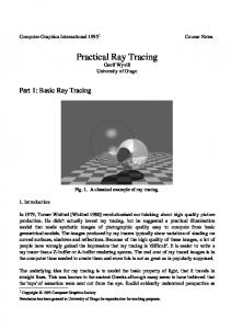
The principal rigorous methods are the Volume Methods, for instance Finite Element Time Domain (FETD) [Rao 82], see Figure 1.2 (a), which express the Maxwell equations by a variational formulation over the entire volume studied, containing both the objects as well as the free space around them. Then come the local Volume Methods, such as Finite Difference Time Domain (FDTD) [Taflove 95], see Figure 1.2 (b), which express the Maxwell equations locally over a volume decomposed into cells. Finally, the Boundary Methods, for example the Method of Moment (MoM) [Harri 68], see Figure 1.2 (c), are deduced from the vector wave equations equivalent to the Maxwell equations. Exact methods have a computational complexity that grows with frequency like f n , where f is the frequency and are also limited by memory size. For instance, MoM complexity with direct solution has n = 6.

1.1.2

Approximate Numerical Methods

For high frequencies, the rigorous numerical methods become unrealistic tools due to computational demand increasing with the frequency. Approximations to the Maxwell equations can be employed to evaluate the electromagnetic field, see [Kouyo 65]. In such context, the problem is formulated in terms of diffraction of an electromagnetic wave by an obstacle. The key point of the classification of the approximate methods is the electrical size of the problem. The electrical size is defined as the ratio between the dimension of the obstacles D, and the wavelength λ = c/f , where c is the speed of light: • When D ¿ λ, the fields are quasi-transverse electromagnetic and the Maxwell equations are approximated by a static solution. • When D À λ, one can use asymptotic methods based on Fermat’s principle and on ray tracing techniques, such as Geometrical Optics (GO) and Geometrical Theory of Diffraction (GTD) [Keller 62], Figure 1.2 (d).

1.2. Background: PSCI research projects

3

• When D ∼ λ, rigorous solutions are necessary. In most complex configurations the three cases above can occur simultaneously. In such conditions, a rigorous formulation is used alone with a substantial computational cost, or hybridised together with approximate methods.

Figure 1.2. Numerical Methods for the Maxwell Equations.

1.2

Background: PSCI research projects

The research and development described in this work was conducted during two projects, GEMS (General Electro Magnetic Solvers) and SMART (Signature Modelling and Reduction Tools), within the Parallel and Scientific Computing Institute, PSCI. PSCI was created in 1995 as one of the 28 VINNOVA competence centers in Sweden. A competence center is a consortium between academy and industry, with the goal to enhance concentration and stimulate academic research in which industrial companies participate actively in order to achieve long term benefits. In this context, the research program meets the industrial needs and the theoretical developments suitable for PhD thesis work by joining application experts from the industrial partners together with graduate students, post-docs and senior scientists.

4


1.2.1

GEMS Project: 1998-2000

A pioneer project in state-of-the-art CEM, GEMS stands for General Electro Magnetic Solvers. It was a Swedish three-year code development project supported by a PSCI research program and co-funded by the National Aeronautical Research Program (NFFP). The industrial partners involved were Ericsson Microwave System, Saab Ericsson Space and Saab Avionics. The academic partners were the Royal Institute of Technology, Uppsala University, the Swedish Institute of Applied Mathematics and the Swedish Defense Research Agency. The academic partners were responsible for research and code development whereas the industrial partners were responsible for specifications, post and preprocessing, and validation of the software. Each partner contributed to the funding, which made GEMS the largest CEM project ever realized in Sweden.

Figure 1.3. GEMS Hybrid Software Suite for the Maxwell Equations.

The main objective of GEMS was to develop a software suite for the Maxwell equations that will be used in an industrial environment. The core of the software is two hybrid codes, one for the time domain and one for the frequency domain, see Figure 1.3: • The time-domain code is hybrid between FDTD [Andersson 01], explicit FVTD and implicit FETD [Edelvik 02], where each method can also be used on its own. Also, a thin-wire sub-cell model have been introduced to the FDTD method [Ledfelt 01]. • The frequency-domain code is hybrid between MoM, PO [Edlund 01], GO and GTD, where each method can also be used on its own. A multilevel

1.3. Thesis Overview and Division of Work

5

Fast Multi-pole Method (FMM) [Nilsson 02] has been developed to boost the performance of the MoM. All codes are mainly written in the Fortran 90 programming language. The parallelisation is performed using MPI [1] and OpenMP [2]. The version control system CVS [3] is used to keep track of the changes. We use the netCDF [4] format for output data which allows visualisation in Matlab [5] and OpenDX [6]. The hybrid meshes, structured and unstructured grids are generated by the CAD software CADfix [7] which is also used to create the geometries and to import IGES [8] or STEP [9] files. A more detailed description of the GEMS software suite can be found in [PSCI 99].

1.2.2

SMART Project: 2001-2003

The SMART (Signature Modelling and Reduction Tools) project is one branch of the continuation of GEMS with application focus on radar signature of aircraft and of Unmanned Aerial Vehicles (UAV). It is aimed to develop a state-of-the-art software suite for RCS applications, in order to compute and optimise the RCS performance of future low radar signature vehicles. It is supported by NFFP and involves KTH, Uppsala University, and Chalmers Universities as academic partners and Saab Avionics as industrial.

1.3

Thesis Overview and Division of Work

This thesis is focused on the development of the high frequency software suite, from its early design stage in GEMS up to the present and future extensions in SMART. The structure of the thesis is decomposed into the following chapters: • Chapter 1: Geometrical Theory of Diffraction. In the second part of this chapter, GTD is introduced based on Geometric Optics and Diffraction theory. It assumes that all waves are ”well-formed” and are locally plane. This enables the use of ray tracing algorithms with the following advantages: + Ray tracing is not memory intensive in comparison to other electromagnetics methods. + Ray tracing is geometric. The computational demand depends on the geometric nature of the structures and not on their electrical size. • Chapter 2: Geometrical Modelling used for High Frequency Calculations. Chapter 2 describes the CAD geometry used as input for the software. GTD assumes all the structures are electrically large and smooth. Such structures are modelled by trimmed NURBS (Non-Uniform Rational B-spline) and rational Bezier surfaces. NURBS is a CAD standard for parametric surface representation.

6

Chapter 1. INTRODUCTION TO CEM • Chapter 3: Ray Tracing Model for Electromagnetics Simulations. Chapter 3 presents the method used for the ray tracing. The solver takes into account the different following effects: Direct Incident, Reflected, Diffracted, Double Reflected, Reflected-Diffracted, and Creeping Waves. All these rays have paths determined by a generalisation of Fermat’s principle. • Chapter 4: Software Design and Architecture Considerations. Chapter 4 describes the Object Oriented design and how it has been developed with the idea to remain general enough in order to support future hybridisation techniques combined with other CEM methods. • Chapter 5: Ray Tracing Shadowing for Iterative MoM-PO Hybrid Solver. In Chapter 5, some hybrid experiments are described. One of our first hybrid applications uses the ray tracer as a stand-alone solver coupled with an iterative MoM-PO solver in order to determine accurately the shadow regions of the PO domain when it is illuminated by a plan wave or an MoM antenna. Several shadowing techniques have been investigated and they are described in the sections that follow.

The ideas found in Chapter 2 have been first formulated in [Chenin 98] then further developed in [Chenin 99]. The material in Chapter 3 concerning the ray propagation models have been inspired by [Catedra 98]. It is given mainly as mathematical background information. Chapter 4 and Chapter 5 are partially based on the following papers: (a) Fredrik Bergholm, Stefan Hagdahl, Sandy Sefi, “Modular approach to GTD”, Proceedings of AP2000, Davos, Switzerland, April 2000. (b) Sandy Sefi, “MIRA: Design and Architecture, a Ray-based Electromagnetics Code”. Thesis for the“Diplôme de Recherches Technologiques” (DRT), University Joseph Fourier, Grenoble, France, October 2000. (c) Sandy Sefi, “Architecture and Geometrical Algorithms in MIRA”, Proceedings of EMB01, Uppsala, Sweden, November 2001. The authors of MIRA are Fredrik Bergholm, Stefan Hagdahl and myself. MIRA is based on the FASANT software, a Fortran 77 code developed at Cantabria University, Spain, by F. Catedra and co-workers [Perez 99]. FASANT did not satisfy all of our requirements (see section 4.1) and therefore we decided to redesign it using the modular Fortran 90 language (see sections 4.2 and 4.3). Fredrik Bergholm specified the input-output for the Geometry Package described in section 4.3.2, co-designed with me the geometric data structures and then, implemented it with Lennart Hellström. He also introduced better diffraction algorithms which use the topological relationships between surfaces and curves discussed in section 3.6.1, and with me, implemented the “Inside material” algorithm described in section 3.2.6.

1.4. The Geometrical Theory of Diffraction

7

Stefan Hagdahl specified the input-output for the field computations, co-designed with me the Antenna Application Package (see 4.3.4) and re-implemented the field calculations with the help of Ulf Oreborn. I am responsible for the main software architecture (see 4.3.1) as well as for the Ray Package. I elaborated its design as described in section 4.3.3, and then reimplemented it. Olga Syrowattchenko helped with the creeping rays (see 3.7) and Maryline Bruel with the transmitted rays (see 3.4). I carried out most of the bug tracking for the software in its totality on different computer architectures such as SUN, SGI or IBM. Finally, I elaborated, implemented and parallelised an innovative shadowing algorithm based on ray tracing on parametric NURBS surfaces for an iterative MoM-PO hybrid solver. All the tested realistic aircraft geometries have been borrowed from Saab Avionics and Figure 5.7 was produced by Erik Söderstr¨ om using the PO solver at Saab Avionics. The results in the section 5.4 were obtained with the assistance of Anders ˚ Alund and finally, Figure 5.6 was produced by Bo Strand using the shadowing algorithm plugged into the MoM-PO solver at Saab Avionics.

1.4

The Geometrical Theory of Diffraction

The Geometrical Theory of Diffraction (GTD) is an asymptotic method for the solution of the Maxwell equations. A thorough description can be found in [Kouyo 65], but the details are beyond the scope of this thesis. We are going to pass through the theory that was originally developed by Keller and his associates in 1962 at the Courant Institute of Mathematical Sciences and since then has dominated the high frequency scenario.

1.4.1

Historic

[Keller 62] showed how the diffraction phenomena, associated with the presence of geometrical discontinuities, may be included in the high frequency solution, as an extension of Geometrical Optics, the oldest and most widely used theory of light propagation. In fact, GO does not specify what happens when a ray hits edges or vertices, which is the creation of diffracted rays. In particular, Keller observed that high frequency diffraction, like reflection and transmission, is a local phenomenon. The field, at a given point of observation, does not depend on the field in all the points on the surface of the obstacle, but only on the field in the neighbourhood of some points on the object, called diffraction points. In doing so, he reduced the complex scattering of electromagnetic waves from arbitrary surfaces to a superposition of simple canonical problems. A summary of the historical process of the diffraction propagation phenomenon can be found in [Bucci 94]. The scattering phenomenon is then divided into two more or less distinct parts: I. A global interaction and combination of the scattered field contributions from different diffraction points of the surface, including calculations of light propagation paths (shadowing).

8

Chapter 1. INTRODUCTION TO CEM II. A local problem of how the incident and scattered fields are related at a particular point on the surface.

Figure 1.4. The Rays of GTD.

As a consequence, the signal reaching a receiver is superposed from a finite number of different propagation paths, that can be determined independently. In GTD, the considered wave propagation phenomena are the incident direct illumination, reflection, diffraction by edges or tips, and surface diffraction waves also known as creeping waves. These phenomena will be called effects in the following, and all together form the ray tracer. The ray tracing consists in drawing (“tracing”) all the propagation paths between a fixed source and a receiver. In Figure 1.4, given the source location, the surrounding area will be divided into four regions: • The perfectly electric conducting (PEC) structure, which no ray can penetrate. • Region III, where only the diffraction, generated at the diffraction point Qe , will contribute to the field at the receiver location. No direct illumination reaches this region since the PEC occludes the direct ray. • Region II, where the direct illumination will be added to the field at any observer location in this region. • Region I, where the field will be increased with the reflection generated from the point R. Note that when another structure is added to the scene, the picture gets more complicated and a shadowing analysis must be performed for all the rays in order to determine whether or not they are occluded.

1.4. The Geometrical Theory of Diffraction

1.4.2

9

Advantages of GTD

The main advantage of GTD is its ability to predict the electromagnetic field asymptotically in the limit of vanishing wavelength, when methods such as the MoM become computationally too expensive. The low computational cost depends on both the fact that there is no run-time penalty in increasing the frequency, as well as the benefits from the ray tracing. First, ray tracing is geometric. The computational demand depends on geometrical features with length scales on the order of the wavelength and not on the electrical size of the problem. The complexity is reduced to geometrical sub problems which are doable. The geometrical sub problems also tend to be mathematically and numerically cumbersome. In fact, searching for relevant ”flash points” in a complex 3-D environment or the analysis of inter visibility, shadowing and multiple scattering are not at all straightforward. But this can be managed, and highly simplified, by computer science methodology combined with Object Oriented programming technology. That allows the creation of a software architecture that separates mathematical modelling from the implementation details. More details about the software organisation and architecture are presented later in Chapter 4. Second, ray tracing algorithms are relatively easy to parallelise both on supercomputers and clusters of workstations. Finally, GTD gives physical insight into the high frequency scattering process in terms of rays emanating from isolated flash points. In fact, ray tracing leads to a very attractive picture of rays on the structure. In many cases this can help engineers to better understand the diffractions or to control the reflections from a structure. Below six of the main advantages of GTD are summarised: + Frequency independent. GTD will give results at higher frequencies when other methods cannot + Electrical size independent. Suitable for large structures such as aircraft or boats. + Low computational cost. Fast execution time compared to rigorous numerical methods. + Low memory requirements. No huge matrix to store. + Easily parallelised. Efficient on supercomputers. + Informative. GTD gives physical insights of the high frequency phenomena. Also, GTD is a wide spread technique in electromagnetics but can be applied to other scientific areas. For instance, including diffraction phenomena has been studied in Acoustics and Mechanics. In Virtual Acoustics, [Tsingos 01] uses diffraction

10


to model realistic reverberant sound in 3D virtual worlds. In Applied Mechanics, [Persson 93] uses the diffraction coefficients to treat elastic wave scattering by cracks.

1.4.3

Limitations of GTD

Despite the nice features summarised before, GTD has a few drawbacks which may sometimes reduce the usefulness of the results. First, GTD is approximate in nature. The accuracy of the calculated field is relatively low since the theory will only yield the leading terms in the asymptotic high frequency solution of the Maxwell equations. Second, GTD is only applicable to electrically large structures. This means that the theory is valid when the wavelength is small compared to the size of the obstacles. Thus it cannot model small details on board of a large structure. Third, GTD is not valid inside boundary layers, i.e., narrow regions in which equation solutions change rapidly. For instance, transition regions between the illuminated region and shadow zone are excluded. In such regions, the GO fields fall non physically abruptly to zero. There exist refined methods to overcome this problem, for example the Uniform Theory of Diffraction (UTD) which adapt the diffraction coefficients to such cases, see [Kouyoumjian 84]. In Figure 1.4, the dashed lines around Region II represent the transition lines where GTD is not valid. Finally, the diffracted fields become infinite inside the caustics, i.e., the envelop of the rays, since the waves are no longer ”well-formed” in such regions. Therefore, in this work we assume the receivers and the sources to be placed outside of any transition regions or caustics.

Chapter 2

GEOMETRICAL MODELLING This chapter gives a description of the geometry supported by MIRA. The concept of geometric models and the functions for handling geometry are commonly used in many branches of computer sciences: • Computer-Aided Design (CAD) CAD-designers model geometric objects, say a piston engine or a model aircraft, with CAD tools (e.g., CADfix, AutoCAD, Pro-Engineer, Catia or Euclid). These programs use free-formed surfaces represented by Bezier, Tensor Product and NURBS basis functions. • Computational Geometry Computational geometers study the algorithmic aspects and complexity measure of geometric problems involving simple geometric objects. Some classical problems are: (a) Computing the convex hull of a set of points. (b) Intersection detection. (c) Triangulate a polygon. Typical efficient algorithms frequently use methods like Divide and Conquer, Recursion and Dynamic Programming. Geometric algorithms involve the manipulation of objects which are not handled at the machine language level. Therefore these complex objects must be organised in larger data structures like Sets, Sequences, Trees or Doubly-Connected-Edge-Lists. • Computer Graphics 11

12

Chapter 2. GEOMETRICAL MODELLING Wherever graphics is involved, geometric objects appear. A good example of visualisation is medical scanning. An object is scanned producing many contours on parallel planes. Then the scanned object is reconstructed, including its interior, from the given contours. • Computer Vision In computer vision and image processing, features are extracted from images. For example, two cameras are mounted on a robot to take stereo pictures. Features are extracted and give feedback to algorithms which control the motion of the robot so it will not collide with the surrounding environment. • Computational Physics In light modelling, computational electromagnetics or acoustics, physicists try to capture, as realistically as possible, the behaviour of waves interacting with complex geometric objects. Their aim is to better understand the characteristics of these phenomena.

In all these mentioned domains, an important consideration is the type of object representation and its associated database structure. There are a number of different representations for an object, such as polygonal flat facets, or implicit or parametric surfaces, with different levels of complexity. The more complex a representation, the more realistic the results it produces, and the longer the simulation takes. Therefore when choosing a representation, a compromise must be reached between realism and efficiency. According to the requirements of CEM applications, a complex representation based on parametric surfaces has been chosen in this work. The following part gives an overview of the most commonly used 3-D geometric models as well as some arguments about our specific choice.

2.1

Common Geometric Models

There are three main classes of common geometric models: 1. Constructive Solid Geometry Representation (CSG) CSG with implicit surfaces, essentially uses Boolean set operations (e.g., set union, intersection and difference), constructors or grammatical rules applied on closed primitives in 3-D space. Thus, a CSG solid can be written as a set equation and can be considered as a design methodology. CSG models provide easy object definition which is very intuitive especially when the solids are relatively simple and show symmetries. The data storage for primitive geometries is efficient [Muuss 99]. However two main drawbacks appear: - CSG is not flexible: the applicability of the CSG depends on the primitive set. If an inappropriate set of primitives is offered, object modelling will become difficult.

2.2. Constraints and Properties of the B-Rep

13

- CSG lacks boundary information of importance especially for visualisation, which requires the triangulation of the boundaries of the solid to be rendered. In our case, boundary information is needed for the representation and localisation of the edges of the solid. 2. Boundary Representation with Facets: The surfaces of 3-D objects can be divided into discrete, flat triangles. Once the surfaces have been triangulated, the 3-D objects may actually be described as a list of elements of the triangulation. Realistic models can be obtained by conversions into triangles of a CAD model. However, while triangulation offers what appear to be precise techniques, behind the scenes they are inherently inaccurate and must be tolerance dependent. To illustrate this, one can think about the difference between reflections from a disco ball and a smooth sphere. The triangles must be extremely small to accurately describe the model. 3. Boundary Representation with Parametric Surfaces: The 3-D objects involved are defined by a list of surface boundaries, the geometric information, and the links between these surfaces, the topological information. Boundary models offer a very flexible tool for modelling man-made objects and are widely used in the vehicle industries (car, aircraft, boat). In fact they allow descriptions of the surfaces for the dies which form the sheets for the wings of the aircraft or the doors of the car. So, it becomes tempting to be able to build software for simulation on the very same geometry which permits the creation of the real shape, see [Suratteau 98], [Degott 99]. In the following, the geometric objects and their manipulation are described. A boundary representation with parametric 3-D surfaces will be used. The surfaces will be trimmed by 2-D curves in their parametric domain of definition. This allows immediate localisation of the edges.

2.2

Constraints and Properties of the B-Rep

Boundary representations are based on a surface-oriented view of solid objects and make explicit the boundary of the object, i.e., the set of points from which any neighbourhood intersects both the ”inside” and the ”outside” of the object. Practically, the “digital” object is a layered description of a real object. The first layer contains zero-dimensional entities, the vertices, the second layer one-dimensional entities, the edges, the third layer two-dimensional entities, the surfaces, the object itself being a three-dimensional entity, a solid. The study of these ”boundary entities” of n-D belongs to the domain of the curves and surfaces, see [Chenin 99]. In order to simplify the manipulation and the development of algorithms working on the object, it is useful to establish, in the internal data structures, some links between the ”boundary entities”. This is called the topological information (in the algebraic topological sense). In this way, an object is characterised by, see [Chenin 98]:

14

Chapter 2. GEOMETRICAL MODELLING

(a) Geometric information: nature of the geometric entities. The solid consists of a set of surfaces and the geometric information usually consists of equations of the edges and surfaces. Surfaces can be flat polygons, Bezier surfaces or NURBS surfaces. Each surface is bordered by a set of edges that can be segments, Bezier curves or NURBS curves, and so on. (b) Topological information: links between the 3-D, 2-D, 1-D and 0-D surfaces. In addition to connectivity, topological information also includes orientation of edges and surfaces. There is no way to go up from a n-D entity to (n + 1)-D entities, but some n-D entities may share (n − 1)-D entities. In this way, neighbour entities in the topological sense are implicitly obtained through access routines. The definition of these neighbourhoods is generally constrained by the orientation of the entities from one to another, so that, see [Chenin 99]: 1. The bordering edges have to be ordered to form a closed curve (a loop). In order to separate the ”inside” of a solid object from its ”outside”, the neighbour edge list associated to each surface has to be ordered. 2. Edges have neighbouring surfaces intersecting at the edge. 3. Edges are limited by neighbouring vertices. There is a need for describing the common part of the border between two surfaces. The vertices of the corresponding edges of the two surfaces must be the same. 4. Vertices have a set of neighbouring edges which intersect at them. 5. The ordering of the vertices that surround a given surface must guarantee that the normal vector to this surface is pointing to the exterior of the solid. Commonly, the order is counter clockwise. If this surface is given by an equation, the equation must be written so that the normal vector points to the exterior of the solid. Therefore, by inspecting normal vectors one can immediately tell the inside/outside of a solid. This orientation must be done for all the surfaces. In addition, the geometric model has to fulfil the following conditions: + The set of surfaces forms a complete skin to the solid with no missing parts + Surfaces do not intersect each other except at common vertices or edges. + The boundaries of surfaces do not intersect themselves. These conditions disallow self-intersecting and open objects. + Surfaces are homeomorphisms, i.e., one to one mappings of sets in parametric 2D-spaces. This avoids degenerated surfaces.

2.4. Non-Rational Bezier Curves and Surfaces

2.3

15

Parametric Domain of Definition

Parametric curves or surfaces, defined in all points of the parametric space Ω, are intervals [a, b] of R (for the curves) or [a, b] × [c, d] of R2 (for the surfaces). Parametric trimming curves are curves inside which or outside which the physical material is located. They have their own definition (one speaks then of natural curve or surface of R3 ) but the re-parameterisation has to be associated with the geometric object, see [Chenin 99]: (a) For a curve, it will be an interval included in the initial Ω. (b) For a surface, it will be a set of curves of R2 (parametric space) that bound (trim) the domain of definition Ω, Figure 2.1. Note here that in presence of holes or of several related components, the orientation and the parameterisation of the trimming curves must be consistent. When following a curve, one should find the ”material” on the left. The material may either be removed inside or outside the trimming curves.

Figure 2.1. Trimming Curves Cutting out a Surface.

2.4

Non-Rational Bezier Curves and Surfaces

MIRA handles trimmed Non-Rational B-Spline (NURBS) surfaces by converting them into rational Bezier patches. In this part, some basic facts of parametric B-spline, Bezier and Bernstein bases are defined. More detailed discussions and practical guides can be found in [Farin 88] where the polynomials are expressed in a particular basis, the Bernstein basis, and some geometric properties becomes apparent.

16

Chapter 2. GEOMETRICAL MODELLING The Bernstein polynomials of degree n are defined for all integers n 6= 0 by: Bin (t) =

n! ti (1 − t)n−i i!(n − i)!

(2.1)

where t ∈ [0, 1] and for mathematical convenience Bin (t) = 0 if i ∈ / {0, 1, ..., n}. The properties of the Bernstein Basis are: • {Bin }i∈{0,1,...,n} forms a basis for the vector space of polynomials of degree less than or equal to n: polynomials can be added together, can be multiplied by a scalar, and all the vector space properties hold. • The Bernstein polynomials form a partition of unity:

Pn

n i=0 Bi (t)

=1

• Recursive definition of the Bernstein polynomials Bin (t) = (1 − t)Bin−1 (t) + n−1 tBi−1 (t) allows stable numerical evaluation. • Bernstein polynomials are all non-negative: 0 ≤ Bin (t) ≤ 1 n (1 − t) • Bin (t) = Bn−i i+1 n n • Degree raising: Bin−1 (t) = n−i n Bi (t) + n Bi+1 (t). Any of the lower-degree Bernstein polynomials (degree < n) can be expressed as a linear combination of Bernstein polynomials of degree n.

• Derivatives of Bernstein polynomials of degree n can be expressed as linear n−1 d n Bi (t) = n(Bi−1 combination of polynomials of degree n − 1: dt (t) − Bin−1 (t))

2.4.1

Non-Rational Bezier Curves

A non-rational Bezier curve [Bezier 74] is defined by the Bernstein basis: t ∈ [0, 1] → C(t) =

n X

Pi Bin (t) ∈ Rm

(2.2)

i=0

The polygonal line {Pi }i∈{0,...,n} is called the control polygon associated to the Bezier curve C. The points Pi are called Control points of the Bezier curve. Bezier curves have various properties which help predict the change in curve produced by a change in the control points. Among these there are: • The curve passes through the start and end points P0 and Pn of the control polygon. • Since the Bezier basis functions are non-zero almost everywhere, changing a control point Pi changes the shape of the curve everywhere. This is the non-localness property. • The tangent to the curve at t = 0 lies in the direction of the line joining the first point to the second point. Also the tangent to the curve at t = 1 is in the direction of the line joining the penultimate point to the last point.

2.5. Rational Bezier Curves and Surfaces

17

• Any point on the curve lies inside the convex hull of the control polygon. Also moving a control point will drag the curve in the same direction. • It can also be proved that any line/plane intersects the curve no more times than it intersects the control polygon. This is called the Variation Diminishing Property. • The degree of the curve is related to the number of control points. Hence using many control points to control the curve shape means evaluating high degree polynomials. • The curve is transformed by applying any affine transformation to its control points and generating the transformed curve from the transformed control points.

2.4.2

Non-Rational Bezier Surfaces

One can extend the definition of curves to the case of surfaces. A parametric Bezier surface, defined by tensor product, is a polynomial application defined in [0, 1]2 with values in R3 , represented in the Bernstein basis by: (u, v) ∈ [0, 1]2 → S(u, v) =

n X m X

Pij Bin (u)Bjm (v)

(2.3)

i=0 j=0

The properties of the Bezier curves apply also to the non-rational Bezier surface in the corresponding way: • The surface does not in general pass through the control points except for the corners of the control point grid. • The surface is contained within the convex hull of the control polygon. • Along the edges of the control grid, the Bezier surface matches the Bezier curve through the control points along that edge.

2.5

Rational Bezier Curves and Surfaces

Rational Bezier curves are expressed in the following way: Pn αi Pi Bin (t) t ∈ [0, 1] → C(t) = Pi=0 n n i=0 αi Bi

(t)

(2.4)

where Pi are the control points in Rm thus C(t) has values in Rm . Each control point Pi has an associated weight αi . The weights αi are real and, in general, chosen positive in order to assure the stability of the numerical algorithms.

18

Chapter 2. GEOMETRICAL MODELLING Rational Bezier surfaces are defined by: Pn 2

(u, v) ∈ [0, 1] → S(u, v) =

Pm n m i=0 j=0 αij Pij Bi (u)Bj (v) Pn Pm n m i=0 j=0 αij Bi (u)Bj (v)

(2.5)

Rational Bezier curves are useful for curve design and representation, but they require high degrees to represent complex shapes thus potentially introducing oscillation and computational cost. To overcome these disadvantages, one can use composite Bezier curves also called “Splines” [DeBoor 78]. A set of Bezier curves joined under certain continuity conditions constitute a B-Spline curve. The B-Spline curves overcome the disadvantages of the simple (non-composite) Bezier curves, that is, complex curves can be modelled with low-degree curves and they admit the local control property. Due to their flexibility, today, B-Splines basis are the most widely used tool in the CAD systems. Moreover, the simple Bezier can be considered as a particular case of B-Spline.

2.6

Non-Uniform Rational B-Spline (NURBS)

NURBS are generalisations of non-rational B-splines, rational and non-rational Bezier curves and surfaces. NURBS curves are a vector-valued piecewise rational polynomial functions of the form [Piegl 91]: Pn αi Pi Nip (t) t ∈ [0, 1] → C(t) = Pi=0 p n i=0 αi Ni

(t)

(2.6)

where αi are the weights, the Pi are the control points (just as in the case of nonrational curves), and Nip (t) are the normalised B-spline basis functions of degree p defined recursively as: (

Ni0 (t)

Nip (t) =

=

1 if ti ≤ t ≤ ti+1 0 otherwise

)

ti+p+1 − t t − ti Nip−1 (t) + N p−1 (t) ti+p − ti ti+p+1 − ti+1 i+1

(2.7)

(2.8)

where ti are the so-called knots forming a knot vector T = {t0 , t1 , , tm }. The degree, number of knots, and number of control points are related by the formula m = n + p + 1. For non-uniform B-splines, the knot vector takes the form: T = {0, 0, 0, , tp+1 , , tm−p−1 , 1, 1, , 1} where 0 and 1 are repeated with the multiplicity p + 1.

2.7. Transformation B-Spline to Rational Bezier

19

NURBS surface is the rational generalisation of the non-rational B-spline surface and is defined as follows: Pm p q j=0 αij Pij Ni (u)Nj (v) i=0 Pn Pm p q i=0 j=0 αij Ni (u)Nj (v)

Pn 2

(u, v) ∈ [0, 1] → S(u, v) =

(2.9)

The striking features of NURBS are the following: + Designing with NURBS is intuitive, almost every tool and algorithm has an easy-to-understand geometric interpretation, + NURBS algorithms are fast and numerically stable, + NURBS curves and surfaces are invariant under common geometric transformation, such as translation, rotation, parallel and perspective projections. The major drawbacks are the complexity of the representation and that algorithms are sometimes quite hard to figure out.

2.7

Transformation B-Spline to Rational Bezier

The underlying reason why a conversion is needed is the lack of simple numerically stable algorithms for determining derivatives for NURB-splines. The algorithm used to transform the B-Spline description of a curve to a description in terms of Bezier curves, is based on the following fact, see [Boehm 80]: If the multiplicity of all the knots of a B-Spline equals the curve degree, the control points coincides with the control points of a set of Bezier curves (composite Bezier curve). The union of these Bezier curves describes the curve exactly. The degree of the resulting Bezier curves coincides with the degree of the original B-Spline curve. Each one of the Bezier curves is associated with an interval of the knot vector. Therefore the number of the resulting Bezier curves equals the number of intervals in the knot vector of the B-Spline description. Consequently, to obtain the Bezier description of a B-Spline curve one must insert new knots on the original knots until their multiplicities equals the curve degree. The algorithm can be easily generalised to tensor product surfaces. In this case there are two knot vectors (one for each parametric coordinate). After the knot insertion process, the resulting control points coincide with the control points of a set of Bezier surfaces (composite Bezier surface) which describe the surface exactly. The number of resulting Bezier surfaces equals the product of the number of intervals in the knot vectors. This method is called the Cox-De Boor algorithm.

20

Chapter 3

RAY TRACING PRINCIPLES In this chapter, the methods used for the ray tracing prediction are presented. The solver takes into account the following different effects: • Direct Rays un-obstructed by occlusion, possibly transmitted through absorbing semitransparent layers thin surface layers or transparent surfaces. • Reflected Rays which bounce on a smooth mirror surface. • Diffracted Rays which emanate from a trimming curve joining two surfaces. • Creeping Rays which travel on surfaces from one shadow boundary to the next. • Double Diffraction Rays which emanate from one curve point by diffraction and diffract again on another curve point. • Double Reflected Rays which bounce twice on mirror surfaces. • Reflected-Diffracted Rays are reflected from a surface and then diffracted by a trimming curve.

3.1

General Idea

The rays in the above mentioned cases (which here will be called effects), are characterised by their optical paths. Various laws of diffraction, analogous to the law of reflection and refraction, are employed. In practice, a single modified form of Fermat’s principle equivalent to all these laws is used. This requires a detailed description of the geometrical structures that will act either as supports or as obstacles to the rays. The original statement of Fermat’s principle was [Fermat 1657]: 21

22

Chapter 3. RAY TRACING PRINCIPLES

Fermat’s principle 1. ” Je reconnois premièrement avec vous la verité de ce principe, que la nature agit toujours par les voies les plus courtes.” This form, however, is somewhat incomplete and even slightly in error. The correction reformulation in terms of optical path length is: Fermat’s principle 2. ”A light ray, in going between two points, must traverse an optical path length which is stationary with respect to variations of the path.” In this modern formulation, the paths may be maxima, minima, or saddle points. The generalisation of the principle allows all the effects to be expressed as optimisation problems. Once solved, the optimisation problem gives the extremum of the optical path corresponding to each ray. The optimisation solver involves numerical procedures. The Conjugate Gradient method (CGM) has been chosen here. The CGM optimisation solver takes as input an initial guess of the solution to the optimisation problem, the specific functions corresponding to each ray configuration deduced analytically from Fermat’s principle, and the derivatives of these functions. Once all the ray paths have been determined, the field reaching the receiver location is computed by summing contributions from the rays. Converting the intersection problem into an optimisation problem rather than processing facet to facet intersections reduces the computational complexity. The computational complexity of the intersection for a N facets problem is, in principle, N 2 where N can easily reach a million or more. Here, one deals with more expensive checks but their number has been significantly reduced by working on the surfaces instead (∼ 100 to 500). This concept of trading the speed with complexity will be re-applied later in Chapter 5.

Figure 3.1. Three Possible Configurations for a Ray.

There are three main configurations possible to define a ray, see Figure 3.1: I. The finite-length rays: Point-to-Point ray (called Near to Near field analysis in Computational Electromagnetics) II. The semi-infinite-length rays: Point-to-Direction ray (a half-line). Two symmetric sub-configurations are distinguished:

3.1. General Idea

23

(a) Near to Far field analysis (b) Far to Near field analysis and can be treated equivalently because of ray path reversibility. III. The infinite-length rays: Direction-to-Direction ray (a line) (a) Bi-static Far to Far field analysis (b) Mono-static Far to Far field analysis where the two directions are the same. It is a special case of bi-static which allows simple formulations and which is useful for radar application. The ray tracing prediction is described for each ray configuration by the following steps: Step1: Exclusion pre-processing These tests reduce the number of surfaces to be processed to speed up the calculations. For instance, a visibility check on the orientable surfaces, and bounding box exclusion. Step2: Obtain initial guess solutions to the optimisation problem Sampling the surfaces uniformly and applying the minimisation criterion on the sample points to locate initial guess of the solutions. The best points are chosen as candidates, ordered and stored temporarily. Step3: Solve the optimisation problem The inputs are the candidate solutions, the specific functions and derivatives deduced from Fermat’s principle. The solver produces a list of extrema solutions to the minimisation problem. Step4: Check the occlusions of the optical path Two ray paths are traced, one from the source to the surface or curve and a second (also called “shadow ray”) from there to the receiver. Then all the paths are tested for occlusion with the other surfaces of the model. In case of double effects, a third ray path, for instance between two reflection points, has to be checked. Step5: Compute the field For the high frequency application, the total field at the receiver will be the sum of the fields along all the rays that reach this location. There are at least two main benefits to the above method. First, only one general optimisation kernel is required to treat all the different ray configurations. There remains only to express the function corresponding to each effect. These functions must be differentiable in order to make the gradient-based minimisation procedure converge. Second, only a few rays have to be traced. The method requires the exact location of the reflection points in 3-D or that the rays actually intersect the

24


edges. The rays do NOT occur in random location nor with random directions. This constitutes a major difference with most current ray tracers in Computer Graphics based upon the results of Whitted [Whitted 80]. They can improve performance by taking advantage of the 2-D pixelisation implemented at the hardware level, when available, but they still have to launch a huge number of rays, often in billions. In this work, the three main ray configurations support a wide range of applications. The method covers both finite length rays for Near to Near Field (e.g., installed Antenna to Antenna performance) and infinite length ray for Near to Far field (e.g., Antenna pattern calculations). However, for the Far to Far case we restrained ourself to the case of mono-static calculations (e.g., Radar Cross Section applications). Note also this procedure is only valid when the actual number of rays reaching the receiver is finite (i.e., the receiver has to be located away from caustics). It is up to the user to check the correctness of locations for receivers and sources.

Once the formulations are clearly specified, the implementation is straight forward. The evaluation of the functions is computationally heavy because of many calls. In fact, the calls to the optimisation kernel are responsible for more than 80 percent of the total CPU time in most of our simulations.

3.2

3.2.1

Ray-Surface Intersection

Related Work

This section presents an overview of the existing methods in Computer Graphics used for the intersection between a ray and a parametric surface. Several methods for finding intersections of rays with parametric surfaces have appeared in the literature which can be categorised roughly as being based on subdivision, algebraic or numerical techniques.

3.2. Ray-Surface Intersection

25

I. Subdivision Methods [Whitted 80] [Kajiya 83] [Glassner 84] [Snyder 87] [Dessarce 96] • Recursive Subdivision with Bounding Volume If the volume containing a surface, called a Bounding volume, is pierced by the ray, then the surface is subdivided and bounding volumes are produced for each subsurface. The subdivision process is repeated until either no bounding volumes are intersected (i.e., the surface is not intersected by the ray), or the intersected bounding volume is smaller than a predetermined tolerance. Whitted [Whitted 80] uses spheres as bounding volumes for simplicity rather than efficiency reasons. Rubin and Whitted [Rubin 80] use the same method with a hierarchy of nested bounding boxes. • Subdivision with Triangulated Surfaces Kajiya [Kajiya 83], Snyder and Barr [Snyder 87] approximate the real surface by triangular facets. Triangles allow fast ray intersection. The large collection of triangles is organised into hierarchical lists (grouping of triangles), hierarchical octrees (variable size cells), or 3D grids (cells of uniform size) that partition space rather than the object thus avoiding object sorting. Each collection of objects allows the ray tracing algorithm to determine which objects in the collection can potentially be intersected by the ray. Faceted surfaces increase memory requirements and can result in visual artifacts. But the main problem is that the intersection point will never exactly lie on the surface. • Refine and subdivide The idea is to refine and subdivide the control mesh (polygon whose vertices are the control points of the surface, see section 2.4) until some flatness criterion is satisfied (Flattening). Subdivision uses root finding by binary search along both coordinates. These algorithms exploit the convex hull property of the Bezier surfaces: if a ray does NOT intersect the convex hull of the control points, it does NOT intersect the surface. Through recursively subdividing the surface and checking the convex hull, the intersection point can be computed at linear convergence rate by binary search. The method can operate in 3D or map the problem to two-dimensions to work on the parametric space. • Bezier clipping [Nishita 90] [Dessarce 96] and [Wang 01] use the convex hull property in a more powerful way by determining parameter ranges which are guaranteed to not include points of intersection. It is an exclusion-Subdivision procedure.

26

Chapter 3. RAY TRACING PRINCIPLES The main advantages of subdivision methods are their simplicity and stability. For this reason they are attractive for hardware implementation. However they are slow since a huge amount of data has to be processed.

II. Algebraic methods [Hanrahan 83] [Manocha 94] • Conversion to implicit surfaces Parametric surfaces can be converted into a corresponding implicit formulation. Then the intersection problem becomes simple, just plug the mathematical expression of the ray into the implicit equations of the surfaces. However, the implicitisation cannot be used directly since the degree of the corresponding equations becomes too high. • Root finding formulation [Dessarce 96] The intersection problem ray-surface can be formulated as an equation problem: solve F (u, v, t) = 0 such as: F (u, v, t) = S(u, v) − R(t) , (u, v, t) ∈ [0, 1]3

(3.1)

where R is the ray defined as a first order polynomial in the same basis (Bernstein, Bezier or rational Bezier) as the surface. To solve this system, an exclusion-subdivision method is expressed in term of a root finding problem, applied to the parametric space (u, v, t) with the cost of a cumbersome subdivision scheme. Illustrations and applications of this method can be found in [Chenin 99]. • Conversion of the Ray to an Implicit Formulation The ray-surface intersection problem in the real three dimensional space is transformed into the problem of intersecting two algebraic curves in the two-dimensional parameter space of the surface. The ray is re-written as the intersection of two implicit planes, so that a system of two implicit equations has to be solved. The system defines the two curves formed by the intersection of the two planes with the surface. Then tools from algebraic geometry are used to find the intersection of the two curves. (a) The resulting implicit equations can be solved for u and v using numerical root finding methods such as Laguerre’s method [Kajiya 82] or iterative Newton [Martin 00]. (b) The implicit equation can be expanded as a high order matrix determinant, [Manocha 91] and [Manocha 94]. Then compact efficient and numerical stable computations on matrices can be used to find the zero set of the determinant. In both cases, the major limitation is that the degree of the curves increase cubically with the surface degree. III. Numerical Methods [Kajiya 82],[Toth 85], [Joy 86], [Lischinski 90], [Stu 98], [Catedra 98]


27

• Newton iteration [Kajiya 82] uses ideas from algebraic geometry to obtain a numerical procedure for intersecting a ray with a parametric surface without subdivision. The method is robust, simple, quadratically convergent and convenient in implementation. Surfaces of lower degree proceed more quickly and no memory overhead is required. However the iteration requires exact second derivatives, is not efficient in performance and is unstable since it requires a good initial solution to converge. So the crucial task becomes to find a good initial point. [Toth 85] proposed theoretical results to locate initial points in regions of parameter space in which the Newton iteration is guaranteed to converge to a unique solution. Thus the Newton iteration converges quickly. Lischinski and Gonczarowski [Lischinski 90] proposed an improved technique based on Thot’s results. Other researchers subdivide surfaces roughly into flat surfaces and locate the initial points from the intersection of rays with the tighter bounding volumes [Stu 98] [Martin 00]. • Minimisation Formulation Joy and Bhetanabhotla [Joy 86] reformulate the intersection problem as an optimisation problem of finding local minima of the squared distance of a ray from the parametric surface. As a kernel to the optimiser, they use a Quasi-Newton iteration. According to [NumRecipes 92], there are two major families of algorithms for multidimensional minimisation with calculation of the first derivative. Both families require a one-dimensional minimisation sub-algorithm (the “line search”) and that the computation of the gradient can be determined at arbitrary points. (a) Quasi-Newton Iteration Provided that one can calculate first derivatives at each point on the surface, quasi-Newton methods have been shown to perform better than Newton’s method. The total number of iterations to reach a solution may be greater in the quasi-Newton case (super-linear convergence) but lower cost per step allows better overall performance. (b) Conjugate Gradient Method (CGM): our approach CGM can also be used as optimiser kernel. This is a well-established algorithm for continuous and differentiable functions with an arbitrary number of variables. The Quasi-Newton approach differs from the Conjugate Gradient in the way that it stores and updates the information that is accumulated. CGM has slower, linear convergence when close to the solution. However, since most of the computational cost is done in the line search, that they both execute to bracket the solution, there is not a large difference between the two methods.

28


In this work, the main ideas of [Catedra 98] have been followed, therefore CGM has been used. Additionally we will report on our experiences and from these we will develop some new variants of the algorithms.

3.2.2

Conversion to a Minimisation Problem

The intersection method is based on finding the shortest distance between the ray and the surface. If this distance is null, then the surface will occlude the ray. In turn, if a surface occludes the ray, there will be no direct ray in that direction.

Minimisation for the Near to Far field analysis This represents the core of the intersection problem. The intersection point is found when the distance ray-surface is smaller than a tolerance. The distance function is d2 (u, v) defined by: d2 (u, v) = (r(u, v) − F ) · (r(u, v) − F ) − (V · (r(u, v) − F ))2

(3.2)

· is the dot product, V is the unit direction of the ray, F is the source point, u and v the parametric coordinates of a point on the surface r and P is the orthogonal projection of r(u, v) on the ray, see Figure 3.2. By minimising the distance squared,

Figure 3.2. Distance Ray-Surface in Near to Far Configuration.

the point (u0 , v0 ) on the surface r which is the closest to the ray is obtained. A minimum of zero corresponds to a point where the ray intersects the surface, and a local minimum d2 (u, v) > 0 indicates that the ray misses the surface by a finite distance, and corresponds to a point on the “silhouette edges” of surface or on the patch edge.


29

To minimise d2 (u, v) the CGM is used and applied to the the two parametric coordinates of the surface. CGM requires the knowledge of the partial derivatives of d2 (u, v), given by: ∂d2 (u, v) = 2.[(r(u, v) − F ) · ru (u, v)] − 2.[V · (r(u, v) − F ).(V · ru (u, v)] ∂u

(3.3)

∂d2 (u, v) = 2.[(r(u, v) − F ) · rv (u, v)] − 2.[V · (r(u, v) − F ).(V · rv (u, v)] ∂v

(3.4)

Near to Near field analysis The direct Near to Far field method described above is also adequate in the case of Near to Near rays from the source F to a final point O, by knowing V =

(O − F ) |O−F |

(3.5)

Moreover, an additional test on the parameter of the ray t must be done to determine if the intersection point is between the end-points of the ray F and O, Near to Near: 0 < t < 1, and Near to Far: 0 < t (half-line).

3.2.3

Pre-processing Steps

The intersection algorithm is robust, but, like all the minimisation methods, it is CPU time consuming. To overcome this difficulty, the process can be accelerated by a priori excluding some surfaces from further considerations: Surface Bounding Boxes Exclusion The first criterion is the so called Surface Bounding Boxes algorithm [Glassn 89]. Given a ray and a surface, we first check if the ray intersects the corresponding bounding box with faces parallel to the coordinate planes (axis aligned bounding boxes). Only if it does, the application of the rigorous test is necessary. The scheme used to handle the Ray/Bounding Box intersection is based on the slab method [Yen 91]. The problem is approached by computing all t-values for the ray R = F + t.V , t > 0, from F in the normalised direction V and parameterised in t, and all planes belonging to the faces of the Bounding Box. The box is considered to be a set of three slabs (a slab is simply two parallel planes grouped for faster computations) as illustrated in the left part of Figure 3.3. For each slab i,i = 1, 2, 3, there is a minimum and a maximum t-value tmin and i max ti . Let tmin = maximum(i) (tmin ) i (3.6) tmax = minimum(i) (tmax ) i If tmin ≤ tmax then the ray intersects the box, else it misses, see Figure 3.3. The right figure shows two rays that are tested for intersection with the Box. The left ray hits the Box since tmin < tmax and the right ray misses since tmax < tmin .

30


Figure 3.3. Slab Method for Ray/Bounding Boxes Intersection.

The two-dimensional bounding box test is used to speed up the inside-outside control polygon test in the parameter space of the surface, see section 3.2.6. The three dimensional bounding box test is used to speed up the ray-surface intersection test. This algorithm works also with oriented bounding box. Oriented bounding box could be used in order to create a tighter bounding volume. Sampling Normals and Sampling Points Uniform coverage of the surface can be achieved by using a regular grid of sample points. This coverage is useful in several pre-processings. The sample points sij are uniformly located in the parametric space of the surface r and computed as follow: sij = r(i∆u, j∆v), i = 0, 1, ..., Nsamp

(3.7)

where ∆u = umax /Nsamp and ∆v = vmax /Nsamp . They are stored into an array which allows direct access to their Cartesian coordinates as well as easy determination of their parametric coordinate by using the indices of the array. The sample normal at each sample point is computed and stored, see Figure 3.4. When a sample is situated inside the material of the surface bounded by the loop of the trimming curve, it is called Valid and an extra digit is stored into the sample array to record this information. The space coordinates of a set of sample points on the curves are also calculated uniformly in the parametric space of the curve and stored. Oriented Surface Visibility Check The second criterion is the oriented surface visibility check. Direct visibility relations between a light source and the surfaces is important information that can


31

Figure 3.4. Sample Points and Sample Normals.

be pre-computed and re-used later in order to accelerate ”point finding” algorithms for reflection or diffraction point. There will be acceleration since the search of reflection points will be done only on surfaces visible both from the source and from the observer. For diffraction points, only surfaces which possess edges visible (or partially) both from the source and from the observer, will be selected. The result is loaded in the temporary matrix containing surfaces illumination information. The Illumination of a surface by a point is classified into two categories, VISIBLE and INVISIBLE. A surface is considered to be INVISIBLE from a given source if either all of its sample points do NOT face the source, that is, if the source is NOT located in the half-space determined by the normal vector at any of the sample points, or if all the sample points are occluded by other surfaces. To perform the first test, the cosine of angle between the Line of Sight (VLOS ) from the source and the normal n at the sample is used: If VLOS .n ≤ 0, then the surface is VISIBLE If VLOS .n > 0, then the surface is INVISIBLE The second test launches a ray from the sample to the source and looks for occlusion with another surface. A surface is considered to be VISIBLE if it faces the source AND none of the samples are occluded. This classification accelerates the occlusion calculation of the shadow rays. If the rays start on a surface flagged as INVISIBLE obtained by the second test, then there is no need to check again for occlusion. The drawback of this process is to introduce inaccuracy. Shadows cast by very small occluders can be missed if the number of sample points is too low. This represents a balance between performance and accuracy of the ray tracer. The balance must remain flexible in the sense that the user should be able to trade accuracy with speed.

32


Facing Surfaces In this task, the set of interfering surfaces or blockers can be determined, as a pre-process, in order to speed up future visibility tests. The result is a list of all pair of facing surfaces associated to each other. During the shadow ray determination, the assumption of close body can be used to search only eventual occluders, to the surface supporting the shadow ray, that belongs to its list of facing surfaces. The point-surface illumination classification algorithm below is applied on each sample point of the second surface. In this way, a pair of oriented surfaces can be found: (a) Facing if they are VISIBLE form their sample points (b) NOT Facing if they are INVISIBLE from each of their sample points

3.2.4

Starting Candidates for the Iteration

The application of the CGM, like all the iterative methods, requires an initial point Pstart . When the initial value is close to the solution, there is rapid convergence. Consequently, it is necessary to provide an initial value close to the real solution. Since the minimisation is performed in the parametric space and on surface, the initial value should be search among the parametric coordinates of points on the surface. To do find them, the stored information of the sample points locations on the surfaces is used. The sampling is uniform along each parametric direction of the surfaces. The trimming curves are also taken into account during the sampling pre-processing: if a sample point is inside the material it will be flagged as Valid sample. For the intersection problem, the criterion to consider is the distance from the ray to the surface. So, the distance Ray-to-Valid is calculated in order to locate close initial values for all the sample points. Each time a value is computed, it is compared to the 6 previous distances (or a large default distance value for the first points) and inserted in a sorted list. This initial guessing procedure will be the same for the ray path determination of each effect. The only difference will be that the criterion will be the distance of the optical length of the effect in question.

3.2.5

The CG Iteration

Given a starting point Pstart that is a vector of length N , Fletcher-Reeves-PolakRibiere minimisation is performed on a function f , using its gradient calculated by Gf . The relative tolerance for the desired convergence is an input value called f tol. The output quantities are Pout (the location of the minimum), iter (the number of iterations that were performed), and f ret (the minimum value of the function). The iteration proceeds as following: 1. Determine residual values f ret(0) = f (Pstart , N )


33

2. P 0 = Pstart (0)

3. Determine the initial search direction: Gf = Gf (Pstart , N ) 4. Perform CG k−iteration: (i) Perform line minimisations: (a) Find the minimum by dichotomy using Brent’s method. The mini(k) mum Xmin is returned as well as the value f retk . (k)

(k)

(b) Update the approximate solution P (k+1) = P (k) + Xmin .Gf

(ii) Exit and return Pout = P (k+1) as solution if the stop condition is satisfied by: (| f ret(k−1) − f ret(k) |) ≤ (f tol.[| f ret(k−1) | + | f ret(k) | +EP S]) where EP S is an absolute tolerance. This stop condition checks if the distance between the new point and the last point is small compared to f tol. (iii) Else, determine the new residual: f ret(k+1) = f (P (k+1) , N ) and the new (k+1) gradient Gf = Gf (P (k+1) , N ) (iv) Set the new search direction by Polak-Ribiere formula: (k+1)

Gf

(k+1)

= −Gf

(k)

+ γ (k) .Gf

where γ (k) =

(k+1)

(Gf

(k)

(k+1)

−Gf ).Gf

(k) (k) Gf .Gf

Each iteration requires one function evaluation and one gradient evaluation, see step (iii), plus the number of evaluations in the line search. Sometimes, even using good initial values, the Conjugate Gradient Method converges to local minima outside the parametric space of the surface or outside the trimming curves, which must be discarded. This will be discussed in subsection 3.2.6.

3.2.6

Inside or Outside the Trimming Curves

If the surface is trimmed, the next step is to determine if the local minimum is inside or outside the trimming curves loop. To determine if a point with surface coordinates (u0 , v0 ) is inside or outside the valid surface patch region, in other words, to determine if a point is inside or outside the loop formed by the trimming curves, it is suitable to work on the parametric space of the surface instead of the real space. In this space, the trimming curves are enclosed by a control polygon, whose corners are the control points of the trimming curves. The B-spline properties make the curves inside the control polygon. A subdivision procedure can be used to sample finer the control polygon. Then, one must detect if a point with parametric coordinates (u0 , v0 ) is inside or outside the polygon of sample points in the uv-plane. To do that, a 2-D ray can be launched from the point (u0 , v0 ) in an arbitrary direction. The number of intersections between the ray and the control polygon determines the position of the point relatively to the the polygon: When the number of intersections is odd the point is

34


inside, otherwise, the point is outside. If found inside, an additional 2-D test has to be performed to determine if the point is on the propagating direction of the 2-D ray. This procedure describes how one point can be found inside or outside of one closed curve. However, the material on a surface can be represented not only by one curve but by a union of oriented closed curves. Each curve can either trim the surface by removing the exterior material (labelled Remove-Outside), or by removing the interior material (labelled Remove-Inside), see Figure 3.5.

Figure 3.5. Possible Configurations for the Trimming Curves.

This enables the user to specify curves which trimmed by using Boolean operations (Union, Intersection, Difference). For example, the union of two discs, one removing inside and one removing outside, will create a ring configuration, see right plot in Figure 3.5. Hence, the algorithm automatically takes care of several trimming curves placed in any configurations in order to allow complex surface representations. Also the borders u, (1 − u), v, (1 − v) = 0 of the parametric space will always be considered as a Remove-Outside trimming curves. The following subsections detail how the main minimisation functions have been expressed. The mathematical functions and their derivative will be given for each ray configuration and for each effect. Some geometrical elements for each ray configuration will be illustrated.

3.3 3.3.1

Direct Propagation Model Direct Rays

In free space the geometrical optic regime is used. The electromagnetic field propagates along rays. A field value is assigned to each ray, where the direction of the wave is given by the direction of the ray. The layout settings for this problem is shown in Figure 3.7. The path of each direct ray is determined by a generalisation of Fermat’s principle. This corresponds to tracing a ray between the source and observer such that

3.3. Direct Propagation Model

35

Figure 3.6. Direct Propagation in Near to Near Analysis.

the optical path length reaches an extremum (maximum or minimum). In a homogeneous medium, the rays are straight lines, so the optical path length is equal to the geometric distance. To determine if there is a direct ray in a given observation direction (far field analysis) or toward a given point (near field analysis), one must check if any surface of the model occludes the ray and contains an intersection point, see Figure 3.6. To obtain such point, a ray-surface intersection algorithm is used, see section 3.2., repeatedly until a surface of the model occludes the ray. If there is no intersection, the ray tracing prediction will follow to the next step and compute the direct field.

3.3.2

Incident Field

The incident electric field E Incident depends on its type of source. The most common sources are electric and magnetic dipoles, spherical harmonics and plane waves

3.3.3

Direct Field

The field is attenuated as the rays travel through the space. If the incident electric field E Incident at a reference point F0 is E Incident (F0 ) = E Incident (0), then at a point Fs , separated from F0 by a distance s in the direction of propagation, the field received at Fs will be: E Direct (s) = E Incident (0).A(s).e−jks

(3.8)

A(s) is the amplitude variation, e−jks is the phase variation of the electric field along a ray and k is the wave number of the medium given by k = 2π/λ, where λ

36


is the wave length. The amplitude variation is s

A(s) =

|

ρ1 .ρ2 | (ρ1 + s).(ρ2 + s)

(3.9)

where ρ1 and ρ2 are the principal radii of curvature of the wavefront at the reference point F0 when s = 0 as seen in Figure 3.7

Figure 3.7. Principal Radii of Curvature of the Wavefront in Free Space.

3.4

Transmission Through Thin Absorbing Layers

If the surface is transparent or semi-transparent, the rays are transmitted through it. The field is attenuated by a transmission coefficient that depends on the thickness and on the material properties assign to the surface. This feature offers the possibility to add thin-sheet surfaces to cover a structure with an absorbing material. Then each time a ray hits a thin-sheet surface, a transmission coefficient is applied to attenuate the direct incident field.

3.4.1

Transmitted Rays

When a ray hits a semi-transparent surface, it will pass through it and loose some energy. Here, a simplified model is used to simulate the transmission. The method supposes that the ray follows the same trajectory when it goes through the thin sheet. In reality this is not true because the ray should suffer a deviation that follows Snell’s law of refraction. This deviation is neglected. Furthermore, reflections inside the sheet may also appear, but they are not taken into account. Reflections on the outside are illustrated in Figure 3.8 where the cube and the plate are both semi-transparent. This approach allows transmission through multiple sheets and effects that combine reflection or diffraction with transmission as well.

3.4. Transmission Through Thin Absorbing Layers

37

Figure 3.8. Near to Near Reflect-Transmitted Rays on a Plate in Front of a Cube.

3.4.2

Transmitted Field

The transmitted field through a surface at a distance s is given by: E T ransmitted (s) = E Direct (Qt ).T.At (s).e−jks

(3.10)

E Direct (Qt ) is the direct incident field at the transmission point Qt computed as described in the previous section. The amplitude variation At (s) is given by Equation 3.9 where the principal radii of curvature of the wavefront are replaced by a function of the principal radii of curvature of the surface ρt1 , ρt2 evaluated at Qt and of the principal radii of curvature at Qt of the incident wave: 1 1 1 1 1 1 1 1 = 1/2( i + i ) + ; t = 1/2( i + i ) + ; t ρ1 f1 ρ2 f2 ρ1 ρ2 ρ1 ρ2

(3.11)

where f1 and f2 are the focal distances depending on the radius of curvature at Qt [Kouyo 65]. If the surface is concave (resp. convex) to the exit ray, the radius of curvature should be taken negative (resp. positive). T is the matrix of transmission coefficients. The parallel component of the incident field will be affected with the coefficient Ts of T given by [Stratton 41]: √ √ 2 4 ²r − sin2 θcosθejDβ( ²r −sin θ+cosθ) √ Ts = (3.12) √ √ 2 e(2jDβ( ²r −sin θ) (( ²r − sin2 θ + cosθ)2 − ( ²r − sin2 θ − cosθ)2 ) where θ is the angle between the incident direction and the normal on the surface √ 2π ²r at Qt , D is the thickness of the sheet, β = λ and ²r is the relative permittivity

38


of the medium in the wall. The tangential component will be affected with the coefficient Th of T given by: √ √ 2 4²r ²r − sin2 θcosθejDβ( ²r −sin θ+cosθ) √ Th = (3.13) √ √ 2 e(2jDβ( ²r −sin θ)) (( ²r − sin2 θ + ²r cosθ)2 − ( ²r − sin2 θ − cosθ)2 ) This coefficient can be used only when the incident field has been properly decoupled into its parallel and perpendicular components to the plane of incidence. Then multiplying the incident components by the coefficients will give the parallel and perpendicular components of the transmitted field to the transmitted plane.

3.5 3.5.1

Reflection Model Near to Near Analysis

Any point Qr on a reflective surface from which the sum of the path lengths (F − Qr ) and (Qr − O) is a smooth extremum, is a reflection point. If the surface is convex, the total length is a minimum. In general it is desirable to deal with both convex and concave surfaces, thus all extrema (local minimum and local maximum) are of interest. Figure 3.9 shows that when the sum of the distance (F −Surf ace)+(Surf ace− O) is minimal, a reflection point Qr = r(u0 , v0 ) on the surface is found, which in turn assures that the normal n to the surface at the reflection point, bisects the triangle (F, Qr , O).

Figure 3.9. Reflection on a Trimmed Surface in the Near to Near Case.

The minimum path is found by the same minimisation procedure using the Conjugate Gradient method used for the direct propagation. A set of initial guess is given to the procedure as input to the minimisation. This set is represented by the distance function at some sampling points on the surfaces.

3.5. Reflection Model

39

In the case of Near to Near field analysis the reflection points, in a given surface, can be calculated minimising the following sum function: d(u, v) = d1 (u, v) + d2 (u, v) =| r(u, v) − F | + | r(u, v) − O |

(3.14)

The first term is the distance from the source F to the surface point r(u, v) and the second term represents the distance between the surface point r(u, v) and the observation point O. The partial derivatives of Equation 3.14 are given by: ∂d(u, v) ∂d1 (u, v) ∂d2 (u, v) (r(u, v) − F ) (r(u, v) − O) = + =[ + ] · ru (u, v) ∂u ∂u ∂u | (r(u, v) − F ) | | (r(u, v) − O) | (3.15) ∂d(u, v) ∂d1 (u, v) ∂d2 (u, v) (r(u, v) − F ) (r(u, v) − O) = + =[ + ] · rv (u, v) ∂v ∂v ∂v | (r(u, v) − F ) | | (r(u, v) − O) | (3.16) Once a solution is found, the location of the reflection point has to be checked to see if it is actually situated inside the material. Like in the intersection problem, the position of the reflection point is tested against the trimming curves that bound the surface. If the point is located outside the trimming curve, then it will be discarded. The final step consists in testing the occlusion of the entire ray path to check if any surface is actually blocking it or not. If there are no occluders that can stop the ray then the reflection is considered valid and all the geometric information is then computed and stored along the ray. There are two paths to analyse, the incident path (from F to the reflection point Qr ) and the reflection path: (a) In the Near to Far field case, the reflection path goes from the reflection point Qr to the infinite in a direction given by V . (b) In the Near to Near field case, the reflection path connects the reflection point Qr and the observation point O. The analysis of the shadowing of the above paths is made using the ray-surface intersection algorithms seen previously. Assuming that the body is closed and the source and observer points are located outside the body, only the surfaces that face the reflected surface can be potential occluders. Finally, knowing the rays and some geometrical information such as the curvature of the surface at the reflection point, the field can be computed by following the same procedure used for the transmitted field.

3.5.2

Near to Far Analysis

In the case of Near to Far field analysis the reflection points, in a given surface, can be calculated by minimising d(u, v): d(u, v) = d1 (u, v) + d2 (u, v) =| r(u, v) − F | +(D − V · r(u, v))

(3.17)

where | r(u, v) − F | represents the distance from the source F to a surface point r(u, v). The other term represents the distance from a surface point r(u, v) to

40


a plane perpendicular to the observer direction V . D is arbitrary. The partial derivatives of Equation 3.17 are given by: ∂d(u, v) ∂d1 (u, v) ∂d2 (u, v) (r(u, v) − F ) = + =[ − V ] · ru (u, v) ∂u ∂u ∂u | (r(u, v) − F ) |

(3.18)

∂d(u, v) ∂d1 (u, v) ∂d2 (u, v) (r(u, v) − F ) = + =[ − V ] · rv (u, v) ∂v ∂v ∂v | (r(u, v) − F ) |

(3.19)

Minimising d(u, v) using the Conjugate Gradient Method for two variables, the candidate to the reflection point Qr = r(u0 , v0 ) is obtained, and then tested to see if (u0 , v0 ) it is in the valid part of the surface, see section 3.2.6.

3.5.3

Mono-static Far to Far

The mono-static reflection points satisfy the following equation V · n(u, v) = 1

(3.20)

where u and v are the parametric coordinates of the reflection point, V is the unit mono-static direction and n is the unit normal vector to the surface at the reflection point. The set of mono-static points must be determined. If the surface is a plate, there will be zero or an infinite number of solutions to Equation 3.20. If the surface is monotonic convex curved, there will be zero or exactly one solution. The method used to characterise the set of mono-static reflection points is in all points similar to the method used to determined the shadow line points describes in the subsection 3.7.1 with the difference that the function has to be maximised: d(u, v) = M ax(u,v) (

V · ru × rv 2 ) | ru | · | rv |

(3.21)

The mono-static points are such as the maximum is equal to 1.

3.5.4

Reflected Field

The reflected field on a surface at a distance s is given following the same procedure as in 3.4.2: E Ref lected (s) = E Direct (Qr ).R.Ar (s).e−jks

(3.22)

E Direct (Qr ) is the direct incident field at the reflection point Qr . The amplitude variation Ar (s) is computed as in 3.4.2. R is the matrix of reflection coefficients. The parallel component of the incident field will be affected with the coefficient Rs = 1. The tangential component will be affected with the coefficient Rh = −1. This coefficient can be used only when the incident field has been properly decoupled into its parallel and tangential components to the plane of incidence. Then multiplying the incident components by the coefficients will give the parallel and tangential components of the reflected field to the reflected plane.

3.6. Diffraction Model

3.6

41

Diffraction Model

The diffraction points are the points on the curve that form the edge for which the sum of the distances | F − C(t) | and | C(t) − O | is an extremum: minimum or maximum. In Figure 3.10 the Near to Near case is illustrated and when this sum is minimal, the diffraction point Dc = C(t0 ) has been found on the curve. Rays normally incident on an edge give rise to cylindrical waves. If the rays are obliquely incident on the edge, the diffracted wave is conical. The formulation of the field and of the diffraction coefficients can be found in [Kouyo 65]. The minimum and maximum paths are found by the same optimisation procedure using the conjugate gradient method used for the direct and reflection but this time with only one variable t the parameter of the curve.

Figure 3.10. Diffraction on a Curve in the Near to Near Analysis.

When a diffraction point is obtained, the incident and diffracted paths the ray are analysed of in order to determine if they are hidden by any other surface of the model.

3.6.1

Geometric Representation of the Curves

The curve is assume to be closed and not a curve segment, but can be defined as an union of a finite number of curved segments. However, almost all the minimisation will be done on the closed curve. Typical closed curves have 4-20 segments. It has to be noticed that the underlying geometry linked to an edge common to two surfaces can be defined in three ways: (a) curve uv1: Image in xyz-space of the trimming curve (of uv-space) of the border of the surface 1;

42


(b) curve uv2: Image in xyz-space of the trimming curve (of uv-space) of the border of the surface 2; (c) curve xyz: Curve in xyz-space However one or the other of these representations can be more adapted depending on the task at hand. For instance, to determine the curvature at a point on an edge, it is advisable to use the curve xyz, but, to decide if a point is inside the material of surface 1, it is better to check in the parametric space and test if the image of the point is on the right side of the trimming curve uv1 of the surface 1. Conversely the curve uv2 should be used to check inside/outside for the surface 2. These three representations are present together in the software environment. Figure 3.11 illustrates an example of two adjacent surface surfaces which have a curve segment ([dc]) in common. The mapped curves may not coincide. The curves are polygons in both maps but one of the maps yields a curved segment in the real space whereas the other yields a straight line. Then, computing the curvature of the curve at the diffraction point will leads to two different solutions. That is where the xyz curve should be used.

Figure 3.11. Trimming Curve Internal Representation for a Cylinder.

In standard differential geometry it is always assumed that a curve is parameterised with respect to arc length. In CAD one cannot assume that the parameter is arc length since arc length parameterisation are actually hard to achieve and expensive to implement. Because of this complication, it is necessary to distinguish between parametric continuity C 1 and geometric continuity G1 . In our context, the type C k of continuity junction has no interest and only continuity of geometric nature will be considered. The continuity can be: (i) F ree: a boundary without neighbouring surface,

3.6. Diffraction Model

43

(ii) G0 : continuity everywhere between two neighbouring surfaces, but not with same tangent plane, (iii) G1 : continuity everywhere with the same tangent plane for two surfaces, (iv) G0,1 : parts of the edge are G1 some others are G0 , (v) G2 : continuous curvatures, (vi) Material Discontinuity. This classification permits the removal of fictitious edges and speeds up the diffraction localisation search by directly focusing on the correct edge (G0 or G0,1 ). The tests for determining which kind of continuity are quite extensive and non trivial. They constitute a pre-processing of the geometry, see Topology Matrix in section 4.3.2.

3.6.2

Minimisation in Near to Far Analysis

In the case of Far field analysis with rays propagating to a given observation direction, see Figure 3.10, the diffraction points at a given trimming curve, can be calculated minimising the following function: d(t) = d1 (t) + d2 (t) =| C(t) − F | +(D − V · C(t))

(3.23)

where | C(t) − F | represents the distance from the source F to a point on the curve C(t). The other term of the sum represents the distance from a curve point C(t) to a plane perpendicular to the observer direction V . The coefficient D can have an arbitrary value. The derivative of Equation 3.23 is given by: ∂d1 (t) ∂d2 (t) (C(t) − F ) ∂C(t) ∂d(t) = + =[ −V]· ∂t ∂t ∂t | (C(t) − F ) | ∂t

(3.24)

Minimising d(t) by CGM, the candidate to be diffraction point at t0 is obtained. To be a valid solution, its parametric coordinate must be on the range of the parametric space of the curve [0,1].

3.6.3

Minimisation in Near to Near Analysis

In the case of Near field analysis with rays propagating toward a given point, the function to minimise is: d(t) = d1 (t) + d2 (t) =| C(t) − F | + | C(t) − O |

(3.25)

The first term is the distance from the source F to the curve point C(t) and the second term represents the distance between the curve point C(t) and the observation point O. The derivative of Equation 3.25 is given by: ∂d(t) ∂d1 (t) ∂d2 (t) (C(t) − F ) (C(t) − O) ∂C(t) = + =[ + ]· ∂t ∂t ∂t | (C(t) − F ) | | (C(t) − O) | ∂t

(3.26)

44


Apart from the above equations, the procedure to obtain the Near field diffraction points is like in the Far field case.

3.7

Creeping Waves Model

When a ray strikes a curved surface tangentially, it becomes restrained to run along the local geodesic in the surface. This is called a creeping ray. Figure 3.12 shows that the creeping ray arrives at the point Q1 under grazing incidence, travels in the surface along a geodesic curve and leaves the surface in Q2 tangentially towards P or in direction V , depending on the case.

Figure 3.12. Example of the Creeping Rays on a Cylinder.

The ray trajectories on the surface are determined by the Generalised Fermat’s principle applied to the sum of the three path lengths. An extremum (maximum or minimum) of this sum must be found. The first length corresponds to the distance between the source point F and the attachment point Q1 on the shadow line curve cast on the surface. The second path is the geodesic curve from Q1 to Q1 and the last path is from Q2 to the observer. The global ray tracing algorithm for creeping rays consists of four steps which are going to be detailed in the next subsections: Step1: Determine a set of sampling points on the shadow line as starting points of the geodesics, For each sample points: Step2: Trace the geodesic, Step3: Cross over the ray between two surface when needed, Step4: Exit at the receiver shadow line. All the steps are accomplished for each sampling point of the shadow line. Then, there will be as many trajectories as sampling points, except for those whose trajectory finds a discontinuity between surfaces. However, a creeping waves will exist

3.7. Creeping Waves Model

45

only if the output ray reaching the receiver shadow line is tangential to the geodesic curve. Obviously, because the method works on a discrete sampling of the shadow curve, the solution will not be obtained exactly. The error is controlled by the density of sampling points.

3.7.1

Shadow Line Cast by the Source on the Surface

The first step is to calculate a set of sampling points on the shadow line. These points are on the surface and satisfy (r(u, v) − F ) · n(u, v) = 0 | r(u, v) − F |

(3.27)

where u and v are the parametric coordinates of the shadow point, r(u, v) is the position vector of the point on the surface, F is the position vector of the source and n is the unit normal vector at the shadow point. Obviously, only points from the partially illuminated surfaces need to be considered, so the visibility check seen in section 3.2.3 can be used here to reduce the number of surfaces to be processed. In each of the illuminated surfaces, one part of the total shadow curve on the object can be determined. The union of all these parts will give the approximation to the shadow curve. The shadow points are determined as iso-v (and iso-u) points on the surface. To find a v = c point, the following function is minimised: d(u) = [r(u, c) − F ] · [ru (u, c) × rv (u, c)]

(3.28)

When the minimum is zero, the point is on the shadow line. The partial derivative of the function d is, ∂d(u) = [r − F ] · (ruu × rv + ru × rvu ) ∂u

(3.29)

∂d(u) = [r − F ] · (ruv × rv + ru × rvv ) (3.30) ∂v To be a valid shadow point the solution must verify d(usol ) = 0 when v = c. Then the same procedure is applied at u = usol and look for d(vsol ) = 0. The (usol , vsol ) represents the parametric coordinate of the shadow point. The method converges if some initial guess, close enough to the solution, is given to the minimising procedure. To assure this, a grid of 25 × 25 sample points on the surface is created and passed to the CGM kernel.

3.7.2

Geodesic Curve on a Parametric Surface

The second step is for each of the shadow points, to calculate the corresponding geodesic curve. The geodesic curve is the path of shortest distance joining two shadow points.

46


Figure 3.13 shows how the geodesic lines all intersect at a pole of the sphere. The source is in the Near field: its corresponding shadow line is away from the equator. Only the shadow line cast by the source has been plotted. The receiver shadow line is on the dark side of the sphere and does not coincide with the source shadow line. Only rays starting on one surface have been drawn to clarify the picture.

Figure 3.13. Geodesics on a Sphere in Near to Near Configuration.

The determination of geodesics is a problem of differential geometry. Geodesics on a parametric surface r = r(u, v) can be found as a solution of the non-linear ordinary differential equation (ODE): d2 u 1 du 2 1 du dv 1 dv 2 2 + R11 ( ds ) + 2R12 ( ds ds ) + R22 ( ds ) = 0 ds

(3.31)

d2 v du 2 2 du dv 2 dv 2 + R11 .( )2 + 2R12 ( ) + R22 ( ) =0 (3.32) 2 ds ds ds ds ds k are the Christoffel symbols of the second kind and s is the arc length where Rij along the curve. The Christoffel symbols are functions of the parametric derivatives of r, so, at each point (u, v) they can be calculated from the surface description as follows GEv − F Gu 1 2GFv − GGu + F Gv GEu − 2F Fu + F Ev 1 1 ; R12 = ; R22 = R11 = 4 4 4 (3.33) 2EF − EE − F E EG − F E EGv − 2F F v + F Gu u v u u v 2 2 2 R11 = ; R12 = ; R22 = 4 4 4 (3.34) where E,F and G are the first fundamental forms given by E = ru · ru ; F = rv · rv ; G = ru · rv ;

(3.35)

3.7. Creeping Waves Model

47

and the derivatives of the fundamental forms are Eu = 2.ru · ruu ; Ev = 2.ru · ruv ;

(3.36)

Fu = ru · ruv + rv · ruu ; Fv = ru · rvv + rv · ruv ;

(3.37)

Gu = 2rv · ruv ; Gv = 2rv · rvv ;

(3.38)

and the denominator has the following form 4 = 2(EG − F 2 )

(3.39)

To solve the ODE of Equation 3.31 and Equation 3.32 a simple first order numerical scheme is used as follows. The first and second derivatives of u are replaced in 3.31 and 3.32 by u(s + h) − u(s) uj+1 − uj → u0j ≈ h h u(s + h) − 2u(s) + u(s − h) uj+2 − 2uj+1 + uj u00 ≈ → u00j ≈ 2 h h2 where h is a given step size, uj+2 = uj + A vj+2 = vj + B u0 ≈

(3.40) (3.41)

(3.42)

where 1 1 1 A = 2(uj+1 + uj ) − R11 (uj+1 − uj )2 − 2R12 (uj+1 − uj )(vj+1 − vj ) − R22 (vj+1 − vj )2 (3.43) and 2 2 2 B = 2(vj+1 + vj ) − R11 (vj+1 − vj )2 − 2R12 (uj+1 − uj )(vj+1 − vj ) − R22 (uj+1 − uj )2 (3.44) Those equations allow step by step computation of the parametric coordinates of a set of points of the geodesic curve. To calculate one point (uj+2 , vj+2 ) in the trajectory, two previous points are needed (uj+1 , vj+1 ) and (uj , vj ). Therefore two start points are needed to apply the algorithm. The first point r0 = r(u0 , v0 ) will be the shadow line point for which the propagated ray is being calculated. The Cartesian coordinates of the second start point r1 will be obtained, bearing in mind that the incidence to the surface has to be tangential to the propagation trajectory in order to the ray path to be smooth. Let

r1 = r0 + 4s

r0 − F | r0 − F |

(3.45)

a point in the tangent plan of r, where the constant 4s is chosen arbitrary small enough. The parametric coordinates (u1 , v1 ) of the point on the surface are obtained by solving, (x1 − x0 ) = xu .(u1 − u0 ) + xv .(v1 − v0 ) (y1 − y0 ) = yu .(u1 − u0 ) + yv .(v1 − v0 ) (3.46) (z1 − z0 ) = zu .(u1 − u0 ) + zv .(v1 − v0 ) in a least square sense.

48


3.7.3

Crossing Over Surfaces

The bodies are modelled as the union of several surfaces. It is important to calculate efficiently the path followed by the ray when it crosses from a surface to another. This case occurs when the point, obtained by the solving the previous step, is out of the limits of the trimming curves of a surface joined with a G1 link to another one. In such configuration, the ray will propagate across the junction to the second surface. To evaluate this condition, the topology of the trimming curves that bound the two surfaces is checked. If a G0 or a F ree condition is satisfied, the creeping ray can not propagate. Otherwise, the ray propagation will continue onto the second surface. The crossing over is a three steps procedure that determines two starting points, on the second surface, to re-initialise the evaluation of the ODE: • First, the Cartesian coordinates of the point obtained out of the first surface are calculated as if it was inside the surface. This gives us a new point defined in the xyz-space. • Secondly, from the Cartesian coordinates, the parametric coordinates of the nearest point on the second surface are found by minimising the distance new point to surface with CGM. • Finally, to determine the second starting point, the new parametric coordinates are used and re-injected in Equation 3.45

3.7.4

Shadow Line Cast by the Receiver

In the last step, the creeping ray leaves the surface when it reaches the shadow boundary seen from the observation point (point Q2 in Figure 3.13). To calculate when the shadow boundary has been reached, two conditions have to be evaluated in each iteration: (i) The receiver is visible from the point, that is to say: n·V ≥0

(3.47)

where n is the unit normal vector to the surface at this point and V is the normalised vector which joins the observation point with the point. (ii) The output ray is emergent, that is to say, V is parallel to the tangent of the geodesic,: (ri − ri−1 ) × V = 0 (3.48) where ri is the Cartesian coordinate of the point considered and ri−1 is the point obtained in the previous iteration.

3.8. Multiple Interactions Model

3.8

49

Multiple Interactions Model

It is possible to have multiple interactions in one ray, e.g., a reflection followed by an edge diffraction and then another reflection. In most cases, inclusion of two interactions is sufficient for good accuracy. The double effects are sequential combinations of two of the effects presented in previous sections: reflection and diffraction. The resulting electric field is calculated by applying sequentially the equations of the effects involved.

3.8.1

Double Diffraction

In the case of Near to Far field analysis the double diffraction points, on two pair of curves, can be calculated minimising the following sum function: d(t1 , t2 ) =| C1 (t1 ) − F | + | C2 (t2 ) − C1 (t1 ) | +(D − V · C2 (t2 ))

(3.49)

where | C2 (t2 ) − C1 (t1 ) | represents the distance from the first point on the curve C1 to the second curve point C2 (t2 ). The two partial derivatives of Equation 3.49 are given by: ∂d C1 − F ) C2 − C1 ∂C1 =[ − ]· (3.50) ∂t1 | C1 − F ) | | C2 − C1 | ∂t1 ∂d C2 − C1 ∂C2 =[ −V]· ∂t2 | C2 − C1 | ∂t2

Figure 3.14. Double Diffraction in Near to Near.

(3.51)

50


The Near to Near field procedure is obtained by replacing the last term of Equation 3.49, d(t1 , t2 ) =| C1 (t1 ) − F | + | C2 (t2 ) − C1 (t1 ) | + | C2 (t2 ) − O |

(3.52)

where O is the observation point. Figure 3.14 shows the result of a double diffraction minimisation on one closed curve in the Near to Near analysis. To summarise, the first step is to calculate the incident field at the first diffraction point, the second step is to calculate the incident field at the second diffraction point and finally the last step is to calculate the electric field in the observation point or in the observation direction.

3.8.2

Double Reflection

In the case of Near to Far field analysis the Double reflection points, on two facing given surfaces, see Figure 3.15, can be calculated minimising the following sum function:

d(u1 , v1 , u2 , v2 ) =| r1 (u1 , v1 ) − F | + | r2 (u2 , v2 ) − r1 (u1 , v1 ) | +(D − V · r2 (u2 , v2 )) (3.53) where | r2 (u2 , v2 ) − r1 (u1 , v1 ) | represents the distance from the first point on the surface r1 to the point r2 (u2 , v2 ) on the second surface r2 . The four partial derivatives of Equation 3.53 are given by: (r1 − F ) r2 − r1 ∂r1 ∂d =[ − ]· ∂u1 | (r1 − F ) | | r2 − r1 | ∂u1

(3.54)

∂d (r1 − F ) r2 − r1 ∂r1 =[ − ]· ∂v1 | (r1 − F ) | | r2 − r1 | ∂v1

(3.55)

∂d r2 − r1 ∂r2 =[ −V]· ∂u2 | r2 − r1 | ∂u2

(3.56)

∂d r2 − r1 ∂r2 =[ −V]· ∂v2 | r2 − r1 | ∂v2

(3.57)

The candidates to the Double Reflection points can be obtained by minimising d using the CGM for four variables (u1 , v1 , u2 , v2 ). The Near to Near field procedure is obtained in the same way where the last term of Equation 3.53 is replaced with d(u1 , v1 , u2 , v2 ) =| r1 (u1 , v1 ) − F | + | r2 (u2 , v2 ) − r1 (u1 , v1 ) | + | r2 (u2 , v2 ) − O | (3.58) where O is the observation point.

3.8. Multiple Interactions Model

51

Figure 3.15. Double Reflection on Two Facing Surfaces in Near to Near.

3.8.3

Diffraction Reflection

In the case of Near to Far field analysis, the Diffraction Reflection, on a given surface and curve, see Figure 3.16, can be calculated minimising the following sum function: d(t, u, v) =| C(t) − F | + | r(u, v) − C(t) | +(D − V · r(u, v))

(3.59)

where | r(u, v) − C(t) | represents the distance from the point on the surface r to the point on the curve C. The three partial derivatives of d are given by: (C(t) − F ) r(u, v) − C(t) ∂C(t) ∂d(t, u, v) =[ − ]· ∂t | (C(t) − F ) | | r(u, v) − C(t) | ∂t

(3.60)

∂d(t, u, v) r(u, v) − C(t) =[ − V ] · ru (u, v) ∂u | r(u, v) − C(t) |

(3.61)

∂d(t, u, v) r(u, v) − C(t) =[ − V ] · rv (u, v) ∂v | r(u, v) − C(t) |

(3.62)

The candidates to the Diffraction-Reflection points are obtained by minimising d(t, u, v) using CGM for three variables. The Near to Near field procedure is obtained in the same way where the last term of Equation 3.59 is replaced with d(t, u, v) =| C(t) − F | + | r(u, v) − C(t) | + | r(u, v) − O | where O is the observation point.

(3.63)

52


Figure 3.16. Diffraction Reflection in Near to Near.

3.8.4

Reflection Diffraction

In the case of Near to Near field analysis, to determine the Reflection-Diffraction points, the source position is simply switched in Equation 3.63 with the observer position (symmetry property). In the case of Near to Far field analysis, the ReflectionDiffraction, on a given surface and a curve can be calculated minimising the following sum function: d(u, v, t) =| r(u, v) − F | + | C(t) − r(u, v) | +(D − V · C(t))

(3.64)

where | C(t) − r(u, v) | represents the distance from the point on the surface r to the point on the curve C. The three partial derivatives of Equation 3.64 are given by: (r(u, v) − F ) C(t) − r(u, v) ∂d(u, v, t) =[ − ] · ru (u, v) ∂u | (r(u, v) − F ) | | C(t) − r(u, v) |

(3.65)

∂d(u, v, t) (r(u, v) − F ) C(t) − r(u, v) =[ − ] · rv (u, v) ∂v | (r(u, v) − F ) | | C(t) − r(u, v) |

(3.66)

∂d(u, v, t) r(u, v) − C(t) ∂C(t) =[ −V]· ∂t | r(u, v) − C(t) | ∂t

(3.67)

The candidates to the Reflection-Diffraction points are obtained by minimising d(u, v, t) using CGM for three variables.

Chapter 4

SOFTWARE DESIGN AND ARCHITECTURE 4.1

Design considerations

The design of a software architecture is the task of choosing between different alternatives and at the same time considering possible future developments and trends. The main problem is to design an architecture that is general enough to be useful for more than a single task, while providing an appropriate framework for development and efficient implementations.

4.1.1

General Constraints

MIRA, as part of the GEMS solver suite, is constrained to global project specifications. These limitations have a significant impact on the design of the software. The principal constraints are: • Inter-portability requirements: The code has to be portable to be able to run on all the different end-users platforms. • Performance requirements and memory capacity: The code should be able to handle large and complex geometries. • Hybridisation: The code has to be combined with other CEM tools, such as MoM, PO [Edlund 01] and FMM [Nilsson 02]. • Quality goals: The code must be verified and validated on test examples and reference cases.

4.1.2

Goals

Our aim is to develop a software capable of: • Performing calculations on realistic industrial models 53

54

Chapter 4. SOFTWARE DESIGN AND ARCHITECTURE

Figure 4.1. Features of MIRA’s Architecture.

4.2. Architectural Strategies

55

• Easily supporting future functionalities • Maintaining a general architecture that can be configured for use in various application areas • Allowing the implementation of variations of existing techniques reusing the already available environment • Supporting parallelisation to be able to solve larger problems

4.2

Architectural Strategies

Design decisions [McConnell 97] affect the overall organisation of the system and its higher-level structures. In our case, such decisions have concerned the following: + Reuse of existing software components to implement various features of the system + Future extensions or enhancements of the software + Use of a Modular Object Oriented programming language + Accuracy and flexibility + Memory management policies + Robustness and error detection Each significant strategy employed is going to be discussed in following sections. Figure 4.1 illustrates the main features of MIRA’s architecture. It includes modular design, modern programming style, Object Oriented with classes and inheritance, flexibility that allows hybrid applications.

4.2.1

Reuse of Existing Software Components

The starting point for the architecture of MIRA was the software FASANT [Perez 99], developed at Cantabria University by F. Catedra and co-workers. FASANT is a software for the analysis of antennas on-board satellites, ships, aircraft and other complex bodies. The kernel of the code is based on the Uniform Theory of Diffraction (UTD). From a CEM point of view, this is a good old - quite reliable - code. Its functionalities and validation comparisons with measurements can be found in [Perez 99]. Also, a comparison with the NEC/BSC code can be found in [Perez 97]. Apart from possessing these qualities, we found the Fortran 77 FASANT architecture difficult to modify. This is mainly due to many code duplications, global variables used in different parts of the code, a general lack of safety with minimal control of input arguments, etc., so we decided to redesign the code and do a

56


complete re-implementation using Object Oriented design in a Fortran 90 implementation from the fundamental theory [Catedra 98] However, it is important to remark here that, in the course of redesigning FASANT we also introduced new algorithms. For example, it has been added diffraction algorithms, based on a search of combinations of local minima and local maxima, diffraction corner detection, double diffraction path determination, and better visibility pre-processing taking into account transparent surfaces or thin sheets.

4.2.2

Hybridisations

The architecture permits the coexistence of different geometrical representations. For instance, the NURBS and rational Bezier surfaces can coexist with a set of planar facets. Each surface is labelled and has a name and each facet/triangle knows on which surface it belongs. All these links between data represent an important step toward allowing hybridisation. In fact, most common CEM solvers work with a triangulated description but can improve accuracy by going back to geometrical NURBS information for accurate tangents and normals, or for precise surface radii of curvature needed for the field calculations.

4.2.3

Modularity and Object Orientation

The architecture has been structured in a clear division of the complete system into subsystems called modules. The different modules have to be as independent of each other as possible and require well defined interfaces between them. The interfaces must be general enough not to limit the range of possible implementations. In a module, each geometric object, be it a surface, a trimming curve, a ray or an antenna, is implemented using Object Orientation programming techniques. Each object has also well-defined interfaces consisting of a set of operations or methods that may be invoked by other objects. Internal attributes represent the state of the object. The set of methods and attribute variables describe the class of the object. In Fortran 90, classes are manually organised in inheritance since automatic inheritance is not supported by the language. A class inherits behaviour and attributes from its parents. In this way, the internal state of an object is encapsulated by the interface and can be manipulated by other objects only through the methods offered. This permits a clear separation between the interface of an object and its implementation. It defers the handling of implementation details from the early stages of the analysis and design process and therefore allows for better abstraction.

4.2.4

Modern Programming Style

Good coding allows for more efficient development. Current coding practices are in opposition to old fashion programming style characterised by ”goto” loops, code duplication instead of subroutine calls and global variables used in many different parts of the code. We insist on subroutine calls and, with lower priority, on variable

4.3. System Architecture

57

names that mean something, and parentheses and white-space to make the code readable.

4.2.5

Accuracy and Flexibility

The accuracy is only limited by the algorithms used and the parameters chosen, but not by the architecture itself. Since accuracy most often is coupled with the computational cost of the calculations, the architecture allows various options for trading accuracy against computational complexity. One way to offer this is to allow for different solution strategies for various parts of the system. This flexibility generally comes at a cost. In most cases a specific interface can be implemented with better performance than a general interface. In each case one has to decide if the additional flexibility is worth the price imposed by it or if a restricted interface offers substantially better performance. Sometimes, this might require the implementation of both the general interface and an interface with better performance but restricted functionality. In many cases it is more important to provide a flexible interface than the implementation with the highest performance.

4.2.6

Handling of Complex Models, Memory Requirements

A fully realistic model is typically composed by more than five hundred NURBS surfaces. This requires the minimisation of the storage requirements within the architecture. Practically, for the representation of the geometry data structure, linked chains of buffers dynamically allocated are preferred to one huge list of surfaces stored in a fixed sized matrix.

4.2.7

Robustness

Code quality and reliability is addressed by the introduction of a systematic error detection handling that check any input arguments, of each subroutine, parameters and tolerances. A book keeping procedure tracks allocations and deallocations of all variables thanks to memory descriptors and magic numbers associated to each data structure. Every subroutine that is passed a pointer as parameter can deference that pointer to obtain the magic number. If the magic number does not match the one assigned for use with this kind of data structure, then either the memory has been corrupted or a defective pointer has been provided to the subroutine.

4.3 4.3.1

System Architecture Overview of the Main Architecture

The Main architecture is composed of three distinct parts, from now on called Packages: (a) Geometry Package

58


(b) Ray Package (c) Antenna Application Package

Figure 4.2. MIRA’s Architecture Decomposed into Three Packages.

The intention is to have a package able to run independently. Hence, if one wants to use only the geometry package, no variables for the other two packages are present in the program. The underlying reason for being strict about splitting up MIRA in three separate packages, is that the usefulness of a software is much increased by being able to re-use parts of it, as building blocks in various contexts and applications. The global variables associated with Geometry, Ray or Antenna Application are inserted by module calls. In addition, the Geometry Package together with the Ray Package build a stand alone solver that can serve any application that needs to access any propagation based on rays, such as acoustic waves. Several combinations of the three packages are permitted. For example Figure 4.2 illustrates the Geometry Package which needs only the Geometry modules and anything from the Ray or Antenna Application modules. The picture shows how the Geometry Modules can be added to the Ray without the Antenna Application modules and shows that the Application Package consists of the Antenna Application modules taking into account the Ray and the Geometry modules. Practically, the user can activate any Packages using the option [−p < P ackage number >] in the list of program arguments for MIRA. By default, without using the package option, the Antenna Application will be activated.

4.3.2

Geometry Package

The geometry package can be executed as a stand alone solver that computes various kinds of geometrical entities. Any other software that needs NURBS related data can make use of this module. It includes several main sets of subroutines grouped into seven modules, see Figure 4.3:


59

1. GeometryCLASS re-groups the definition of the geometrical data structure and the topology as well as information access routines. 2. GeometryALLOC contains allocation/deallocation routines for all the geometrical objects: scenes, object, surfaces, curves and so on. 3. GeometryREAD reads the input/output geometrical data. 4. GeometryINIT contains pre-processing and checking routines which initialise the objects and assign values to all geometry-related attributes. 5. GeometryMATH re-groups all the geometrical calculations applied on surfaces and curves (derivative, curvature, normal, tangents, etc. ) 6. GeometryFUNC re-groups functions such as bounding box, inside surface algorithm, etc. 7. GeometryTRANS converts B-splines to rational Bezier for curves and surfaces (Cox-de Boor algorithm).

Figure 4.3. List of the Geometry Modules.

In addition, the geometry package uses a separate mathematical tool-box module called MathLIB representing a collection of all relevant functions dealing with general mathematics. MathLIB is separated since it is used in other packages as well. GeometryCLASS module The data structure, defined in GeometryCLASS, is hierarchical and built up based on levels of basic structures namely: Scene, Object, Surface, Curve, Segment. Objects are defined as groups of surfaces along with their trimming curves, curves defined as group of segments and scenes as groups of objects, see Figure 4.4. Each

60


instance of an entity of a level consists of a pointer to the same level entity denote Next and pointer to other instances of entities of lower levels.

Figure 4.4. Hierarchical Geometry Data Structure.

If a group of surfaces enclose a volume, then they are labelled Solid. A solid is implemented as an Object. The label Solid is placed on the properties at the object level. This label is inherited by the surfaces. Conversely, if a surface has the label Non-Solid, it is just a thin surface. For solids, the outward normals are important making their surfaces orientable. For non-solids, there is no preferred direction of the normal. A single thin surface is modelled as an Object with one surface. In other words, even if the intention behind objects are grouping, ”stand-alone” surfaces are not allowed. This convention is used so that all surfaces are reached in the same way, namely by looping over objects. Closed curves are used for defining the boundaries of the surface. The material may either be removed inside trimming curves or outside trimming curves. There is a curve label which either has the value Remove-Inside or Remove-Outside. This value is stored on the Properties level. The first curved segment C1 , of a closed curve C = {C1 , C2 , ..., Cn } contains the total number of segments n. The control points are found in the structure Definition. They are rational Bezier curves. Topology, defined at the Object level, contains a pre-computed classification of the continuity properties of the curves. The classification is stored in a table called Topology Matrix which contains labelled information such as parent-ship relations with the surfaces and neighbouring edge relations. The continuous nature of an


61

curved edge is resolved by looking at the angles between the normal at some sample points on the edges on the two surfaces sharing the edge: • If the angle in degree is less than an ² value for all the samples on the segments of the curve, then the curve is set to G1 . • If the angle is larger for all the samples then topological edge is set to G0 . • If some samples are larger and the others are smaller, then the nature can’t be determined globally since some segments of the close curve are continuous and some are not. In such case the curve nature is set to G0,1 . • If the curved edge is shared only by one surface that has no neighbour, then the nature is set to F ree. This information can be used to accelerate the diffraction search, as seen previously in section 3.6.1, or in the creeping rays, section 3.7.3, to decide if the ray will propagate and, if so, which will be the next neighbouring surface. GeometryTRANS module The conversion of a B-spline surface (of NURB-spline type) to a union of rational Bezier surfaces is done in the GeometryTRANS module. Due to the large amount of memory required, the union of rational Bezier resulting from the conversion of one NURBS is not stored once for all in an initialisation phase. Instead, in order to avoid blocking such a lot of memory which will be maybe rarely used later on, temporary buffers are created for storage and the conversion will be called before each surface evaluation or derivation. The buffers have flexible size and are reallocated/deallocated when needed.

4.3.3

Ray Package

The Ray package performs the computation of 3D geometrical ray sheets that actually includes the following features: + Finding intersections between ray or line and surface or curve + Administration of surface orientation + Visibility tests between a surface and a point or another facing surface + Reflection by convex smooth surfaces + Diffraction by curved edges + Corner detection + Multiple interaction + Creeping rays launched from the shadow boundary of a convex smooth surface.

62


Figure 4.5. List of the Ray Modules.

Ray Class A ray of light is defined by a starting point F0 , and a direction V both in 3D. Points Q = (x, y, z) on the ray are determined by Q(t) = F0 + t.V , t ≥ 0. The internal data structure in the Ray Class allows both ray configurations defined in section 3.1 within the same data representation. This means that irrespective of whether the ray is a segment, i.e., bounded rays where t belongs to a finite interval [a, b], or a semi line when t ≥ 0, the ray data representation stays the same. In order to do so, an additional sample point has been implemented into the ray data structure, see Figure 4.6. In Near to Near it will represent the observer location, and in Near to Far it will simply not be used and set to a default value. In the internal ray data structure, see Figure 4.6, the structure component Ef f ect is a flag which can be set to values corresponding to the different GTD effects the ray is currently linked to. The structure component F ield is also a flag which defines the type of analysis. It can be set to F ar for a Near to Far analysis or set to N ear for Near to Near or set to M ono − static. The structure component P osition gives the origin of the ray F0 . Each times the ray propagates or bounces on a surface, this value is updated. The structure component History contains the list of all the different positions taken by the ray during the propagation. This list is automatically updated when the position changes. The structure component Direction gives V , the normalised direction of the ray, which is always computed to be coherent, even when it is not required for example in Near to Near. W avelength and Opticalpath are optional recorder. Opticalpath can be automatically updated when the ray propagates. All these components are made P rivate to the class so that they are directly accessible only to the class member functions. For example, an instance of a ray R


Figure 4.6. Ray’s Internal Data Structure Implementation.

63

64


is available in the main program, but the components R%P osition or R%Direction are not. Any changes made to the internal representation of the class, for example, updating the definition of the optical path, would be confined to this module and would not influence program units in other modules. The access to the elements of the class is provided by Get functions which are defined as Public subroutine. Rays can themselves be grouped into lists, thus preparing any distribution of illumination tasks in a distributed computing environment. Linked list are used to allow dynamic memory allocation and flexible data storage. Event Class

Figure 4.7. Event’s Internal Data Structure Implementation.

On each ray it has been recorded all the information needed to compute the field (reflection location, normal, wavefront direction and curvature, transmission properties, etc.). An Event is a derived type of a Ray on which has been added a structure Inf o similar to ray structure component History. The Event class is encapsulated, inheritance from a ray and has well defined interfaces to link with it and with the exterior, see Figure 4.7 In Fortran 90, inheritance property is not performed automatically by the language. However, a class can inherit from its parents by adding interface methods calling its parents’ equivalent subroutines. For example, the routine get − event − direction allows a user of Event class to access the ray direction component by inheritance. Direct Module The direct propagation is now decomposed in three level, see Figure 4.8: (a) One high level creation of a non occluded ray that build up an event that will be sent to the field attenuation (b) One medium level which contains the intersection ray-scene routine which also takes care of the transmission


65

(c) One low level ray-surface intersection which in turn calls the CGM minimisation routines described in section 3.2.2

Figure 4.8. Direct Propagation Algorithm Implementation.

Reflect and Diffract Modules The reflection algorithm has been built up in the same way as below, see Figure 4.9. Note here that the maximal paths for concave surfaces have not been

Figure 4.9. Reflection Algorithm Implementation.

implemented. See Figure 4.11 for an illustration of the implemented reflection on a cone in Near to Near. Figure 4.10 illustrates the diffraction algorithm.

66


Figure 4.10. Diffraction Algorithm Implementation.

Figure 4.11. Reflection on a Cone


67

Figure 4.12. Min-Max Diffraction on a Cone

As for multiple effects, the double diffraction was solved by looking both at local minima m and local maxima M . The idea is to determine all the combinations mm, mM , M m, M M so that a curve which has 4 single diffraction points, may have around 10 to 20 double diffraction pairs of points. The CGM was not used because it was hard to guarantee that no extrema (mm, mM , M m, M M ) were lost. Instead the search is done over the sample points on the curve. Furthermore, for efficiency, the global search over every pair of neighbouring curve was skipped and only double diffraction on the same closed curve is obtained locally. A single diffraction version of this algorithm is also available in order to obtain more bounces (i.e., the maxima), see Figure 4.12 for an illustration on a cone in Near to Near.

68

4.3.4


Antenna Application Package

The Antenna Application Package considers antenna related computations. The data structure for this Package has been designed in such a way that one can easily build a complex antenna system, e.g. built up by a combination of several antenna elements distributed over any platform where each antenna element can in its turn be described by a collection of sub-sources. Receivers antenna are built up in a similar way. The package is divided into eight main modules, see Figure 4.13. They are three classes, the main attenuation and four field computation modules.

Figure 4.13. List of the Antenna Application Modules.

The first two classes dynamically allocate memory for for different kinds of sources and receivers. The types of sources implemented are plane waves, spherical harmonics, dipoles, electric and magnetic, antenna diagrams and intrinsic type of source called Simple sources. All of these types of sources have support in GTD if they are treated in the proper way. The type of receivers are points, directions, antenna diagram and intrinsic Simple receivers In addition, the modularity permits to easily add new types of sources and receivers. In AntennaCLASS, antennas are linked lists of one or several source or receivers. This current architecture is extremely flexible because almost all modules can be combined, but on the other hand it suffers somewhat from the dependencies between the different modules it contains.

4.4

Performance and Benchmark

The cost of introducing generality and advanced features has to be compensated with a good tuning of the code. This tuning is achieved mostly by avoiding redun-

4.4. Performance and Benchmark

69

Figure 4.14. FASANT (dashed lines) vs MIRA for Diffraction.

dant calculations. For comparison, Direct, Reflection and Diffraction calculations in Near to Near analysis on a cylinder have been tested. On this simple example, on SUN ULTRA-5 architecture, FASANT performs 0.37 MFlops (Million floatingpoint operations per second) for a total execution time (wall clock time) of 97,7 seconds. On the same input, MIRA runs at 5.16 MFlops during a total execution time of 6.5 seconds, which makes it 15 times faster than FASANT. For the direct effect, see Figure 4.15 top plot, and the reflected effect, see Figure 4.16, MIRA, bottom curve, is faster mainly since the geometry and the processing of the input data are better tuned. The slopes of the two CPU curves are similar, which means that the computations are realized in an identical way and that there is no crucial improvement in MIRA for these two effects. This test proves that the new architecture and the high level routines have provided good performance on existing algorithms. When considering diffraction effects, see Figure 4.14, MIRA becomes much faster than FASANT because of new detection of the diffraction paths using the topology for discarding false solutions. This illustrates how important the topology can be to improve the code performance. For MIRA, the time will grow linearly with the number of receivers whereas for FASANT, it will grow quadratically. It can also be noticed that, at the beginning, the faster geometry reading previously identified has been compensated by the time of building the topology, making the performance of the two cases similar for a low number of receivers. An interesting test case for MIRA consisted of an union of simple objects, mostly cones and cylinders, representing a space station, see Figure 4.17. This model is

70


Figure 4.15. FASANT (dashed lines) vs MIRA for Direct.

Figure 4.16. FASANT (dashed lines) vs MIRA for Reflection.


71

composed of 90 surfaces. Direct and reflected rays reach the receivers (circle dots) except for those situated in the shadows.

Figure 4.17. Direct and Reflection on a Space Station.

Another important factor is to be able to treat large and complex surfaces. For instance Figure 4.19 shows the model for a generic aircraft composed of 50 NURBS. An antenna has been placed under the aircraft’s left wing. This picture shows the reflected Far field from the wing, from both the upper side and the bottom side of the fuselage. Such a computation is performed by MIRA in a few minutes.

72


Figure 4.18. Gripen-like Aircraft Under Near to Far, Top View

Figure 4.19. Gripen-like Aircraft Under Near to Far, Side View


73

Finally, a benchmark has been realised to look at the performance of MIRA in comparison with two libraries, LibGEOM and OpenCASCADE, both handling NURBS and rational Bezier for CAD applications. OpenCASCADE is a set of C++ libraries distributed in Open Source [10]. It can exchange CAD models in IGES. LibGEOM (UNIVAL S.A.) [11] is a C-ANSI library recently introduced in OpenCASCADE. A detailed benchmark tests the two libraries and is available from [11] along with links to the geometries in IGES format. The test consisted in the evaluation of sample points on the surfaces (inside material check excluded) for 2000 × 2000 samples. Based on this test, a timing program for MIRA has been realised in Fortran 90. The geometries have been translated with CADfix into the correct input format for MIRA. The results of the timings on table 4.2 are only given as indication and not as precise benchmark reference. This is because, first, different computer architectures have been used (PC Pentium III, 500 MHz, 256 MBytes of RAM for the benchmark and IBM Power2, 160 MHz, 256 MBytes of RAM for the timing) and, second, due to the translation, the geometries are not guaranteed to be exactly the same (degrees and number of knots might have been changed). This is especially true for the two Rational Bezier geometries. Also some surfaces with anomalies on the definition of their trimming curves have been disregarded. CAD Model

Name

Rat. Bez. Rat. Bez. NURBS NURBS NURBS

Boat Prothesis Lever Pushrod Nut

# Surf. 162 52 132 82 25

# Eval. 648 208 528 328 100

Million Million Million Million Million

LibG.

OCC.

4771 sec. 2378 sec. 2587 sec. 1970 sec. 278 sec.

2783 sec. 1041 sec. 45862 sec. 29677 sec. 9530 sec.

Table 4.1. Benchmark LibGEOM versus OpenCASCADE

CAD Model

Name

Rat. Bez. Rat. Bez. NURBS NURBS NURBS

Boat Prothesis Lever Pushrod Nut

# Surf. 152 52 141 96 25

# Eval. 608 208 564 384 100

Million Million Million Million Million

MIRA 124288 sec. 33038 sec. 18092 sec. 19089 sec. 4900 sec.

Table 4.2. Timing of MIRA

The timings in table 4.1 show that LibGEOM performs the best in all cases of NURBS, followed by MIRA, see table 4.2 and OpenCASCADE, which performs best on Rational Bezier.

74

Chapter 5

SHADOWING BASED ON RAY TRACING This part discusses a fast shadowing algorithm based on ray tracing in a Method of Moments and Physical Optics hybrid solver. Here, shadowing refers to the technique used to determine which objects or part of objects are directly illuminated by an incident electromagnetic field to be determined using Physical optics (PO).

5.1

Background

PO is a well-known and widely used high frequency approximate technique for the calculation of the electromagnetic field scattered from perfectly electrically conducting structures illuminated by an incident electromagnetic source. The contributions from edges, corners and all mutual interactions such as multiple reflections are neglected. The PO scattered field is determined by a surface radiation integral of the current density over the illuminated part of the surfaces. PO assumes a zero surface current in shadow regions. The current density JP O , see Figure 5.7 for an illustration, is: JP O (r) = 2δn × H Incident (r)

(5.1)

where the coefficient δ accounts for shadowing effects. If the point of observation r lies in the shadowed region, δ must be set to zero. Otherwise δ equals 1. PO is a good approximation for large and smooth illuminated areas and for areas in deep shadow. However, a major difficulty consists in the detection of the shadow regions for complex structures. Classically, as in [Ben. 99], the problem is avoided and only a test applied to the outward surface normal is performed in order to check for the shadow regions. This test is easy to apply and eliminates large portions of the geometry from consideration but does not necessarily correctly locate all the shadow parts. To assure more precise calculations, an occlusion check must to be included in the shadowing procedure. 75

76

Chapter 5. SHADOWING BASED ON RAY TRACING

In this work the outward normal test has been combined with ray tracing techniques in order to take into account occlusion. The objectives are to reuse as much as possible the existing code MIRA, to minimise the execution time for large problems. In the next section the common existing shadowing techniques applied with PO will be reviewed before presenting the details of our contribution.

5.2

Related Work

Two categories of PO software for arbitrary surfaces can be distinguished: I. Facet/triangles based PO codes [Youssef 89] [Rius 93] [Andersh 94] [Ben. 99] II. Parametric surface based PO codes [Catedra 95] and [Roedder 99] This distinction is due to the fact that the surfaces are generated by CAD software with either facet/triangles or parametric surfaces.

5.2.1

Shadowing in Facets Based Software

Most commonly facet based software used in academia, such as CESC [Ben. 99], simply avoids the shadowing since the inter occlusion between triangles represents a difficult and challenging time-consuming task. In industrial facets software such as RECOTA [Youssef 89] developed at Boeing Aerospace in the 90ies , the shadowing procedure is composed of two parts, the selfshadowing of each object and the shadowing of one component by another. Each triangle illuminated with the outward normal test is projected onto a plane which is determined by the observer direction. Thus the geometry is replaced by 2D regions over the projection plane. Zones of intersections among the projected regions are determined with their overlapping order. Then, if the projected center of mass of a triangle belongs to at least one intersection zone, the triangle will be considered as occluded. This approach will result in relatively slow performance especially when the number of triangles increases. Other industrial facet-based codes such as XPATCH [Andersh 94] or GRECO [Rius 93] overcome this problem by using the hidden surface removal algorithm in a Z-buffer. This solution is inspired by Computer Graphics and image rendering. It uses graphics-engine hardware and highly tuned graphical algorithms. The triangles are treated pixel-wise where each pixel holds the distance of the triangles closest to the observer. The triangles are scanned sequentially. For each new triangle, its distance from the observer at each pixel is calculated and compared against the value stored in the Z-buffer. If the triangle is closer, the Z-buffer is updated with the new distance and the triangle is visible at this pixel. Then the rendering is done with the graphical accelerator board which gives very fast results. This method suffers from several drawbacks:

5.2. Related Work

Figure 5.1. Shadowing Approaches in Existing PO Solvers.

77

78

Chapter 5. SHADOWING BASED ON RAY TRACING - First, the Z-buffer technique depends on the pixel resolution. For electrically large targets, there can be an inadequate number of screen pixels illuminated which are depending on the viewing angle, to sample the PO current over the entire object. - Every portion of the visible surface at a certain pixel level, is replaced by a flat plane oriented perpendicular to the viewing direction. Then the PO integral is evaluated on this plane. For most practical cases this approximation of the actual surface is poor and thus Z-buffering will provide insufficient accuracy for some angles of observation. - The hardware Z-buffer solution is less flexible and portable and is unsuitable for a parallelisation on supercomputers or on clusters of PC. - Z-buffer techniques can not easily allow both point sources (think of MoM sources) and plane waves to illuminate a PO domain. This kind of freedom is a required central point in the hybrid MoM-PO solver.

5.2.2

Shadowing in Parametric Surface Based Software

Other approaches use ray tracing. Ray tracing works for any type of geometry, parametric or facet based. However brute force application of ray tracing on a triangulated geometry, will be slow due to the large number of pairs of triangles. The complexity of the problem can be decreased with the use of few large surfaces, as in CADDSCAT [Roedder 99]. The precision can be increased if the PO integral is then evaluated directly over the illuminated part of the real surfaces, see [Catedra 95].

5.2.3

Triangles on Parametric Surfaces

Our contribution is MIRANDA which allows a PO facet-based code RANDOLF [Edlund 01] to use shadowing information calculated with the ray tracing method developed in MIRA. The occlusion is performed between triangles and their facing NURBS surfaces rather than between triangles and their facing triangles. The outward surface normal test is combined with a ray tracing occlusion where a ray is launched from the each triangle and traced back toward the source or in the observer direction. As a result the triangle is considered illuminated if the ray path is not blocked by any other parametric surfaces. Figure 5.1 illustrates the particular place of MIRANDA among the other existing approaches. This represents an innovative alternative to the Z-buffer in order to efficiently determine with a reasonable accuracy the shadowing of a PO domain illuminated by several incident sources. The sources can be either defined as incoming directions (plane waves) or as points in space (MoM) to allow hybrid iteration formulation between MoM and PO. Several tuning features have been introduced in different levels of approximation to reduce the computing time. In the following sections will be described:

5.3. Ray Tracing Implementation in MIRANDA

79

(a) The ray tracing implementation in MIRA. (b) The shadowing software MIRANDA which constitutes a coupling between MIRA and the PO solver RANDOLF. (c) The parallel version pMIRANDA.

5.3

Ray Tracing Implementation in MIRANDA

Direct illumination by ray tracing is highly time consuming since a huge number of rays has to be traced - one between each PO and MoM triangle plus one for each plane wave direction at each PO triangle - combined with a huge number of possible occluders since each triangle can act as an occluder. Since the number of surfaces is much smaller than the total number of triangles, the main idea is to use a raysurface occlusion instead of ray-triangle occlusion. In this approach, a test ray is launched from the center of gravity (barycenter) of each PO triangle. The ray is then traced back toward the source. If the ray path to the source is not blocked by surfaces, then the triangle is visible. The surface-triangle parent-ship information is saved in a look-up table SurfaceLine-Point. This permits us later to use simultaneously both representations: the surfaces and the triangulation in determining to which surface a triangle belongs. The corners of each triangle, called nodes, are marked ”S + name” for surface, ”L + name” for line and curve and ”P + name” for point and nodes. Each marker points to the name of NURBS surface. Nodes marked S are searched in order to determine the parent surface of the triangle. If none of the 3 nodes are S one can look for a line or a point. Using this Surface-Line-Point map one can determine which surface the triangle belongs to from the node information. Using this parent-ship information, an algorithm can be defined as following: For All Triangles step1: Determine triangle surface by name information on the nodes step2: A triangle is INVISIBLE if it belongs to an INVISIBLE surface step3: A triangle is INVISIBLE if its barycenter is INVISIBLE for the normal test step4: A triangle is INVISIBLE if one of the facing surfaces occlude its barycenter The main characteristics of this algorithm are: • High computational complexity. There are nP O ×nSurf occlusion tests to perform where nP O is the number of PO triangle and nSurf the number of facing surfaces. For one occlusion, several intersection tests must be performed. Each intersection test requires heavy NURBS surface point evaluations as well as inside trimming curves tests.

80

Chapter 5. SHADOWING BASED ON RAY TRACING • The algorithm is sensitive to how many pairs of surfaces are mutually visible, the complexity of the surfaces in term of NURBS degree, the total number of sources (MoM triangles and plane waves) and of receivers (PO triangles). • The independence of computations between each source and receiver gives a natural parallelisation framework. The details of the parallelisation is given in the following sections. • Work load is imbalance. The unpredictable number of possible occlusions implies different amounts of CPU for each source × receiver loop. • Unpredictable data access patterns. All the surfaces should be accessible during the running time.

A scene often contains over 500 NURBS surfaces, so acceleration techniques are used to reduce the number of surfaces considered. We have already seen in Chapter 3 pre-processing steps with bounding boxes, oriented surface visibility checks and the facing surface information. However, for large problem this is still not sufficient to achieve good performance. To balance the lack in performance, one considers approximated shadow regions. This means of course that the accuracy suffers and that for some angles, shadows cast by very small occluders can be missed. The idea here is to allow the user to choose between performance and accuracy. For this propose, the Package 3 version of the algorithm described below has been implemented. In this new package, the following approximations have been implemented: + Only occluders in front of the supporting surface will be considered during the occlusion test. This means that two triangles on the same surface can not occlude each other. + One PO triangle will possess the same occlusion as its closest sample point on the surface. This reduces a lot the number of occlusion tests. The number of sample points for each surface is chosen by the user. + The MoM triangles, acting as sources in the hybrid MoM-PO method, are grouped into smaller set of sources on their supporting surfaces. This means that one MoM source will illuminate a PO domain the same way as its closest sample does. + The plane waves are also grouped into smaller set of angles. This means that one plane wave will illuminate a PO domain the same way as its closest plane wave does. For simplicity, the set of grouping points for PO or MoM triangles has been chosen by uniform sampling of the surface. By default, less than ten sample points per surface are created during the initialisation of the geometry. The user has the possibility to reset this number. Assuming there are fewer sample points than MoM sources, the illumination from each of these points is then computed. The final step

5.4. Results on a Plate and a Sphere

81

Figure 5.2. Reference Geometry and Dimensions for a Plate-Sphere [Youssef 89]

assigns to each MoM source the same illumination as its closest sample point. A similar procedure is applied for the grouping of plane waves. By using grouping, it is now possible to trade precision with speed. Practically, the user is allowed to choose between four solutions of different accuracy/speed ratio: (a) MoM-PO without illumination at all (fastest speed, very bad accuracy for RCS) (b) MoM-PO where only a test on the normal is performed (fast speed, standard accuracy for PO) (c) MoM-PO where the normal and approximate occlusion tests are used (good speed, medium accuracy) (d) MoM-PO where normal and rigorous occlusion are performed (slow speed, the best accuracy) Item (c) represents Package 3 and is a good compromise between accuracy and performance. Note here that in the slowest speed there is no grouping in order to provide the best accuracy. These modes will be tested and compared in the following sections.

5.4

Results on a Plate and a Sphere

Figure 5.2 illustrates the geometrical configuration for a reference validation test. A perfectly conducting sphere has been placed in front of a perfectly conducting plate. The left plot from the reference [Youssef 89] gives the dimension of the problem. The right plot shows the triangulation of the surfaces. To resolve the

82


Figure 5.3. Measured RCS at 10 GHz, for Sphere and Plate [Youssef 89]

frequency, 140.000 triangles are needed. On such small geometry, the computation takes only a few minutes. Figure 5.3 gives the reference measurement at 10 GHz using. Figure 5.4 on the bottom, gives the RCS computed by RANDOLF using our shadowing and Package 3 corresponding to the item (c) of the classification. This result first shows that the shadowing hybridisation between RANDOLF and the ray tracer part of MIRA has been successfully implemented. Second, this shows that a good agreement compared to both measurements and to the RECOTA method has been obtained. In fact, if we compare both of them to the top plot representing the RCS computed at 10 GHz by the pure PO solver without taking into account the occlusion effect, method classify as item (b), we can see that around −100◦ the apparent symmetry of the two peaks is broken on the bottom plot. This means the main contribution from the plate has been removed properly since, at this angle of incidence, the plate is occluded by the sphere. From this analysis, it can be deduced that the addition of occlusion effects can improve the quality of the global RCS, in particular improve the peaks on the RCS which have to be well captured for radar applications. Methods from item (a) have not been tested here since it is obvious they will get the worst results.

5.4. Results on a Plate and a Sphere

Figure 5.4. RCS at 10 GHz Vertical Polarisation Obtained with PO Solver

83

84

5.5


Results on a Grounded Cylinder

On this test, the influence of the shadowing effects on the hybrid MoM-PO method is investigated as well as the optimal number of iterations between the PO and the MoM solver. A grounded cylinder represents the closest simple geometry to an antenna on board a large structure, see Figure 5.5. It is composed of a cylinder (6 NURBS) mounted on thin surfaces in a complex ring configuration of 6 meters in diameter. The cylinder has an heigh and a diameter of 0.8 meters. The cylinder, the first interior ring and the two exterior circular rings are covered with MoM triangles to catch diffraction effects and to avoid the influence of attachment points in the PO domain. The upper part of the structure is illuminated by 180 plane waves each at 0.75 GHz. Grazing incidence is found at 90◦ . To resolve the frequency, 101.132 triangles have been created what generates a degree of freedom of 151.320 for the hybrid problem. Seven cases were run: (i) One pure MoM run to give a reference solution (ii) One PO run without occlusion but with normal test (class (b)-method) (iii) One pure PO with occlusion (classify as (c)-method) (vi) One hybrid MoM-PO run with occlusion of one iteration (v) One hybrid MoM-PO run with occlusion of two iterations (vi) One hybrid MoM-PO run without occlusion of one iteration (vii) One hybrid MoM-PO run without occlusion of two iterations The RCS for each of them at 0.75 GHz vertical polarisation is plotted in Figure 5.6. A first remark is that all the methods converge to the same solution around perpendicular incidence at 0◦ , when no shadowing or creeping effects can contribute. The curves should be compared two by two against the reference curve (i). Curves (ii) and (iii) show first, that the PO is not accurate at grazing incidence. Second, the influence of the occlusion is not a dominant factor. In fact, there are only few triangles of the PO domain in the shadow of the cylinder. This explains why the two curves are so close. Finally, curves (vii) and (v) show that the hybrid method converges fast, only two iterations are needed. In this case the occlusion is better represented by the MoM.

5.5. Results on a Grounded Cylinder

Figure 5.5. Geometry of the Grounded Cylinder.

Figure 5.6. RCS at 0.75 GHz Obtained with iterative MoM-PO.

85

86


Figure 5.7. PO Surface Current Without Any Shadow at 1 GHz.

Figure 5.8. Shadowing on an Aircraft.

5.6. Parallel Implementation Using MPI

5.6

87

Parallel Implementation Using MPI

This chapter considers the parallel implementation of the shadowing using the Message Passing Interface MPI library calls. An initial version considers an equal number of plane waves distributed among the processors. There will be workload imbalance between the processors since the computational cost for the illumination can differ from one angle to another. However this initial implementation should have a sufficient speed up in order to treat large number of angles. More efficient implementations can be investigated using dynamic distribution to obtain load balance.

5.6.1

Parallel Strategy

The parallelisation process requires the execution of the following steps, see

Figure 5.9. Flowchart of the Parallelisation Process.

Figure 5.9: 1. Optimisation. Tune the set of compiler options to get the best serial performance on a single processor. 2. Profiling. Determine the performance profile of the program. Identify the most significant loops. The UNIX command gprof can be used. 3. Benchmark. Determine that the serial test results are accurate. These results and the performance profile will be used as benchmark. 4. Parallelisation. Code and compile a parallelised executable pMIRANDA using MPI Fortran 90. 5. Verification. Run the parallelised program on a single processor and check results to find instabilities and programming errors that might have crept in.

88

Chapter 5. SHADOWING BASED ON RAY TRACING 6. Test. Make various runs on several processors and check that the code gives the same results independent of how many processors being used. 7. Benchmark. Make performance measurements with various numbers of processors on a dedicated system. Measure performance changes with changes in problem size. 8. Trace and visualise the parallel program. 9. Repeat steps 4 to 8. Make improvements to the parallelisation scheme based on performance.

5.6.2

Parallelisation Implementation

At the parallelisation step, a straight forward implementation which consists in assigning to each processor an equal number of sources has been realised. The sources are either plane waves in the direction of the radar wave or points situated on the MoM region. The advantage of such approach is to be simple and easy to implement. Only few global loops have to be taken care of and no complicated communications between processors have to be handled. The first task of the serial program MIRANDA is to automatically create intermediate files and immediately after read them as input files. These files constitute a bridge between the PO solver and the ray modules of MIRA. In the parallel version, the generation of the intermediate files is done only by the Master processor to avoid simultaneous accesses to the I/O system. When finishing the task, the Master sends a small message ”ok” to all the others which are waiting to read these files. The Broadcast command has been used to optimise the synchronisation when receiving the message. Then, the input files are read locally by all the processors sequentially so that each processor possesses its own copy of input data. An alternative way could have been to let only one processor be in charge of the I/O and dispatching the needed data among the rest of the workers. Such decomposition of the data allows much bigger input data files but require a more advanced parallel implementation. It also requires communication between the Master processor and its workers and synchronisation tests when several workers want to access the same geometrical data set. The next step is to parallelise the loop over the sources. The sources are recorded in two large matrices global-MoM-position containing the source point locations and global-PLW-position for the directions of observation. The matrices are decomposed into simple vertical stripes. Each stripe is then assigned to a processor. This yields a good balance of data and work load in theory. Inside a stripe, calculations rely on locally available data and therefore each processor can work on its own without any communication required. When a processor ends its calculations, it sends back its stripe to the Master which assembles the whole matrix and finally writes it into a file. In term of MPI communication, this work corresponds to a Gather operation realized by the intrinsic

5.6. Parallel Implementation Using MPI

89

routine MPI gather. This solution makes the work load of the Master a bit excessive since he has to wait for all workers to finish their calculation, after having done his part of the work, and to re-compose the matrices.

5.6.3

Results, Timing and Performance

Figure 5.8 illustrates the illumination taking into account the self shadow of the aircraft. The aircraft is excited with a head-on radar wave. The PO domain is composed of 82.736 triangles on 368 NURBS surfaces. The filled area represents triangles illuminated by the incoming plane wave. In such grazing configuration, it can be noticed that half of the wing surfaces are occluded. All the times have been obtained on an IBM RS6000 architecture with Power2 processors working at 160 MHz with 256 MBytes of RAM.

Figure 5.10. Vampir Global Timing Graph for 8 Processors.

Figure 5.10 shows the global timing graphs obtained with the software Vampir for the simulation for various number of processors. Vampir is an interactive visualisation tool designed to analyse and debug parallel programs, in particular message-passing programs using the MPI interface. The program took 7 minutes 22 seconds. The processors terminate their job around the 6th minute. The darker

90


parts indicate the period of waiting for each processor. They are few of them and mostly concentrated at the end, so one can conclude the program has been well enough balanced. Note that the performance can be improved at the about 10% by dynamic redistribution of the computational load. Figure 5.11 shows the measured running times for the Package 3 version of the shadowing described in section 5.3 with pMIRANDA for the aircraft in Figure 5.8 and for the smaller Saab UAV trainer, see [Edelvik 02], of 140 NURBS and approximatively 700.000 triangles. Times are total execution and includes the treatment of I/O input and output and good performance is noticed.

Figure 5.11. Total Execution Time on Several Processors.

Chapter 6

CONCLUSION AND FUTURE WORK This thesis has presented the extension MIRA following the work realized by F. Catedra and co-workers in the software FASANT [Perez 99]. The use of trimmed NURBS surfaces introduces complications such as mathematical complexity, generation of topological information and several representations of the same curve. This work shows that a well thought-out software design allows simple and efficient implementation of geometrical ray tracing algorithms. Our experience is that good software architecture leads to flexibility and modularity, essential in the support of future enhancements. The keywords here are portability, modularity and Object Orientation. Implementation of these concepts was realized with Fortran 90 because of its robustness and portability, although it does not feature Object Orientation naturally. Also, several aspects of the code have been improved, for example diffraction algorithms or dynamic allocation of the geometry. New features have been added, such as plane waves, mono-static calculations and parallelisation, and a better overall performance was noticed. Through extensive benchmark tests on a large number of different and complex geometries, the performance of the the geometrical computation in MIRA was assessed in comparison with international recent developments. The next step will be to improve the performance of the Geometry Package by means of further tunings and to benchmark the Ray Package, after introduction of the latest ray tracing acceleration techniques (ray coherence [Wang 01]). A conclusion from this work is that it is advantageous to preserve the native NURBS representation, given by the CAD design, along with the triangulation, when the later is required by the particular CEM method. It is then necessary to connect them together with topological information so that each triangle knows on which surface it belongs. The application of this concept allows the introduction of an innovative shadowing technique which takes advantage of the NURBS representation. It is smaller 91

92

Chapter 6. CONCLUSION AND FUTURE WORK

and more accurate than triangulation and reduces the complexity of the occlusion problem without requiring any graphical hardware support. In particular, when using PO, the calculation of the shadowing effects increases the complexity and is therefore often wrongly disregarded. It has been shown that shadowing on NURBS combined with triangle-based PO reduces the complexity significantly, thus enabling computations on larger problems. This hybrid solution has permitted to demonstrate the influence of the shadowing on the final RCS. Furthermore, the new PO technique has been successfully plugged into the hybrid MoM-PO solver. However, it has not been tested on cases where the shadowing influence is dominant. This is the reason for the lack of a clear conclusion on the role of the shadowing in the hybrid MoM-PO calculations. To go deeper in this direction, the next step will be to plug the shadowing, in a similar way, into the FMM-PO solver. At higher frequencies which validate the use of PO, the contributions of the shadowing, in the hybrid formulation, are believed to be more significant. Finally, further developments will consider edge diffraction effects in combination with the PO solver. In our framework, the relations between the triangles and the NURBS surfaces can be used to detect automatically what triangles discretise the edges of a surface. Then the shadowing can be applied on these triangles to determine if they are illuminated by the incident wave. Creeping ray effects can also be treated in a similar manner to enhance the PO solution.

Bibliography [1]

MPI, the Message Passing Interface Standard: http://www-unix.mcs.anl.gov/mpi

[2]

OpenMP, the Open Multi Processing: http://www.openmp.org

[3]

CVS, the Concurrent Versions System: http://www.cvshome.org

[4]

netCDF, the network Common Data Form: http://www.unidata.ucar.edu/packages/netcdf

[5]

Matlab, the Matrix laboratory: http://www.mathworks.com

[6]

OpenDX, the Open Visualisation Data Explorer: http://www.opendx.org

[7]

CADfix: TranscenData http://www.cadfix.com

[8]

IGES, the Initial Graphics Exchange Specification: http://www.nist.gov/iges

[9]

STEP, the Standard for the Exchange of Product model data: http://www.nist.gov/sc4

[10] OpenCASCADE, EADS Matra Datavision http://www.opencascade.com [11] LibGEOM, LogiMath (UNIVAL S.A.) http://www-lmc.imag.fr/LogiMath [Fermat 1657] Pierre de Fermat. Traité sur la lumière (1657). Oeuvres de Fermat, 2, p.354, Paris, 1891. [Stratton 41] J.A. Stratton.Electromagnetic Theory. McGraw-Hill, 1941. 93

94

Bibliography

[Keller 62] Joseph B. Keller. Geometrical Theory of Diffraction. Journal of the Optical Society of America, Vol. 52(2), pp. 116-130, February 1962. [Kouyo 65] R.G. Kouyoumjian. Asymptotic High-Frequency Methods. Proc, IEEE, Vol.53, No. 8, pp. 864-876, August 1965. [Coon 67] S. A. Coons. Surfaces for Computer-Aided Design of Space Forms. Tech. report MAC-TR-41, Project MAC, MIT, NTIS AD No. 663-504, Cambridge MA, June 1967. [Harri 68] R.F. Harrington. Field Computation by Moment Methods. New York: Macmillan, 1968. [Bezier 74] P. E. Bezier. Mathematical and Practical Possibilities of UNISURF. Academic Press, New York, 1974. [DeBoor 78] C. deBoor, A Practical Guide to Splines. Applied Mathematical Sciences 27, Springer-Verlag, New York, 1978. [Boehm 80] Boehm, W. Inserting New Knots into B-spline Curves. Computer Aided Design 12, 199-201, 1980. [Whitted 80] Turner Whitted. An improved illumination model for shaded display. ACM Graphics and Image Processing, Vol. 23, Number 6, 1980. [Rubin 80] Steven M. Rubin, Turner Whitted. A 3-dimensional representation for fast rendering of complex scenes. Proceedings of the 7th annual conference on Computer graphics and interactive techniques, July 1980. [Kajiya 82] James T. Kajiya. Ray Tracing Parametric Patches. Computer Graphics, Vol. 16, No. 3, pp. 245-254, July 1982. [Rao 82] Rao, Glisson, Wilson. Electromagnetic Scattering by Surfaces of Arbitrary Shape. IEEE Trans. Antennas Propaga., Vol. AP-30, no. 3. pp. 409-418, May 1982. [Kajiya 83] James T. Kajiya. New techniques for ray tracing procedurally defined objects. Proceedings of the 10th annual conference on Computer graphics and interactive techniques, p.91-102, Detroit, Michigan, United States, July 1983. [Hanrahan 83] P. Hanrahan. Ray Tracing Algebraic Surfaces. Computer Graphics, Vol. 17, No. 3, pp. 83-90, July 1983. [Glassner 84] Andrew S. Glassner. Space subdivision for fast ray tracing. IEEE Computer Graphics and Application, No. 10, 1984. [Kouyoumjian 84] R.G. Kouyoumjian and P.H. Pathak. A Uniform Geometrical Theory of Diffraction for and Edge in a Perfectly Conducting Surface. Proc. IEEE, Vol. 62, pp. 1448-1481, November 1984.

Bibliography

95

[Toth 85] Daniel L. Toth. On ray tracing parametric surfaces. ACM Press New York, NY, USA, pp.171 - 179, 1985 [Joy 86] Kenneth I. Joy , Murthy N. Bhetanabhotla. Ray tracing parametric surface patches utilizing numerical techniques and ray coherence. ACM SIGGRAPH Computer Graphics, Vol.20 n.4, pp.279-285, Aug. 1986. [Barr 86] Alan H. Barr. Ray tracing deformed surfaces. ACM, Vol.20, Number 4, 1986. [Snyder 87] John M. Snyder , Alan H. Barr. Ray tracing complex models containing surface tessellations. ACM SIGGRAPH Computer Graphics, Vol.21 n.4, pp.119-128, July 1987. [Farin 88] Gerald Farin. Curves and surfaces for computer aided geometric design: a practical guide. Academic Press Professional, Inc., San Diego, CA, 1988. [Glassn 89] Andrew S. Glassner. An introduction to ray tracing. Academic Press Ltd., London, UK, 1989 [Sequin 89] C. H. Sequin , E. K. Smyrl. Parameterized Ray tracing. ACM SIGGRAPH Computer Graphics, Vol.23 n.3, pp.307-314, July 1989. [Youssef 89] N. Youssef. RECOTA: Radar Cross Section of Complex Targets. Proceeding of the IEEE, vol. 77, No. 5, pp. 184-197, May 1989. [Lischinski 90] Daniel Lischinski, Jakob Gonczarowski.Improved techniques for ray tracing parametric surfaces. The Visual Computer: International Journal of Computer Graphics, Volume 6 Issue 3, May 1990. [Nishita 90] Tomoyuki Nishita , Thomas W. Sederberg , Masanori Kakimoto. Ray tracing trimmed rational surface patches. ACM SIGGRAPH Computer Graphics, Vol.24 n.4, pp.337-345, Aug. 1990. [Hubing 91] T. H. Hubing Survey of Numerical Electromagnetic Modeling Techniques. tech. Doc. University of Missouri-Rolla, EMC Lab., Report No. TR911-001.3, September, 1991 [Piegl 91] Les Piegl. On NURBS: A survey. IEEE Computer Graphics and Application, South Florida, 1991. [Yen 91] J. Yen, S. Spach, M. Smith, R. Pulleyblank. Parallel Boxing in B-Spline Intersection. IEEE Computer Graphics and Application, Vol. 11, No. 1, pp. 72-79, January/February 1991. [Manocha 91] Dinesh Manocha , John Canny. A new approach for surface intersection. Proceedings of the first ACM symposium on Solid modeling foundations and CAD/CAM applications, 1991.

96

Bibliography

[NumRecipes 92] Numerical Recipes in Fortran 77. Cambridge University Press, Volume 1, 1986-1992. [Barth 93] W. Barth, W. Strzlinger. Efficient Ray Tracing for Bezier and B-Spline Surfaces. Computers and Graphics, vol. 17, no. 4, pp. 423-430, ISSN 00978493, July 1993. [Persson 93] Gert O.M. Persson. Elastic wave scattering by cracks - inter facial forces and high frequency diffraction. Chalmers dissertations in Applied Mechanics, 1993. [Rius 93] J.M. Rius, M. Ferrando and L. Jofre. GRECO: Graphical Electromagnetic Computing for RCS prediction in real time. IEEE Antennas and Propagation Magazine, vol. 35, No.2, pp. 7-17, April 1993. [Andersh 94] D.J. Andersh, M. Hazlett. XPATCH: A High Frequency Electromagnetic Scattering Prediction Code and Environment for Complex ThreeDimensional Objects. IEEE Antennas and Propagation magazine, vol. 36, pp. 65-69, Feb. 1994. [Bucci 94] Ovidio Bucci, Giuseppe Pelosi. From Wave Theory to Ray Optics. IEEE Antennas and Propagation Magazine, Vol. 36, No. 4, August 1994. [Manocha 94] Dinesh Manocha , James Demmel. Algorithms for intersecting parametric and algebraic curves I: simple intersections. ACM Transactions on Graphics (TOG), Volume 13 Issue 1, January 1994. [Catedra 95] M. Domingo, F. Rivas, J.Perez, R.P. Torres, M.F. Catedra. RANURS: Computation of the RCS of Complex Bodies Modelling Using NURBS Surfaces. IEEE Antennas and Propagation Magazine, vol. 37, No. 6, December 1995. [Jecko 95] B. Jecko, F. Torres. Modelisation de la propagation electromagnetique. Conferences invitees au Conseil scientifique de France Telecom, Octobre, 1995 http://www.rd.francetelecom.fr/fr/conseil/mento6/ [Taflove 95] A.Taflove. Computational Electrodynamics: Time-Domain Method. Artec House, 1995.

The Finite-Difference

[Dessarce 96] Remi Dessarce. Calculs par lancer de rayons. Ph.D Thesis in Applied Mathematics, Univeristy Joseph Fourier, octobre 1996. [Perez 97] J. Perez, J.A. Saiz, O. Conde, R.P. Torres, M.F. Catedra. Analysis of Antennas on Board Arbitrary Structures Modeled by NURBS Surfaces. IEEE Transactions on Antennas and Propagation, Vol. 45, No. 6, June, 1997. [McConnell 97] Steve McConnell. Software Project Survival Guide. Redmond, WA: Microsoft Press, 1997.

Bibliography

97

[Catedra 98] M.F Catedra, J. Perez, I. Gonzalez, I. Gutierrez, F. Saez de Adana. FASANT (Version S.4) Theoretical Foundations. Signal Theory and Communications Dept., University of Alcala. 1998. [Chenin 98] Patrick Chenin. Geometric Modelling for Electromagnetics Simulation. Internal Report, LMC-IMAG Unival S.A., Grenoble, France, August 1998. [Jackson 98] J. D. Jackson. Classical Electrodynamics. 3rd ed. New York: Wiley, p. 177, 1998. [Mittra 98] Mittra R., Peterson, A.F. and Ray S.L.. Computational Methods for Electromagnetics. IEEE Press, 1998. [Miller 98] E. K. Miller. A selective survey of computational electromagnetics. IEEE Trans. Antennas Propaga., Vol. AP-36, pp. 12811305, 1998 [Stu 98] W. Sturzlinger. Ray Tracing Triangular Trimmed Free-Form Surfaces. IEEE Transactions on Visualization and Computer Graphics, vol. 4, no. 3, pp. 202-214, ISSN 1077-2626, July 1998. [Suratteau 98] J.-Y. Suratteau Presentation of a Complete RCS evaluation chain: from CAD to RCS. Proceedings of PIERS, Nantes, France, July 1998. [Ben. 99] A. Bendali, M.B. Fares, CESC: CERFACS Electromagnetics Solver Code. Technical Documentation TR/EMC/99/52, Toulouse, France, 1999. [Chenin 99] Patrick Chenin, Sandy Sefi Computational Geometry. Lecture Notes, course of DEA in Applied Mathematics, Joseph Fourier University, Grenoble, France, November 1999. [Degott 99] F.-R. Degott, P. Chenin, R. Dessarce. Algorithms and Data Structures for CAGD. Proceedings of the 4th international Conference on Curves and Surfaces, Saint-Malo, France, July 1999. [Muuss 99] Michael John Muuss. Geometry at Work: Open Issues Encountered in Real Applications using BRL-CADTM. 4 th CGC Workshop on Computational Geometry, The US Army Research Laboratory, October 1999. [Perez 99] J. Perez, F. Saez, J., O. Gutierrez, I. Gonzalez, M.F. Catedra, I. Montiel, J. Guzman. FASANT: Fast Computer Tool for the Analysis of Antennas OnBoard Antennas. IEEE Antennas and Propagation Magazine, Vol. 41, No. 2, June, 1999. [PSCI 99] R. Buch, J. Long, J. Oppelstrup PSCI Progress Report 1997-1999. PSCI, KTH, pp 70-82, 1999. [Roedder 99] J. M. Roedder. CADDSCAT Version 2.3: High-Frequency Physical Optics Code Modified for Trimmed IGES B-Spline Surfaces. IEEE Antennas and Propagation Magazine, vol. 41, No. 3, June 1999.

98

Bibliography

[Martin 00] William Martin, Elaine Cohen, Russell Fish, Peter Shirley. Practical Ray Tracing of Trimmed NURBS Surfaces. Journal of Graphics Tools Volume 5, Issue 1, September 2000. [Andersson 01] U. Andersson. Time-Domain Methods for the Maxwell Equations. Ph.D Thesis, KTH, Stockholm, 2001. [Edlund 01] J. Edlund. A Parallel, Iterative Method of Moments and Physical Optics Hybrid Solver for Arbitrary Surfaces. Licentiate Thesis, Uppsala University, 2001. [Ledfelt 01] U. Andersson. Hybrid Time-Domain Methods and Wire Modles for Computational Electromagnetics. Ph.D Thesis, KTH, Stockholm, 2001. [Tsingos 01] Nicolas Tsingos, Thomas Funkhouser, Addy Ngan and Ingrid Carlbom. Modeling Acoustics in Virtual Environments Using the Uniform Theory of Diffraction. Proceedings of the 28th annual conference on Computer graphics and interactive techniques, p.545-552, August 2001. [Wang 01] S. Wang, Z-C. Shih, R-C. Chang. An Efficient and Stable Ray Tracing Algorithm for Parametric Surfaces. Journal of Information Science and Engineering 18, pp.541-561, 2001. [Edelvik 02] F. Edelvik. Hybrid Solvers for the Maxwell Equations in Time-Domain. Ph.D Thesis, Uppsala University, 2002. [Nilsson 02] M. Nilsson. Iterative Solution of the Maxwell’s Equations in FrequencyDomain. Licentiate Thesis, Uppsala University, 2002.

Ray Tracing Tools for High Frequency Electromagnetics ... - CiteSeerX

Ray Tracing Tools for High Frequency Electromagnetics ... - CiteSeerX

Suggest Documents

Stereoscopic Ray-Tracing - CiteSeerX

Volumetric Ray Tracing - CiteSeerX

frequency domain helicopter electromagnetics - CiteSeerX

Conservative Radiance Interpolants for Ray Tracing - CiteSeerX

Interactive Distribution Ray Tracing - CiteSeerX

Stackless KD-Tree Traversal for High Performance GPU Ray Tracing

Bounded-Error Interactive Ray Tracing - CiteSeerX

Practical Ray Tracing

Animation and Ray Tracing

Distributed Interactive Ray Tracing for Large Volume ... - CiteSeerX

SOLFAST, a Ray-Tracing Monte-Carlo software for solar ... - CiteSeerX

Fast Ray Tracing for Microcellular and Indoor Environments - CiteSeerX

Image-ray tracing for joint 3D seismic velocity estimation ... - CiteSeerX

A Stream Filtering Architecture for Coherent Ray Tracing - CiteSeerX

Comparison between radiative transfer and ray tracing for ... - CiteSeerX

An Efficient Parallel Ray Tracing Scheme for Highly ... - CiteSeerX

Applying Ray Tracing for Virtual Reality and Industrial ... - CiteSeerX

Ray-Tracing for Mobile Communications - Qucosa

Cylindrical Space Partitioning for Ray-Tracing

Cost Distribution Prediction for Parallel Ray Tracing

General polarized ray-tracing method for ... - repository.tudelft.nl

Statistically Optimized Sampling for Distributed Ray Tracing

Incremental BVH Construction for Ray Tracing

Computational electromagnetics for high ... - Purdue Engineering