Oct 3, 2009 - Considering the parameters of the experimental re- alization, we choose the axis symmetric ( cigar shaped) trap geometry. Phase separated ...
Rayleigh-Taylor instability in binary condensates S. Gautam and D. Angom Physical Research Laboratory, Navarangpura, Ahmedabad - 380 009
arXiv:0908.4336v3 [cond-mat.quant-gas] 3 Oct 2009
(Dated: October 4, 2009) We propose a scheme to initiate and examine Rayleigh-Taylor instability in the two species BoseEinstein condensates. We identify 85 Rb-87 Rb mixture as an excellent candidate to observe it experimentally. The instability is initiated by tuning the 85 Rb-85 Rb interaction through magnetic Feshbach resonance. We show that the observable signature of the instability is the damping of the radial oscillation. This would perhaps be one of the best controlled experiments on RayleighTaylor instability. We also propose a semi analytic scheme to determinate stationary state of binary condensates with the Thomas-Fermi approximation for the axis symmetric traps. PACS numbers: 03.75.Mn, 03.75.Kk,
Introduction.—Rayleigh-Taylor instability (RTI) sets in when lighter fluid supports a heavier one. It is present across a wide spectrum of phenomena related to interface of two fluids. The turbulent mixing in astrophysics, inertial confinement fusion and geophysics originate from RTI. In superfluids, RTI sets up crystallization waves at the superfluid-solid 4 He interface [1]. Despite the ubiquitous nature and importance, controlled experiments with RTI are difficult and rare. However, we show that the two species Bose-Einstein condensates (TBECs) or binary condensates are ideal systems for a controlled study of RTI in superfluids. The remarkable feature of TBECs, absent in single component BECs, is the phenomenon of phase separation. The TBECs, first realized in a mixture of two hyperfine states of 87 Rb [2], are rich systems to explore nonlinear phenomena. Several theoretical works have examined various aspects of TBECs. These include stationary states [3, 4, 5, 6], modulational instability [7, 8, 9], collective excitations [10, 11, 12, 13] and domain walls solitons[14]. Another instability related to RTI, which has attracted growing interest, is the Kelvin Helmholtz instability (KHI). The prerequisites of KHI are, phase separation and relative tangential velocities at the interface. Quantum KHI have been observed in experiments with 3 He [15] and recently studied theoretically for TBEC [16]. To initiate RTI we start with the phase separated state. Then, increase the scattering length of the species at the core. At a certain value it creates a quantum analogue of RTI in fluid dynamics. As a case study we choose the TBEC of 85 Rb-87 Rb mixture. In this system, the 85 Rb intra species interaction is tunable through a Feshbach resonance [18] and was recently used to study the miscibility [19]. More recently, the dynamical pattern formation during the growth of this TBEC was theoretically investigated [9]. The other feature is, the inter species 85 Rb-87 Rb interaction is also tunable and well studied [20]. Considering the parameters of the experimental realization, we choose the axis symmetric ( cigar shaped) trap geometry. Phase separated cigar shaped TBECs.—In the mean
field approximation, the TBEC is described by a set of coupled Gross-Pitaevskii equations
2 2 X −~ Uij |ψj |2 ψi (ρ, z) = µi ψi (ρ, z), ∇2 + Vi (ρ, z) + 2mi j=1
(1) where i = 1, 2 is the species index, Uii = 4π~2 ai /mi with mi as mass and ai as s-wave scattering length, is the intra-species interaction; Uij = 2π~2 aij /mij with mij = mi mj /(mi + mj ) as reduced mass and aij as inter-species scattering length, is inter-species interaction and µi is the chemical potential of the ith species. To study √ the RTI we consider the phase separated state (U12 > U11 U22 ) in axis symmetric trapping potentials Vi (ρ, z) = mi ω 2 (α2i ρ2 + λ2i z 2 )/2. In the present work we consider cigar shaped potentials, that is the anisotropy parameters αi > λi and Uij are all positive. Neglecting the inter species overlap, the Thomas-Fermi (TF) solutions are |ψi (ρ, z)|2 = [µi − Vi (ρ, z)]/Uii . The chemical potentials µi are fixed through the normalization conditions. When αi ≫ λi , the interface of the phase separated state is planar and species having larger scattering length sandwiches the other one [17]. For simplicity of analysis consider trapping potentials with coincident centers. Then, let z = ±L1 be the planes separating the two components and ±L2 , the spatial extent of the outer species along z-axis. The density distributions n1 and n2 of the TBEC are µ1 − V1 (ρ, z) , −L1 < z < L1 , U11 µ2 − V2 (ρ, z) , L1 < |z| < L2 . n2 (ρ, z) = U22 n1 (ρ, z) =
(2) (3)
This assumes no overlap between the two species. Then the problem to determine the stationary state is equivalent to calculating L1 . Theoretically, L1 can be determined by minimising the total energy of the TBEC with fixed number of particles of each species. If Ni and ρi are the number of atoms and radial size of ith species
2 respectively, then
18
Z
0
ρi
ρdρ
Z
6.5
Li
16
dz|ψi (ρ, z)|2 .
(4)
−Li
From the TF approximation N1 N2
πL1 (3ω 2 L41 m1 λ41 − 20L21 λ21 µ1 − 60(ω 2 m1 − 2)µ21 )) (5), = 30U11 α21 � 2 2 2π L1 λ2 = (5ω 2 λ32 L31 m2 − 8ω 2 m2 (L21 λ22 )3/2 3λ2 U22 20α22 2
2
−60λ2 L1 (ω m2 − 1)µ2 + 40(ω m2 − 1)L1 λ2 µ2 ) µ2 − 2 (−5ω 2 λ32 L31 m2 − 15λ2 L1 (ω 2 m2 − 2)µ2 5α2 i √ 3/2 (6) + 4 2(3ω 2 m2 − 5)µ2 . The total energy of the binary condensate is Z � E = dV V1 (ρ, z)|ψ1 (ρ, z)|2 + V2 (ρ, z)|ψ2 (ρ, z)|2 + � 1 1 4 4 U11 |ψ1 (ρ, z)| + U22 |ψ2 (ρ, z)| . (7) 2 2 We minimize E numerically, with Eq.(5) and (6) as constraints, to obtain the required value of L1 . Substituting the value of L1 back into Eqs.(5) and (6), one can determine µ1 and µ2 . Thus Eqs.(5-7) uniquely define the stationary state of the TBEC. As mentioned earlier, we consider the parameters of the recent experiment [19] with 85 Rb and 87 Rb as the first and second atomic species. The radial trapping frequencies are identical (αi = 1) and for the axial trapping frequencies λ1 = 0.022 and λ2 = 0.020. The scattering lengths are a11 = 51a0 , a22 = 99a0 and a12 = a21 = 214a0 , and we take Ni = 50, 000. Then, Fig.1 shows the variation in E as a function of L1 . The value of L1 where minimum p of E occurs is 32.5aosc. Here ~/m1 ω with ω = 130Hz, the unit of length aosc = is the radial trapping frequency. This is in agreement with the numerical result 33.8aosc calculated using splitstep Crank-Nicholson method (imaginary time propagation) [21]. We refer to this state as phase I, where 85 Rb and 87 Rb are at the center and flanks respectively. We have also calculated the equations of interface planes for trapping potentials whose minima do not coincide. The expressions are much more complicated, however the numerical and semi-analytic results are in agreement. Binary condensate evolution.—In the fluid dynamics parlance, the gradient of the trapping potentials are the equivalent of gravity. If s is the oscillation frequency of the interface between the two condensates, one placed over the other. Then from Bernoulli’s principle along with proper boundary conditions [22, 23], we find from linear stability analysis 1/2 q kx2 + ky2 mω 2 λ2 L(n1 − n2 ) (8) s = ± n1 + n2
E in units of hω/2π
Ni = 2π
7
6
14
5.5
12 10
5 8 4.5
6
4
4 2 0
3.5
20
40
60
80
100
3 2.5 2 0
20
40 60 L1 in units of aosc
80
100
FIG. 1: The variation in energy E with L1 in phase separated regime. The upward arrow indicates the position of minimum E, which is at L1 = 32.5aosc . Inset shows the same plot along with the variation of µ1 and µ2 with respect to L1 , the blue and black curves correspond to µ1 and µ2 respectively.
Here kx and ky are wave numbers along x and y coordinates. The densities n1 and n2 are at a point (ρ, L) on the interface. For the sake of simplicity, we consider m1 = m2 = m and λ1 = λ2 = λ while deriving the above relation. There is an instability, referred to as Rayleigh-Taylor instability, at the interface when n1 < n2 . From the TF approximation this condition is equivalent to a11 > a22 (µ1 − V )/(µ2 − V ). Here V is the trapping potential of the two species at the interface. Normal fluids with RTI, any perturbation at the interface however small grows exponentially. Then the lighter fluid rises to the top as bubbles and heavier fluid sinks as finger like extensions till the entire bulk of the lighter fluid is on top of the denser one. On the other hand, binary condensates in a similar situation evolve in a very different way. To examine the dynamical evolution of the binary condensate with RTI, we take phase I ( a11 < a22 ) as the initial state. In this phase, the 87 Rb BEC at the flanks is considered as resting over the 85 Rb BEC at the core. Then through the 85 Rb–85 Rb magnetic Feshbach resonance [18] increase a11 till a11 > a22 (µ1 − V√)/(µ2 − V ) to set up RTI. However, maintain U12 > U11 U22 so that the TBEC is still immiscible. Let us call this as the phase Ia and it is an unstable state. The stationary state of the new parameters is phase separated and similar in structure to the initial state. But with the species interchanged. Let us call the stationary state of the new parameters as phase II. The binary condensate should dynamically evolve from phase Ia to II. However, unlike in normal fluids with RTI, there are no bulk flows of either 85 Rb or 87 Rb atoms, to the periphery of the trap. Instead the condensates tunnel with modulations. This occurs due to the coherence in the quantum liquids. To examine the evolution, we solve the pair of
3
(9) which describe the TBEC. During the evolution, the density profiles is approximated as ni (ρ, z) = neq i (ρ, z) + δni (ρ, z). Here neq i (ρ, z) and δni (ρ, z) are the equilibrium density and fluctuation arising from the increase in a11 . Following the hydrodynamic approximations, the δni (ρ, z) or collective modes follow the equations
4 1.9 1.8 3.5 1.7 rms value of radial size in units of aosc
time-dependent GP equations 2 X ∂ψi (ρ, z) −~2 2 Uij |ψj |2 ψi (ρ, z), i~ ∇ + Vi (ρ, z) + = ∂t 2mi j=1
1.6 3 1.5 1.4 0
2.5
20
40
60
80
100
2
1.5
1
2 X
2
0
2 X
∂ Uij δni . (10) mi 2 δni = ∇ni · ∇ Uij δnj + ni ∇2 ∂t j=1 j=1 Consider δni (ρ, z, t) = ai (t)ρl exp(±ilφ) as the form of the solution, where ai (t) subsumes the time dependent part of the solution including temporal variation of the amplitude and l is an integer. Then as ∇2 δni = 0 and for the miscible phase, considered for simplicity of the boundary conditions, we get a ¨i = −
lω 2 (Uii a11 + Uij a22 ) . Uii
(11)
We can also get a similar set of coupled equations for the other form of the collective modes δni (ρ, z, t) = ai (t)zρl−1 exp(±i(l − 1)φ). In this case the prefactor is (l − 1 + λ2i ) instead of l. In either of the cases, the equations are similar to two coupled oscillators. For the phase separated state, the form of the TF solutions are significantly different from the miscible one. However, when RTI sets in, the collective modes like in miscible case, are damped and coupled as the condensates interpenetrate each other. TBEC evolution with RTI.—To examine the evolution of TBEC with RTI, as mentioned earlier, we choose the phase I as the initial state. Then change a11 to 80a0 , 102a0 , 200a0, 306a0 , 408a0 and 780a0 , the last value is in the miscible parameter region. The dynamical variables which are coarse grained representative of the dynamical evolution are ρrms and zrms , the rms radial and axial sizes. When a11 is increased to 80a0 , the 85 Rb condensate oscillates radially to accommodate excess repulsion energy. This is the only available degree of freedom as tight confinement, arising from 87 Rb at the flanks, along z-axis restricts axial oscillations. In TF approximation the effective potential Veff = V + (µ2 − V )U12 /U22 . The angular frequency of the oscillation is ≈ 0.32ω. This is close to one of the eigen modes of the Bogoliubov equations. The temporal variation of rrms is shown in Fig.2 (inset plot). The plots show that, the oscillation of the 87 Rb is sympathetically initiated. This is due to the coupling between the two condensate species. The oscillations are more prominent with less number of atoms. There is a change in the nature of oscillations when a11 > a22 (µ1 − V )(µ2 − V ). The corresponding station-
20
40
60
80
100
time in units of ω−1
FIG. 2: The variation in rrms ( in units of aosc ) for 85 Rb and 87 Rb with time ( in units of ω −1 ) when a1 is changed from 51a0 to 408a0 . The blue and red curves correspond to 85 Rb and 87 Rb respectively.
ary state has 87 Rb and 85 Rb at the core and flank respectively. The rrms oscillation frequency is the same as in a11 < a22 case. But there is a temporal decay of the amplitude till it equillibrates. The decay is due to the expansion of 85 Rb along z-axis and is an unambiguous signature of RTI. The expansion is clearly discernible in the density profile as shown in Fig.3 and the rate of decay increases with ∆a11 . The main plot in Fig.2 shows temporal variation of rrms for a11 = 408a0 , close to the miscible domain. There is a strong correlation between the decay rate and nature of oscillation. For a11 marginally larger than a22 , the 85 Rb condensate tunnels through the 87 Rb condensate. Where as at larger values the 85 Rb expands and spreads into the 87 Rb.
FIG. 3: Evolution of the TBEC with RTI. The first and second row are density profiles of 85 Rb and 87 Rb BECs respectively after increasing a11 to 408a0 . Starting from left, the density profiles are at 0, 24.5, 49.0 and 73.5 msecs after the increase of a11 .
A dramatic change of the coupled oscillations occurs √ when U12 < U11 U22 , the TBEC is then miscible. The 85 Rb expands through the 87 Rb cloud and the two species undergo radial oscillations which has a beat pattern. The Fig.4 shows the rrms when a11 = 780a0 . Besides the radial oscillations, as to be expected when a11 > a22 (µ1 − V )/(µ2 − V ), zrms increases steadily. This accommodates the excess repulsion energy along the axial direction. Along with the oscillations there are higher frequency density fluctuations reminiscent of modulational
4 instability. It is to be mentioned that, in earlier works [7, 8] modulational instability in the miscibility domain was analysed in depth. For the present case the detailed analysis of modulational instability shall be the subject of a future publication. 4.5 4.5
rms value of radial size in units of aosc
4 4
3.5
3.5
2.5
3
2 1.5
3
1 0
5
10
15
20
25
2.5
2
Summary and outlook.—We have examined the onset of Rayleigh-Taylor instability in TBEC and identified the observable signature in the dynamics. We have specifically chosen the experimentally well studied 85 Rb87 Rb mixture as case study and propose observing RTI with the 85 Rb-85 Rb Feshbach resonance. Starting from a11 < a22 , RTI sets in when the TBEC is tuned to a11 > a22 (µ1 − V )/(µ2 − V ) in the TF approximation. Then damping of rrms of 85 Rb, species at the core, oscillations marks the onset of RTI. To analyse the stationary states we have proposed a semi analytic scheme, applicable when λ ≪ 1, to minimize the energy functional with TF approximation. The results of which are in excellent agreement with the numerical results. The λ ≪ 1 is also the case when the interface is planar and RTI is more prominent.
1.5
1 0
20
40
60
80
100
time in units of ω−1
FIG. 4: The variation in rrms ( in units of aosc ) for 85 Rb and 87 Rb with time ( in units of ω −1 ) when a1 is changed from 51a0 to 780a0 . The blue and red curves correspond to 85 Rb and 87 Rb respectively.
Acknowledgements.—We thank S. A. Silotri, B. K. Mani and S. Chattopadhyay for very useful discussions. We acknowledge the help of P. Muruganandam while doing the numerical calculations.
[1] S. N. Burmistrov, L. B. Dubovskii, and V. L. Tsymbalenko, Phys. Rev. E 79, 051606 (2009). [2] C. J. Myatt, E. A. Burt, R. W. Ghrist, E. A. Cornell, and C. E. Wieman, Phys. Rev. Lett. 78, 586 (1997). [3] Tin-Lun Ho, and V. B. Shenoy, Phys. Rev. Lett. 77, 3276 (1996). [4] H. Pu and N. P. Bigelow, Phys. Rev. Lett. 80, 1130 (1998). [5] M. Trippenbach, K. Goral, K. Rzazewski, B. Malomed, and Y. B. Band, J. Phys. B 33, 4017 (2000). [6] P. Ao, and S. T. Chui, Phys. Rev. A 58, 4836 (1998). [7] K. Kasamatsu and M. Tsubota, Phys. Rev. Lett. 93, 100402 (2004). [8] T. S. Raju, P. K. Panigrahi, and K. Porsezian, Phys. Rev. A 71, 035601 (2005). [9] S. Ronen, J. L. Bohn, L. E. Halmo, and M. Edwards, Phys. Rev. A 78, 053613 (2008). [10] R. Graham, and D. Walls, Phys. Rev. A 57, 484 (1998). [11] H. Pu, and N. P. Bigelow, Phys. Rev. Lett. 80, 1134 (1998). [12] D. Gordon, and C. M. Savage, Phys. Rev. A 58, 1440 (1998). [13] A. A. Svidzinsky, and S. T. Chui, Phys. Rev. A 68, 013612 (2003). [14] S. Coen, and M. Haelterman, Phys. Rev. Lett. 87, 140401
(2001). [15] R. Blaauwgeers, V. B. Eltsov, G. Eska, A. P. Finne, R. P. Haley, M. Krusius, J. J. Ruohio, L. Skrbek, and G. E. Volovik, Phys. Rev. Lett. 89, 155301 (2002). [16] H. Takeuchi, N. Suzuki, K. Kasamatsu, H. Saito, M. Tsubota arXiv:0909.2144. [17] This is a symmetry preserving configuration. The other configuration, the symmetry breaking solution, is energetically not favourable. [18] J. L. Roberts, N. R. Claussen, S. L. Cornish, and C. E. Wieman, Phys. Rev. Lett. 85, 728 (2000). [19] S. B. Papp, J. M. Pino, and C. E. Wieman, Phys. Rev. Lett. 101, 040402 (2008). [20] S. B. Papp and C. E. Wieman, Phys. Rev. Lett. 97, 180404 (2006). [21] P. Muruganandam, and S. K. Adhikari, Comp. Phys. Comm. 180, 1888 (2009). [22] P. Drazin and W. Reid Hydrodynamic Stability (Cambridge University Press) [23] S. Chandrasekhar, Hydrodynamic and Hydromagnetic Stability ( Dover publications). [24] K. Kasamatsu, Y. Yasui, and M. Tsubota, Phys. Rev. A 64, 053605 (2001).