Sep 26, 2000 - arXiv:cond-mat/0008255v2 26 Sep 2000. Structure of binary Bose-Einstein condensates. Marek Trippenbach1,2, Krzysztof Góral3, Kazimierz ...
Structure of binary Bose-Einstein condensates Marek Trippenbach1,2 , Krzysztof G´ oral3 , Kazimierz Rz¸az˙ ewski3 , Boris Malomed4 and Y. B. Band1 2
4
1 Departments of Chemistry and Physics, Ben-Gurion University of the Negev, Beer-Sheva, Israel 84105 Institute of Experimental Physics, Optics Division, Warsaw University, ul. Ho˙za 69, Warsaw 00-681, Poland 3 Center for Theoretical Physics and College of Science, Polish Academy of Sciences, Al. Lotnik´ ow 32/64, Warsaw 02-668, Poland Department of Interdisciplinary Studies, Faculty of Engineering, Tel-Aviv University, Tel-Aviv, Israel 69978
arXiv:cond-mat/0008255v2 26 Sep 2000
Abstract We identify all possible classes of solutions for two-component Bose-Einstein condensates (BECs) within the Thomas-Fermi (TF) approximation, and check these results against numerical simulations of the coupled Gross-Pitaevskii equations (GPEs). We find that they can be divided into two general categories. The first class contains solutions with a region of overlap between the components. The other class consists of non-overlapping wavefunctions, and contains also solutions that do not possess the symmetry of the trap. The chemical potential and average energy can be found for both classes within the TF approximation by solving a set of coupled algebraic equations representing the normalization conditions for each component. A ground state minimizing the energy (within both classes of the states) is found for a given set of parameters characterizing the scattering length and confining potential. In the TF approximation, the ground state always shares the symmetry of the trap. However, a full numerical solution of the coupled GPEs, incorporating the kinetic energy of the BEC atoms, can sometimes select a broken-symmetry state as the ground state of the system. We also investigate effects of finite-range interactions on the structure of the ground state.
1
Introduction
Phase transitions and coexistence of different phases in multi-component systems are of great importance to many areas of physics, chemistry and biology. An ideal system to study these phenomena is a multicomponent dilute atomic gas Bose-Einstein condensate (BEC) mixture at zero temperature, due to the simplicity of its theoretical description. The mean-field approximation provides an excellent description of these systems. Other multi-component systems cannot be understood as well as these BEC mixtures, because their density is generally much higher, and the delta-function pseudopotential, used to describe interactions between atoms in BEC, is not appropriate for them. Instead, a true microscopic interaction potential must be employed to adequately describe such systems, hence modeling them is much harder. Multi-component BECs have been extensively studied over the last few years [1]-[10]. These studies have been motivated by experimental work performed by the JILA [11] and MIT [12] groups. Many interesting effects have been experimentally determined and theoretically predicted, including topological properties of the ground and excited states, phase transitions and symmetry breaking [5], effects produced by a phase difference between components [6], stability properties [7], Josephson-type oscillations [8], four-wave mixing [13], and trapping of boson-fermion and fermion-fermion systems [14]. Nevertheless, many features of BEC mixtures remain to be explored by theorists and experimentalists. A large variety of different species can be used to produce mixtures of condensed bosons. Mixtures of two different elements, or of different isotopes of the same element, or simply different hyperfine states of the same atom [11, 12] can be considered. Simulating experimental results for BEC binary mixtures requires knowledge of the scattering lengths of the atoms involved. To the extent that the values of the scattering lengths are known with insufficient accuracy, a full classification of different states is necessary within the range of possible values. This is also necessary in the context of tuning the scattering length, as can be done by means changing the external magnetic field near Feshbach resonances Ref. [15]. Varying the scattering length, one can study phase transitions to states that break the symmetry of the trapping potential. Such states are known in the literature, and they were observed in the JILA experiment [11]. The classification of two-component condensates can also be carried out in systems with interconversion of components (“chemical reactions” between them), as in the case of an atom-molecule condensate, where the conserved quantity is the number of atoms plus twice the number of molecules (the number of atoms and number of molecules are not separately conserved). A mathematical model of the latter system can be formulated in terms of two coupled Gross-Pitaevskii equations (GPEs), which contain, in addition to the familiar cubic self- and cross-interaction nonlinear terms, quadratic terms that account for the “chemistry” (i.e., the interconversion) [16]. In particular, an interesting prediction of the model is that a “soliton” state,
1
i.e., a stationary self-supported condensate cloud (similar to “light bullets” in nonlinear optics [17]), may exist without any trapping potential present [16]. Many aspects of binary condensate mixtures have been treated in the literature, using various (mostly numerical) methods in order to predict results for various experimental setups (see, e.g., Refs. [2], [3] and [4]). Nevertheless, a general classification of all the ground-state solutions is not yet available. This is understandable in view of many control parameters present in the models (three scattering lengths, particle numbers for both components and characteristics of the trap). A very general and elegant, but not explicit, algorithm for determining ground-state shapes has been proposed by Ho and Shenoy [1]. Here we start with the same goal in mind, but also with the intention to provide a maximally straightforward and analytic set of expressions for the ground-state wavefunctions and energies of atomic gas BEC mixtures. We use a computational method simulating the evolution of two-component GPEs in imaginary-time [2] in order to study phase separation of components in BEC mixtures. Results produced by this method are compared with analytical predictions based upon the Thomas-Fermi (TF) approximation applied to two-component GPEs. We analyze the changes in the structure of separated phase BEC mixtures with the variation of the s-wave scattering lengths and atom numbers. The changes can be predicted and understood using a simple TF approximation, which includes equations obtained from normalization conditions for both components. The TF picture is compared with solutions obtained using numerically simulated GPE evolution in imaginary time, which includes the kinetic energy of atoms neglected in the TF approximation. We find that, for the simple case of a spherically symmetric harmonic trapping potential, many spherically-symmetric phase-separated geometries are possible, depending on the ratios of the self- and cross- s-wave scattering lengths for atomic collisions. In the TF approximation, symmetry-broken phase-separated geometries (i.e., those whose symmetry is lower than that of the trap) are always energetically higher in energy than those with unbroken symmetry. Nevertheless, numerical simulations in imaginary-time show that a lower-symmetry state may be the lowest energy eigenstate, and thus determine a ground state of the system. Our method may be generalized to include a finite-range interaction between atoms. In the last section of the paper we study, by means of direct numerical simulations, how such interactions affect the geometry and shape of the ground state.
2
Mean-field description of two-component Bose-Einstein mixtures
In the present work, we concentrate on stationary states of BEC mixtures, (not their dynamics), therefore we start with the time-independent coupled GPEs, written in the standard notation: � � h2 ∇2 ¯ (1) + V1 (r) + U11 |ψ1 (r, t)|2 + U12 |ψ2 (r, t)|2 ψ1 (r, t) = 0 , −µ1 − 2m1 � � ¯ 2 ∇2 h −µ2 − + V2 (r) + U12 |ψ1 (r, t)|2 + U22 |ψ2 (r, t)|2 ψ2 (r, t) = 0 . 2m2
(2)
Here µ1,2 are chemical potentials of the two species, and V1,2 (r) are two isotropic parabolic trapping potentials, i.e., Vj (r) = (mj /2)ωj2 r2 , j = 1, 2, (3) ωj being the � corresponding frequencies of harmonic oscillations of a trapped particle . Further, Uij ≡ 4π¯h2 /mij aij are atom-atom interaction strengths, proportional to the s-wave scattering lengths a11 , a22 , and a12 for the 1 + 1, 2 + 2, and 1 + 2 collisions, respectively, where 1 and 2 numerate the components, and mij = mi if i = j and mij = m1 m2 / (m1 + m2 ) if i 6= j. For simplicity, in the numerical calculations presented here we take m1 = m2 ≡ m, and assume that the magnetic moments of atoms belonging to the different components are equal, so that the corresponding trapping potentials are equal too, ω1 = ω2 ≡ ω, but this condition as well as the spherical symmetry condition may be readily relaxed by means of rescaling variables. Furthermore, we assume that the scattering lengths are real, i.e., we assume that collisions are not lossy. We also assume that all the scattering lengths for both different and alike atoms are positive; otherwise, the classification of the possible states becomes very cumbersome. Our calculations were carried out, simulating the evolution in the time-dependent GPEs in imaginary time [2], so that to let the solution relax to the ground state. The computations used the split operator method with the fast Fourier transform, similar to that used in Ref. [18]. The chemical potentials are obtained by 2
computing the net energy (the sum of kinetic, potential, self- and cross- nonlinear mean-field energies) for each component. We have chosen theR wavefunctions ψ1 (r, t) and ψ2 (r, t) to be normalized to the number of particles in each component, so that |ψi (r, t)|2 d3 r = Ni . Choosing the symmetry of an initial configuration in the imaginary-time simulations, a solution ψ1,2 (r) which minimizes the total energy Z U22 U11 |ψ1 (r, t)|4 − |ψ2 (r, t)|4 − U12 |ψ1 (r, t)|2 |ψ2 (r, t)|2 ] , (4) E = d3 r [µ1 |ψ1 (r, t)|2 + µ2 |ψ2 (r, t)|2 − 2 2 within the class of functions possessing this symmetry can be found. The ground state of the twocomponent Hamiltonian is the one with the smallest value of E for different symmetry classes.
3
Thomas-Fermi Approximation
The TF approximation can be used to describe a zero temperature condensate in the cases when the trappingpotential and mean-field nonlinear terms in GPEs are attractive and repulsive respectively, and the number of atoms is large so that the mean-field energies are large compared to the kinetic energy. For the twocomponent system with overlapping wavefunctions, � �� � � � µ1 − V1 (r) |ψ1 (r, t)|2 U11 U12 = . (5) µ2 − V2 (r) |ψ2 (r, t)|2 U21 U22 These equations can be solved as a linear system of equations for |ψ1 (r, t)|2 and |ψ2 (r, t)|2 in terms of the chemical potentials µ1 and µ2 to obtain: |ψ1 (r)|2 = |ψ2 (r)|2 =
[µ1 U11 − µ2 U12 ] − [U22 − U12 ] (m/2)ω 2 r2 , U11 U22 − U12 U12
[µ2 U11 − µ1 U12 ] − [U11 − U12 ] (m/2)ω 2 r2 . U11 U22 − U12 U12
(6) (7)
The chemical potentials µ1 and µ2 are determined from the normalization conditions, Ni = dD x |ψi (r, t)|2 , where D is the dimension. We shall plot examples for D = 1, but our numerical method is valid for higher dimensions as well, hence we derive all the formulas for the general case. When phase separation occurs and there are regions in the physical space occupied by one component only, the TF approximation leads, instead of Eqs. (5), to the corresponding one-component TF equations. For example, if a phase with only species 1 exists in a particular region of space, an equation of the form |ψ1 (r, t)|2 = (µ1 − V1 (r))/U11 ,
R
(8)
is to be used in this region. If another phase exists wherein the species 1 and 2 are mixed, Eqs. (5) are relevant for that region. The chemical potentials µ1 and µ2 must be determined by setting the number of atoms of each type equal to the integral of the corresponding density over the whole space. Inspection of Eqs. (5) suggests then that all the solutions can be classified according the signs of three 2 parameters: det U ≡ U11 U22 − (U12 ) , and αj ≡ Ujj − U12 . In particular, α1,2 determine signs of the 2 curvature (coefficients in front of r ) of the effective quadratic potentials for the two components in Eqs. (6) and (7). Qualitatively different types of possible states with overlapping wave functions (i.e., disregarding regions where only one of the species is present) identified by the TF analysis are defined in Table 1. Let us focus on those cases when kinetic energy contribution does not change the general structure of the solution, but only generates narrow transient layers on the scale of the corresponding healing length, as in the single-component case when the TF approximation is valid (thus we consider large-size condensates. The analysis will include the TF configurations with and without the overlap of the two different condensate wavefunctions. As already mentioned, in the most cases both wavefunctions do not overlap everywhere, i.e., there is a region where only one wavefunction is different from zero. Consequently, search for the lowestenergy state of the mixture cannot rely solely on Eqs. (6)-(7) obtained in the assumption that the overlapping takes place everywhere. Combining the cases represented in Table 1 and single-wavefunction solutions within the TF approximation, we distinguish two general types of solutions: unseparated ones, having an overlap region where both wavefunctions are nonzero, and separated solutions which do not contain any overlap region. In the latter case, we shall see from the analysis of a full GP equation (with kinetic energy included) and also a nonlocal version of the two-species model, with a finite range of the interatomic interactions, that it is necessary to 2 2 further distinguish between weak (U11 U22 ≤ (U12 ) ) and strong (U11 U22 ≪ (U12 ) ) separation [9]. 3
Case 1 (Type A) Case 2 (Type B) Case 3 (Type A) Case 4 (Type A) Case 5 (Type B) Case 6 (Type B) Not possible Not possible
U11 U22 − U12 U12 ≡ det U positive negative positive positive negative negative positive negative
U11 − U12 ≡ α1 positive negative negative positive positive negative negative positive
U22 − U12 ≡ α2 positive negative positive negative negative positive negative positive
Table 1: Classification of the Thomas-Fermi forms.
3.1
Partially Overlapping Wavefunctions (U11 U22 − (U12 )2 > 0)
In the case det U > 0 (cases 1, 3 and 4 in Table 1), we have checked numerically that the minimum-energy solution is given by the wavefunctions of the form shown in Fig. 1. Near the origin, both wavefunctions coexist up to the point where one of them vanishes. Past this point, one wavefunction vanishes, while the other one remains nonzero, following the single-component solution, Eq. (8). Fig. 1 shows two different cases that are possible with the scenario described above. In Fig. 1a, the two effective trapping potentials have the same sign of their curvature, i.e., α1 α2 > 0, in the overlap region (this is case 1 in Table 1). Fig. 1b presents another situation, when the two effective potentials have opposite curvatures, α1 α2 < 0 (these are cases 3 and 4 in Table 1).
3.2
Separated Wavefunctions (U11 U22 − (U12 )2 < 0)
This category is represented by cases 2, 5 and 6 from Table 1. The simplest configuration is that with one wavefunction being different from zero in the region around the origin and vanishing beyond a separation radius, R, while the second component surrounds the first one. In this case, we can express µ1 and µ2 as functions of R and minimize the net free energy E, in order to find the lowest eigenstate of this type. The normalization conditions for the wavefunctions of the two components give a set of relations between R, the chemical potentials µ1 and µ2 , and the number of atoms in each condensate: N1 =
Z
R
Z
R0
0
N2 =
R
dD r [µ1 − V (r)] /U11 ,
(9)
dD r [µ2 − V (r)] /U22 .
(10)
Here V (r) is the binding potential (3), and R0 is a outer radius at which the wavefunction of the second component vanishes in the FT approximation. We first consider the 1D case and then show how these considerations can be generalized to two and three dimensions. 3.2.1
One-Dimensional Case
To find the value of the radius R minimizing E, we solve the set of the coupled equations (9) and (10) for µ1 and µ2 . The first equation can be solved directly to yield µ1 as a function of R. The second equation is more complicated – it can be solved analytically only in the 1D and 2D cases, but not in 3D. In the 1D (3D) case, one needs to solve a third- (fifth-) order algebraic equation to find µ2 as a function of R. The system of equations (9) and (10) in 1D reduces to 1 2 (µ1 R − mω 2 R3 ) = U11 N1 6
(11)
(2µ2 )3/2 1 2( √ − µ2 R + mω 2 R3 ) = U22 N2 . (12) 6 3 mω 2 In the case under consideration here, without spatial overlap of components, the total energy is simply a sum of the average values of harmonic potential and half of the nonlinear term in the GP equation for each 4
P component state: E = 12 i < ψi |mω 2 x2 + Uii |ψi |2 /2|ψi >. If we substitute the direct expression for the wavefunction in the TF approximation we obtain: (2µ2 )5/2 1 1 E=( √ − µ22 R + (mω 2 )2 R5 )/U22 + (µ21 R + (mω 2 )2 R5 )/U11 20 20 5 mω 2
(13)
and the chemical potentials can be found using Eqs. (11)-(12). 3.2.2
Generalization to Two and Three Dimensions
A particularly simple form of these equations is obtained upon introducing a TF radius (RTF )1,2 of the condensate in the corresponding dimension. The TF radius is defined as a radius of the single sphericallysymmetric condensate obtained in the TF approximation. We can find an explicit dependence between the chemical potentials of the condensates and the separation radius of the two phases in 2D. In this case, we 4 again define the TF radii, which in 2D are equal to: (RTFi ) = 8Ni Uii /(πmω 2 ). In this case, we obtain the following set of equations for chemical potentials and total energy: i mω 2 h 4 4 µ1 = , (14) (R ) + R TF1 4R2 i mω 2 h 2 (15) (RTF2 ) + R2 , µ2 = 2 1 6 8 3 2 2 2µ21 r2 − 16 r6 1 3 µ2 − 2µ2 r + 6 r E= ( + ). (16) (mω 2 )2 RT4 F 1 RT4 F 2 √ where r is defined as r = R mω 2 . In 3D we can define the TF radius is given by (RTFi ) 5 = (15Uii )/(2πmω 2 ), and we can derive a set of equations which can be solved for the chemical potentials vs. the separation radius: i mω 2 h 5 5 , (17) 3R + 2 (R ) µ1 = TF1 10R3 2µ2 5/2 2µ2 3 5 4( ) + 3R5 − 5 R − 2 (RTF2 ) = 0 . (18) mω 2 mω 2 The energy is given in terms of the separation radius R by: ! 5(2µ2 )7/2 5 2 3 15 7 15 7 − 52 µ22 r3 + 56 r 1 2 µ1 r − 56 r 14 (19) + E= RT5 F 1 RT5 F 2 (mω 2 )5/2 √ where r = R mω 2 . 3.2.3
Symmetry Breaking Solutions
Eigenstates of the binary-condensate system that break the symmetry of the trapping potential exist. In 1D, a solution of this kind is given by TF parabolas that are stuck together. An example is shown in Fig. 2. In this case one can derive equations for µ1 and µ2 in the same way as in Sec. 3.2.1, integrating the densities and substituting the result into the normalization conditions. The generalization to the dimensions higher than one may be only obtained if the separation surface (which reduces in 1D to a single point) is simple. In 1D, the corresponding coupled equations take the form (2µ1 )3/2 1 √ − µ1 R + mω 2 R3 = U11 N1 6 3 mω 2
(20)
1 (2µ2 )3/2 √ + µ2 R − mω 2 R3 = U22 N2 (21) 6 3 mω 2 1 1 (2µ1 )5/2 (2µ1 )5/2 − µ21 R + (mω 2 )2 R5 )/U11 + ( √ + µ22 R − (mω 2 )2 R5 )/U22 E=( √ (22) 2 2 20 20 5 mω 5 mω We have checked numerically that this solution cannot give rise to a minimum of the free energy, hence, within the framework of the FT approximation, the ground state cannot be the one with broken symmetry. The difference in the energy between symmetric and asymmetric cases is usually very small making them almost degenerate. The degeneracy is exact in the limit when U11 → U22 and is removed by the kinetic energy. 5
4
The role of kinetic energy
In this section we present results of our studies of the contribution of the kinetic energy on the total energy and on the functional dependence of the ground state of the binary mixtures of the BEC. For a single condensate, in the regime of the validity of TF approximation, the kinetic energy creates a healing length, ξ, in the region where the condensate wavefunction tends to zero. This healing length is of the order of (8πna)−1/2 [19], where a is a scattering length and n is an average density of the condensate. For the binary mixtures of BECs there are two length scales that can be defined in order to characterize two kinds of boundary regions. One is the ordinary healing length of single condensate and refers to the healing of the wavefunction outside region of the coupled wavefunctions. But for mixtures another region between the two components exist and a penetration depth, χ, as a length scale over which two components overlap. The penetration depth is a function of det U . For det U < 0 the lowest energy state consists of partially overlapping wavefunctions; hence the penetration depth is of order of the size of the condensate. With decreasing det U the penetration depth becomes smaller and goes to zero in the limit of strong repulsion as det U → −∞. At the same time, the contribution of the kinetic energy to the total energy becomes more important, in spite of the shrinking overlap region. This situation is illustrated in Fig. 3. The energy of the lowest eigenstate is plotted in the symmetric and asymmetric classes as a function of det U/(U11 U22 ). Fig. 3 Only one curve is plotted for det U > 0 where the contribution of the kinetic energy is negligible and Thomas-Fermi approximation gives an excellent prediction for both the value of the ground state energy and its wavefunction. As the value of det U becomes negative, the lowest energy state within a TF approximation consists of two separated components and the energy does not depend on U12 and is plotted as a horizontal dashed line in Fig. 3. det U < 0 the contribution of the kinetic energy is substantial and it is larger for the symmetric case which has two interfaces between phases. The asymmetric configuration has only one interface in the lowest energy state. Hence, the ground state looses symmetry of the trap. In order to search for stable symmetry-breaking solutions we kept N1 ,U11 and U12 constant and varied N2 and U22 . Fig. 4 plots the ratio of the total energy in the asymmetric case to the energy of the symmetric one as a function of these two variables. Almost all solutions are symmetry-breaking ones and a trough is formed near U22 = U11 . The trough is an optimal region for finding symmetry-breaking solutions.
5
Finite Interaction Range
We have so far considered the mean-field description of a BEC mixture assuming a zero-range delta-function pseudopotential. It is of interest to consider the effects of a finite-range interatomic interaction on the ground-state structure in the two-component condensate. We introduce a pseudopotential in the form of a normalized Gaussian with a finite width (i.e., range) which recovers the zero-range limit result as the range vanishes. We search for changes in the structure of the ground state of the two-component system as the range of the intercomponent interactions only are varied, keeping the delta-function pseudopotential for the self-interactions. The results displayed below were obtained by means of direct numerical simulations, not the FT approximation. In 1D, the intercomponent-interaction terms in Eqs. (1) U12 |ψi (x, t)|2 are replaced by a nonlocal expression, Z +∞ 1 −(x − y)2 U12 √ ) |ψi (y, t)|2 , (23) dy exp( 2d2 2πd2 −∞ where d is the interaction range. The Gaussian form was chosen to model a finite-range potential solely for its simplicity (see also Ref. [20] for the role of a finite interaction range in attractive single-component BEC within this model). This family of finite-range potentials has a constant scattering length within the first Born approximation. All the cases that we investigate below correspond to configurations with separated wavefunctions in the usual TF limit (see Sec. 3.2).
5.1
Weak separation (U11 U22 ≤ (U12 )2 )
Here we discuss case 2 of Table 1. Fig. 5 shows the overlap region between the wavefunctions of the two components; this overlap region grows as the interaction range increases. Starting from relatively well separated phases, we end up with a complete overlap of the two components (i.e., the component located initially outside the narrow-width component finally penetrates it). The intercomponent interaction parameters are chosen as U12 = 1.02 U11 = 1.02 U22 , which places this case not far from the boundary between the cases of separated and overlapping phases. In other words, increasing the interaction range
6
forces a transition from separated phases Within the zero-range model, this would √ to penetrating ones. √ correspond to a transition from U12 ≥ U11 U22 to U12 ≤ U11 U22 , i.e., to attenuation of the interaction. A simple argument justifies this conclusion. Suppose the interaction range is so large that the long-range potential varies only slightly over the extent of the interface between the nearly separated components (where the intercomponent interaction is important). Then, the interaction terms of Eq. (23) would be approximately constant, producing only a shift in the total energy of the mixture, but not affecting the shape of the two wavefunctions. When d becomes comparable to the penetration depth (see also Ref. [9]), phase separation is reduced. This is clearly illustrated in Fig. 5. Although the parameters in the 1D solution are not directly relevant to an experimental situation, we decreased the range of the intercomponent interactions so that they are in a realistic range of values. From the aforementioned arguments, we see that in order to observe a difference from the zero-range case, the interaction range should be comparable to the penetration depth. In order for the interaction range to be small and yet correspond to the boundary between overlapping and segregated phases, a large disparity in the number of atoms in the two components is required. This situation is depicted in Fig. 6, where U12 = 1.01 U11 = 1.01 U22 , but N1 ≫ N2 . We observe a qualitative change in the ground-state solution: the component that initially p was at the center of the trap moves to its outskirts as the interaction range h/mω (bottom frame in Fig. 6) would usually correspond to several tens of grows. Although d = 0.1 ¯ nanometers, we argue that one can optimize the sensitivity to d by considering the regime of parameters near the boundary between the penetrating and segregated phases. The possibility of manipulating the strength of atomic collisions is not excluded, as Feshbach resonances have been observed in BEC samples [21], and several other proposals in this respect have been put forward [22, 23]. Using such techniques one could vary the intercomponent scattering length in order to scan the region near det U = 0. Then, by comparing the measured structure of the mixture to the predictions of the two theoretical models (i.e., the ones with zero and finite interaction range) one could determine the effective range of interactions (which is a parameter in the latter model). Thus, one can probe the microscopic parameter d via a magnified effect such as the qualitative change of the condensate structure from to separated phase to penetrating phase.
5.2
Strong separation (U11 U22 ≪ (U12 )2 )
In the preceding section we demonstrated the effective attenuation of the mean-field repulsive interaction between two components of a BEC due to an increase in the range of the interaction for the case when U11 U22 ≤ (U12 )2 . Now we turn to the case when the parameters of the BEC mixture are far from threshold for the onset of the penetrating phase. In Fig. 7 is for parameters U12 = 7 U11 = 7 U22 , hence the interface between the two components is very sharp. Since now it is much easier to match the range of interactions with the penetration depth, one might expect that effects similar to those described above will appear at even smaller values of d. However, this is not the case. The mutual repulsion of the components remains very strong even if reduced by a finite interaction range. As the interaction range increases, the two components tend to move apart, yielding two completely separated phases.
6
Summary and Conclusion
We have presented a detailed classification of stable solutions for binary mixtures of dilute atomic condensates. The analysis is particularly simple within the Thomas-Fermi approximation. Within this approximation one can distinguish two general classes of ground state for two component condensate mixtures: unseparated ones with an overlap region (both component wavefunctions are simultaneously nonzero) and separated ones not containing an overlap region (except for the tail penetration). The latter contains also solutions that do not posses the symmetry of the trapping potential. Components are separated if 2 det U ≡ U11 U22 < U12 < 0 and they overlap if det U > 0. The predictions from the TF approximation become ambiguous in the region of parameters where phase separated solutions which break the symmetry of the trap are energy-degenerate with the phase-separated solutions preserving the symmetry. In this case, it is crucial to include the contribution of the kinetic energy operator and of the mutual interaction energy in determining the structure of the ground state geometry, which tend to favour the asymmetric solutions. The physical reason for this is probably a smaller interface region in the asymmetric solutions. It is these interface regions which contribute most to both the kinetic and mutual interaction energies. We have carried out our numerical calculations in 1D, but our conclusions should be valid in two and three dimensions as well. The condensates, if not overlapping, should have a propensity towards states with minimal interface surface area. In the det U < 0 case, with kinetic energy included, we further recognize a weak separation regime 7
(det U ≤ 0) and strong separation regime (det U ≪ 0) when a penetration depth goes to zero. Contribution of the kinetic energy to the total energy increases with decreasing det U (for negative det U ), in spite of the decreasing interface size (see Fig. (3). This is due to the increasing importance of the U12 term that gives the cross-interaction energy of atoms from different components. Since the size of the overlap region can be very small (smaller than a single condensate healing length), it is of interest to investigate the possible impact of a small, but non-zero, interaction range in a binary condensate. We have developed a model of finite range potential by introducing a pseudopotential in the form of a normalized Gaussian with finite width. We identified two distinctly different cases. In one case, that of significant overlap, the finite range tends to increase the penetration over the delta function interaction, and in the other, that of strong separation, the finite range leads to a trough between the two condensates. We thank M. Gajda and J. Mostowski for stimulating discussions. This work was supported in part by the US-Israel Binational Science Foundation and the James Franck Binational German-Israel Program in Laser-Matter Interaction (Y.B.B.). K.R. and K.G. acknowledge the support of the subsidy from the Foundation for Polish Science and of the Polish KBN Grant no 2 P03B 057 15. Part of the results have been obtained using computers at the Interdisciplinary Center for Mathematical and Computational Modeling (ICM) at Warsaw University.
References [1] T. L. Ho and V. B. Shenoy, Phys. Rev. Lett. 77, 3276 (1996). [2] B. D. Esry, C. H. Greene, J. P. Burke, and J. L. Bohn, Phys. Rev. Lett. 78, 3594 (1997). [3] H. Pu and N. P. Bigelow, Phys. Rev. Lett. 80, 1130 (1998). ¨ [4] P. Ohberg, Phys. Rev. A59, 634 (1999). [5] B. D. Esry, Phys. Rev. A58, R3399 (1998); B. D. Esry and C. H. Greene, Phys. Rev. A59, 1457 (1999); E. Timmermans, Phys. Rev. Lett. 81, 5718 (1998); S. T. Chui and P. Ao, Phys. Rev. A59, 1473 (1999). [6] C. K. Law, H. Pu, N. P. Bigelow, and J. H. Eberly, Phys. Rev. A58, 531 (1998). [7] C. K. Law, H. Pu, N. P. Bigelow, and J. H. Eberly, Phys. Rev. Lett. 79, 3105 (1997). [8] J. Williams et al., Phys. Rev. A59, R31 (1999). [9] P. Ao and S. T. Chui, Phys. Rev. A58, 4836 (1998). ¨ [10] P. Ohberg and S. Stenholm, Phys. Rev. A57, 1272 (1998); J. Phys B 30, 2749 (1997). [11] C. J. Myatt et al., Phys. Rev. Lett. 78, 586 (1997); D. S. Hall et al., ibid. 81, 1539 (1998); D. S. Hall, M. R. Matthews, C. E. Wieman and E. A. Cornell, ibid. 81, 1543 (1998). [12] D.M. Stamper-Kurn et al., Phys. Rev. Lett. 80, 2027 (1998). [13] M. Trippenbach, Y. B. Band and P. S. Julienne, Phys. Rev. A62, 023608 (2000). [14] K. Molmer, Phys. Rev. Lett. 80, 1804 (1998). [15] J. P. Burke, J. L. Bohn, B. D. Esry, and C. H. Greene, Phys. Rev. Lett. 80, 2097 (1998). [16] P.D. Drummond, K.V. Kheruntsyan, and H. He, Phys. Rev. Lett. 81, 3055 (1998). [17] B.A. Malomed et al., Phys. Rev. E 56, 4725 (1997). [18] See for example, G. P. Agarval, Nonilnear Optics, (Academic Press, 1995, NewYork); M. Trippenbach and Y. B. Band, Phys. Rev. A56, 4242 (1997); M. Trippenbach and Y. B. Band, Phys. Rev. A57, 4791 (1998). [19] F. Dalfovo, S. Giorgini, L. P. Pitaevskii, and S. Stringari, Rev. Mod. Phys. 71, 463 (1999). [20] A. Parola, L. Salasnich, and L. Reatto, Phys. Rev. A57, R3180 (1998); V. M. P´erez-Garc´ia, V. V. Konotop, and J. J. Garc´ia-Ripoll, cond-mat/9912301. 8
[21] S. Inouye et al, Nature 392, 151 (1998). [22] P. O. Fedichev, Yu. Kagan, G. V. Shlyapnikov, and J. T. M. Walraven, Phys. Rev. Lett. 77, 2913 (1996); M. Marinescu and L. You, Phys. Rev. Lett. 81, 4596 (1998). [23] E. V. Goldstein, M. G. Moore, H. Pu and P. Meystre, cond-mat/0005025.
0.04
density
0.03
0.02
0.01
0.00 -30
-20
-10
0
10
20
30
x (in oscillator units)
0.04
density
0.03
0.02
0.01
0.00 -30
-20
-10
0
10
20
30
x (in oscillator units)
Figure 1: Two types of solutions with partial overlap. Plotted are densities for the first and the second component as solid and dashed curves. Panels (a) and (b) depict have U11 : U12 : U22 = 1.2 : 0.9 : 0.8 and U p11 : U12 : U22 = 1.1 : 0.9 : 1 respectively. In both panels N1 = N2 . The oscillator length unit is given by ¯h/mω. Density distributions in all figures are normalized to unity.
9
0.05
density
0.04
0.03
0.02
0.01
0.00 -30
-20
-10
0
10
20
30
x (in oscillator units)
0.05
density
0.04
0.03
0.02
0.01
0.00 -30
-20
-10
0
10
20
30
x (in oscillator units)
Figure 2: Two types of solutions without overlap: symmetric and asymmetric cases. Plotted are densities for the first and second components as solid and dashed curves. For both panels, the ratio of the scattering lengths is U11 : U12 : U22 = 1 : 1.52 : 1.01 and N1 = N2 . The ratio of the energy of the asymmetric case to the symmetric one is 0.8.
10
energy (in arbitrary units)
11
symmetric
10 9
asymmetric
8 7
TF
6 5 -0.9
-0.6
-0.3
0.0
0.3
0.6
0.9
1.2
-det U / U 11U22 Figure 3: Total energy vs. the dimensionless quantity det U/(U11 U22 ) for the symmetric and asymmetric cases (numerical simulation) and the TF predicion. Here N1 = N2 , U11 and U22 are kept constant (the same as in Fig. 2) whereas U12 is varied. For arguments smaller than 0 the three curves are indistinguishable.
Easym/Esym 1.05 1.00 0.95 0.90 0.85 0.80 0.75 0.70 0.65 0.4 0.6
1.6 1.4
0.8 1.2
1.0 1.0
1.2
N2
0.8 1.4
0.6 1.6
0.4
U22
Figure 4: Ratio of the total energy of the asymmetric case to the corresponding value in the symmetric phase vs. U22 and N2 scaled by certain initial values. The initial values are the same as in Fig. 2 (i.e., U11 : U12 : U22 = 1 : 1.52 : 1.01 and N1 = N2 ). Note the deep valley near U11 = U22 .
11
0.25 d=0
density
0.20
d=0.05 d=0.1
0.15
0.10
0.05
0.00 -8
-4
0
4
8
x (in oscillator units)
Figure 5: Dependence of the density distributions of a two-component BEC in weakly segregated phases on the range of the intercomponent interaction d. Here U12 = 1.02 U11 = 1.02 U22 and N2 /N1 = 0.15. The effect of attenuation of the interaction with growth of the range is illustrated for three values of d.
12
0.3
d=0
0.2 0.1
density
0.0 0.2 d=0.05 0.1
0.0 0.06
d=0.1 0.04 0.02 0.00 -120
-80
-40
0
40
80
120
x (in oscillator units)
Figure 6: Interaction-range induced change of the ground-state density distribution of a two-component BEC in weakly segregated phases, but with a large disparity in the number of atoms in the components. The parameters are U12 = 1.01 U11 = 1.01 U22 and N2 /N1 = 0.02.
13
0.3 d=0 d=0.05
0.2
density
d=0.1
0.1
0.0 -5.0
-3.0
-1.0
1.0
3.0
5.0
x (in oscillator units)
Figure 7: Enhanced mutual repulsion as an effect of a finite interaction range between strongly separated phases. Here U11 : U12 : U22 = 1 : 7 : 1 and N2 /N1 = 8.
14