RBF Network Based Nonlinear Model Reference Adaptive PD

RBF Network Based Nonlinear Model Reference Adaptive PD Controller Design for Greenhouse Climate* Hai-Gen Hu, Li-Hong Xu, Rui-Hua Wei, Bing-Kun Zhu

RBF Network Based Nonlinear Model Reference Adaptive PD Controller Design for Greenhouse Climate Hai-Gen Hu1,2, Li-Hong Xu2, Rui-Hua Wei2,Bing-Kun Zhu2 1, School of Information Engineering, Zhejiang Agriculture & Forestry University, Lin'an City, 311300, Zhejiang Province, PR China 2, Dept. of Control Science and Engineering, Tongji University,Shanghai, 200092, PR China [email protected], [email protected], [email protected], [email protected]

Abstract This paper presents a model reference adaptive PD control scheme based on RBF neural network for the greenhouse climate control problem. A model of nonlinear conservation laws of enthalpy and matter between numerous system variables affecting the greenhouse climate is used to validate the proposed control scheme. Compared with the conventional adaptive PD control scheme based on RBF neural network, the proposed scheme has better adaptability, stronger robustness and set-point tracking performance for the complex and nonlinear time-varying greenhouse climate control system, and it may provide a valuable reference to formulate environmental control strategies for actual application in greenhouse production.

Keywords: Model reference adaptive control, Neuro-PID control, Radial Basis Function (RBF), Greenhouse climate control, Proportional-Integral-Derivative (PID)

1. Introduction Greenhouse climate control problem is to create a favorable environment for the crop on the purpose of reaching predetermined results for high quality, high yield and low cost. However, it is a very difficult control problem to implement in practice, due to the complexity of the greenhouse environment. For instance, they are highly nonlinear, strong coupled and Multi-Input Multi-Output (MIMO) systems, they present dynamic behaviors and they are largely perturbed by the outside weather (wind velocity, outside temperature and humidity, etc.) and also by many other practical constraints (actuators, moistening cycle, etc.). Over the past twenty years, various advanced control techniques and related strategies, such as predictive control [1-3], adaptive control [4], nonlinear feedback control [5], fuzzy control [6-8], robust control [9], optimal control [10] and compatible control [11] are widely proposed for different types of greenhouse environment control. These studies are important to real-world engineering application in greenhouse production, and they can supply solutions to modern exploitations [12]. However, most of these approaches are either complex in theoretical bases or difficult to implement in the actual greenhouse production, and the controller designs in the greenhouse engineering application mostly adopt the conventional proportional, integral, and derivative (PID) controllers owing to the simple architecture, easy implementation and excellent performance. In spite of this widespread usage, the effectiveness is often limited owing to poor tuning, and tuning PID controllers efficiently is up to this time an interesting research. A lot of tuning methods have been presented in the extant literatures, these include designs based on guess-and-check such as trial and error tuning method, based on linear control theory such as Ziegler-Nichols (Z-N) and Cohen-Coon methods (C-C), etc.. Nevertheless, these conventional tuning methods are hard to achieve the desired performance of the controlled greenhouse because there is nearly no effective analytical way of finding the optimal set of gain parameters, and they are mostly based on linear models, which are usually adjusted around operating points. Hence, new designs for self-adaptive online tuning the PID parameters have to be explored to regulate the greenhouse environment. Owing to their powerful ability of approximating nonlinear functions, learning and adaptability, the design methods incorporating Radial Basis Function (RBF) network have been widely applied in the  Based on “Model Reference Adaptive PD Control for Greenhouse Climate Based on RBF Neural Network”, by Ning Li, Haigen Hu, and Quanwei Liu which appeared in the Proceedings of the World Congress on Engineering and Technology (CET 2011), Shanghai, China, October 2011. © 2011 IEEE.

International Journal of Advancements in Computing Technology(IJACT) Volume3, Number9, October 2011 doi: 10.4156/ijact.vol3.issue9.43

357

RBF Network Based Nonlinear Model Reference Adaptive PD Controller Design for Greenhouse Climate* Hai-Gen Hu, Li-Hong Xu, Rui-Hua Wei, Bing-Kun Zhu

area of nonlinear adaptive control [13-15]. Motivated by the above mentioned, a model reference adaptive PD control scheme based on RBF neural network is presented for the greenhouse climate control in this work. It is anticipated that the combination will take advantage of the simplicity of PID controllers and the powerful capability of learning, adaptability and tackling nonlinearity of RBF networks. The main objective is to develop an online adaptive tuning method by employing RBF networks for greenhouse climate control with two PD loops of a MIMO process, which is characterized by strong interactions among process variables, nonlinearities and time-varying properties. The rest of the paper is organized as follows. Section 2 describes the considered greenhouse climate dynamic model and greenhouse climate control problems. Section 3 describes RBF network structure, the corresponding control strategy and the adaptive tuning scheme based on Jacobian identification of RBF network. Section 4 presents the simulations and results. Finally, a conclusion and prospects are given in Section 5.

2. Description of Greenhouse Climate Control Problems 2.1. Greenhouse dynamic model The greenhouse environment is a complex dynamical system. Over the past decades, people have gained a considerable understanding of greenhouse climate dynamics, and many methods describing the dynamic process of greenhouse climate have been proposed. Traditionally, there are two different approaches to describe it, one is based on energy and mass flows equations describing the process [16-19] and another is based on the analysis of input-output data from the process by using a system identification approach [20-22]. This paper deals with the first method for inside air temperature and humidity of a greenhouse, and its physical model describes the flow and mass transfers generated by the differences in energy and mass content between the inside and outside air, or by the control or exogenous energy and mass inputs [23]. Most of the analytic models on analysis and control of the environment inside greenhouses have been based on the following state space form:

x  f (t , x, u, v)

where x are states variables like indoor temperature, humidity and carbon dioxide concentration, u are control inputs like energy input by the heating system, fogging systems, ventilation

CO2 supply flux, v are external disturbances like solar radiation, outdoor temperature, humidity and wind speed, t denotes time, and f () is a nonlinear function.

system and

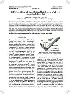
Disturbances wind speed, Solar Outside Outside … … CO2 concentration, radiation temperature humidity etc

… …

Inside (Tin(t) ) temperature

heating (Qheater(t)) ventilation (VR(t))

Crops

spraying (Qfog(t))

CO2 concentration

CO2 injection

Inputs

Inside (Hin(t)) humidity

Greenhouse

Outputs

Figure 1. Greenhouse climate dynamic model In order to effectively validate the performance of the proposed algorithm below, the considered greenhouse analytic expression is based on the heating/cooling/ ventilating model in this work, which can be obtained from many extant literatures [5, 24]. It can be summarized in the functional block diagram given in Figure 1. Considering the related high costs, CO2 supply systems have not an extensive use, therefore the related variables are not taken into account in this work. To simplify the model, we consider only some primary disturbance variables, such as solar radiation, outside temperature and humidity. According to the above analysis, the state

358

RBF Network Based Nonlinear Model Reference Adaptive PD Controller Design for Greenhouse Climate* Hai-Gen Hu, Li-Hong Xu, Rui-Hua Wei, Bing-Kun Zhu

equations have been formed based on the laws of conservation of enthalpy and matter, and the dynamic behavior of the states is described by using the following differential equations [24]:   dTin (t ) 1 Q (t )  Si (t )  Q fog (t )   VR (t )  UA Tin (t )  Tout (t )  dt C pVT heater C pVT   VT

(1)

dH in (t ) 1 1 E (Si (t ), H in (t ))  VR (t ) H in (t )  H out (t )  Q (t )  dt VH fog VH VH

(2)

Tin Tout is the indoor/outdoor air temperature ( ℃ ), H in H out is the interior/exterior humidity ratio (g[h2O]/kg [dry air]), UA is the heat transfer coefficient of enclosure (W/K), V is the geometric volume of the greenhouse (m3),  is the air density (1.2kg[air]m-3), C p is the where

specific heat of air (1006Jkg-1K-1),

Qheater is the heat provided by the greenhouse heater (W),

Q fog is the water capacity of the fog system (g[H2O]s-1), S i is the intercepted solar radiant

 is the latent heat of vaporization (2257Jg-1), VR is the ventilation E Si (t ), H in (t ) is the evapotranspiration rate of the plants (g[H2O]s-1). VT

energy (W/m2[ground]) , rate (m3[air]s-1),

VH are the active mixing air volumes of the temperature and humidity, respectively. Generally speaking, VT and VH are as small as 60%-70% of the geometric volume V of the greenhouse owing and

to short circuiting and stagnant zones exist in ventilated spaces. It is also worth noticing that, to a first approximation, the evapotranspiration rate

E Si (t ), H in (t )

is in most part related to the intercepted solar radiant energy, through the following simplified relation:

E S i (t ), H in (t )    T

S i (t )



  T H in (t )

(3)

where  T is an overall coefficient to account for shading and leaf area index, dimensionless and  T is the overall coefficient to account for thermodynamic constants and other factors affecting evapotranspiration (i.e., stomata, air motion, etc.) [24].

2.2. Greenhouse climate control problems The climate model provided above can be used in all seasons, and two variables have to be controlled namely the indoor air temperature and the humidity ratio through the processes of heating ( Qheater (t ) ), ventilation ( VR (t ) ) and fogging ( Q fog (t ) ). For summer operation in this work,

Qheater (t ) is set to zero. The purposes of ventilation are to exhaust moist air and to

replace it with outside fresh air, to control high temperatures caused by the influx of solar radiation, to dehumidify the greenhouse air when the humidity of the outside air is very low, to provide uniform air flow throughout the entire greenhouse, and to maintain acceptable levels of gas concentration in the greenhouse. Fogging systems (such as misters, fog units, or roof sprinklers) are primarily used for humidification of the greenhouse. In fact, fogging system also plays a cooling role due to evaporative cooling. Moreover, fresh air must be continually ventilated into the greenhouse, while warmed and humidified air to be exhausted. When humidifying is occurred under sunny conditions, ventilation is necessary since the greenhouse would soon become a steam bath without providing fresh dry air.

3. Design of Model Reference Adaptive PD Controllers for Greenhouse Climate 3.1. RBF network structure RBF, presented by J. Moody and C. Darken [25], emerged as a variant of artificial neural network in late 80's. RBF neural networks have an input layer, a hidden layer and an output layer. The neurons in the hidden layer contain Gaussian transfer functions whose outputs are inversely proportional to the distance from the center of the neuron. The architecture of a typical RBF network is shown in Figure 2.

359

RBF Network Based Nonlinear Model Reference Adaptive PD Controller Design for Greenhouse Climate* Hai-Gen Hu, Li-Hong Xu, Rui-Hua Wei, Bing-Kun Zhu h1

I1

w11



ym1



y mL

wL1

h2

I2

w12

wL2 w1M hM

IN Input Layer

Hidden Layer

wLM Output Layer

Figure 2. Architecture of a RBF network Each input node is corresponds to an element of the input vector

I in  R n , and each hidden

node implements a radial activated function, which consists of local perception nodes. The Gaussian activation function for RBF network is given by:

 I Cj h j  exp   2 j 

Where

   

j  1,2,, M

(4)

I  I1 , I 2 ,, I N  is the input feature vector, M is the number of hidden nodes,

C j  [c j1 , c j 2 ,, c jN ] is N-dimensional center parameter of the jth hidden node, symbol  denotes the Euclidean norm, and

j

is the positive center width parameter.

The output nodes implement a weighted sum of hidden node outputs as follows: M

y mi   ij h j

i  1,2,, L

(5)

j 1

where

ij

is the connection weight of the jth hidden node to the the ith output node, and L is

the number of output nodes.

3.2. Control strategy Notice that the greenhouse dynamic system mentioned above, it is a two-input and two-output continuous time nonlinear system. In order to simulate its behavior on a digital computer, we adopt a fourth-order Runge-Kutta method with a small enough integration step. Hence, considering a typical digital positional PD control algorithm is generally given as:

u (k )  K p ec (k )  K d

ec (k )  ec (k  1) ts

where k and ts is iterative step and sampling time, respectively.

(6)

K p and K d are the gains of

the proportional and derivative terms of a PD controller, respectively. Combining RBF network with the conventional PD controller, we employ a hybrid model reference adaptive control strategy, and its structure is shown in Figure 3. To avoid the windup caused by the interaction of integral action and saturations, we adopt limiters on the control law variations so that the controller output never exceeds the actuator limits, given as follows:

 0  ui (k )   uilim u (k )  i where

if ui (k )  0, if ui (k )  uilim , otherwise.

(i  1,2)

uilim (i=1,2) represent the maximum ventilation rate and the maximum water capacity of

the fog system, respectively. The corresponding reference model is represented as follows:

yr (k )  0.35 yr (k  1)  0.65r (k )

(7)

360

RBF Network Based Nonlinear Model Reference Adaptive PD Controller Design for Greenhouse Climate* Hai-Gen Hu, Li-Hong Xu, Rui-Hua Wei, Bing-Kun Zhu

r1(k)

yr1 (k )

Reference Model

PID Controller I

y1 ( k )

u1(k)

ym1(k)

Jacobian

em1(k)

Greenhouse Climate Model

RBF NNI

Jacobian

PID Controller II

ec1(k)

saturation

ym2(k)

saturation

em2(k)

y 2 (k )

u2(k)

ec2 (k)

Reference

yr2 (k)

Model r2(k) Figure 3. Block diagram of the greenhouse climate control system

3.3. Adjusting algorithm of adaptive PD RBF network is used to tune the parameters of the conventional PD controller through Jacobian information. The corresponding formulas are given as follows. The error signal is defined as (8) ec (k )  yr (k )  y(k ) The inputs of adaptive PD

xc (1)  ec (k ) xc (2)  ec (k )  ec (k  1) The control signal is updated by Eq. 6. The energy function

(9) (10)

E (k ) is defined as

1 E (k )  ec (k ) 2 2

(11)

and the parameters of PD are updated as:

K p (k )  K p (k  1)  K p (k )   ( K p (k  1)  K p (k  2))   K p (k  2)  K p (k  3)

(12)

K d (k )  K d (k  1)  Kd (k )   ( K d (k  1)  K d (k  2))   Kd (k  2)  K d (k  3)

(13) where



and



are the momentum factors. The corresponding

K p (k ) and K d (k ) are adjusted

based on the negative gradient method as follows:

K p  c

E E y u y  c  c ec (k ) xc (1) K p y u K p u

(14)

E E y u y  c  c ec (k ) xc (2) (15) K d y u K d u Where  c is the learning rate parameter; y u is the Jacobian information of the controlled plant, K d  c

which can be achieved by RBF network identification as follows:

c ji  u (k ) y(k ) ym (k ) M    j h j u (k ) u (k )  2j j 1

(16)

3.4. Identification algorithm of RBF neural network The structure of RBF network identification is shown in Figure 4, where input and output of identifier, respectively,

u (k ) and y(k ) represent

y m (k ) is output of RBF network.

361

RBF Network Based Nonlinear Model Reference Adaptive PD Controller Design for Greenhouse Climate* Hai-Gen Hu, Li-Hong Xu, Rui-Hua Wei, Bing-Kun Zhu

The identification algorithm of Jacobian information of controlled plant is stated below. The performance index function of controller is defined as: u (k )

Greenhouse Climate Model

y (k )

em (k )

RBF NNI

ym (k)

Figure 4. Plant identification based on RBF network

1 E m ( k )  em ( k ) 2 2 where

(17)

em (k ) is the error signal between the plant actual output and RBF network output, which is

represented by

em (k )  y(k )  ym (k ) In order to minimize the error

(18)

em (k ) , a gradient descent method is adopted to modify weights, center

vectors and center width parameters. The update equations for the RBF network parameters are given as follows.

 j (k )  

Em (k ) E ( K ) ym (k )   m  em (k )h j  j (k ) ym (k )  j (k )

 j (k )   j (k  1)   j (k )   ( j (k  1)   j (k  2))    j (k  2)   j (k  3)  j (k )  em (k ) j h j

X Cj

 3j

xi  c ji

 2j

(20)

2

 j (k )   j (k  1)   j (k )   ( j (k  1)   j (k  2))    j (k  2)   j (k  3) c ji (k )  em (k ) j

(19)

(21) (22) (23)

c ji (k )  c ji (k  1)  c ji (k )   (c ji (k  1)  c ji (k  2))   c ji (k  2)  c ji (k  3) (24)

where  is an appropriate learning rate parameter, too low a learning rate makes the network learn very slowly, while too high makes the weights and objective function diverge, here, let  =0.4. Besides,

 and  can speed up convergence and help the network out of local minima. Here, the values of  and  are 0.05 and 0.01, respectively.

it is to be noted that

4. Experiments and Results In order to verify the efficiency and good performance of the proposed model reference adaptive PD control scheme, a series of simulations experiments are presented in the present section. For this example, we consider a greenhouse of surface area 1000 m2 and a height of 4 m. The greenhouse has a shading screen that reduces the incident solar radiation energy by 60%. The maximum water capacity of the fog system is 26 g[H2O]min-1m-3. Maximum ventilation rate corresponds to 20 air changes per hour (22.2 m3s-1). Parameter  T takes the value 0.129524267 and  T =0.015 kgmin-1m-2. The heat transfer coefficient is UA=25 kWK-1. The active mixing air volumes of the temperature and humidity are given as VT  VH  0.65V . Moreover, the initial values of indoor air temperature and humidity

362

RBF Network Based Nonlinear Model Reference Adaptive PD Controller Design for Greenhouse Climate* Hai-Gen Hu, Li-Hong Xu, Rui-Hua Wei, Bing-Kun Zhu

ratio are 32℃ and 18 g[H2O]/kg[air], respectively. Considering the external climatic fluctuation with a small range during short time, outdoor temperature

Tout , relative humidity H out and solar radiation

Tout(  C)

External disturbances 40 35

S i(W/m 2 )

w out(g/m3 )

30

0

40

80

120

160

200

240

280

320

0

40

80

120

160

200

240

280

320

0

40

80

120

160 200 Time (min)

240

280

320

20 15

350 300 250 200 150

Figure 5. Changes of outdoor climate

S i change in random ways as shown in Figure 5 to represent external disturbances. In this experiment, the ability of adaptive, tracking and smooth closed-loop response to set-point changes is demonstrated. To draw a comparison with the proposed method, we adopt another traditional adaptive PD control method based on RBF neural network, which has not any difference from the proposed method but not to using a reference model. We consider a pair of square-wave reference inputs to test its control performance. Indoor air temperature set-point changes between 32 and 21 ℃ every 2000 seconds, where the humidity ratio set-point changes between 18 and 23g[H2O]/kg[air] (which corresponds to a relative humidity change between 60% and 76%). The corresponding responses for set-point square-wave changes in temperature and humidity ratio are shown in Figure 6. The results show that the model reference adaptive PD method is superior to the adaptive PD control method based on RBF neural network, and it has better adaptive and tracking performance. Table 1 shows the mean errors and standard deviations of temperature ( Tin ) and humidity ( H in ). As can be seen, the values of mean error and standard deviation by adopting MRAC method is smaller than the adaptive PD control method. In addition, Figure 7 shows that the corresponding control signals of the two methods vary with the set-point changes during the tuning process. The results show that the MRAC method provides smoother control signals than the traditional adaptive PD control method, and it can avoid the serious oscillating of the actuators. From the above analysis, the proposed control scheme is superior to the traditional adaptive PD control scheme based on RBF neural network, and it has good adaptability, strong robustness and satisfactory control performance. Table 1. Comparison of control error for the two methods during the tuning and control process, in which Mean and Std. represent the mean errors and standard deviation, respectively Adaptive PD control MRAC Mean Std.

Tin (℃)

H in ( g/kg)

Tin (℃)

H in ( g/kg)

-1.1934 2.9374

0.8267 1.3876

-0.6335 1.8954

0.4241 0.8798

5. Conclusion

363

RBF Network Based Nonlinear Model Reference Adaptive PD Controller Design for Greenhouse Climate* Hai-Gen Hu, Li-Hong Xu, Rui-Hua Wei, Bing-Kun Zhu

In this paper, a model reference adaptive PD control scheme based on RBF neural network is presented for the greenhouse climate control problem. A model, characterized with nonlinear conservation laws of enthalpy and matter between numeroReference inputs and Greenhouse outputs

(a)

30

Tin(  C)

Tin( C)

30

25

20

0

40

80

120

160 200 time(min)

240

280

25

20

320

24

24

22

22

w in(g/m3 )

w in(g/m3 )

Reference inputs and Greenhouse outputs

(b)

20 18

0

40

80

120

160 200 time(min)

240

280

320

0

40

80

120

160 200 time(min)

240

280

320

20 18

0

40

80

120

160 200 time(min)

240

280

320

(a) adaptive PD control method based on RBF NN (b) Model reference adaptive PD control method Figure 6. Tracking trajectory of square-wave for temperature and humidity ratio V R (m 3 [air]/s)

V R (m 3 [air]/s)

(b)

Control signals

(a) 25 20 15 10 5 0

0

40

80

120

160

200

240

280

15 10 5 0

40

80

120

0

40

80

120

160

200

240

280

320

160 200 time(min)

240

280

320

30

Q fog (g[H2O]/s)

Q fog (g[H2O]/s)

20

0

320

30

20

10

0

Control signals 25

0

40

80

120

160 200 time(min)

240

280

320

20

10

0

(a) adaptive PD control method based on RBF NN (b) Model reference adaptive PD control method Figure 7. Variation of control signals during the tuning process

us system variables affecting the greenhouse climate, has been used to validate the proposed control scheme by tracking square-wave trajectory and being compared with the conventional adaptive PD control scheme based on RBF neural network. The results show that the proposed adaptive controller has a more satisfactory control performance than the conventional scheme, such as adaptability, robustness and set-point tracking. It can be applied in the nonlinear time-varying dynamical control systems like greenhouse climate system. Therefore, it may provide a valuable reference to formulate environmental control strategies for actual application in greenhouse production. The approach is not limited to greenhouse applications, but could easily be extended to other applications.

6. Acknowledgment This work was supported by the National Natural Science Foundation of China under the Grant No. 61174090, Common Weal Projects of Zhejiang Province, China under the Grant No. 2011C21002, and also by a grant from the Education Department of Zhejiang Province, China, and by BEACON (An NSF Science and Technology Center for the Study of Evolution in Action, Coop. Agmt.) of USA under the Grant NO. DBI-0939454.

7. References

364

RBF Network Based Nonlinear Model Reference Adaptive PD Controller Design for Greenhouse Climate* Hai-Gen Hu, Li-Hong Xu, Rui-Hua Wei, Bing-Kun Zhu

[1] Coelho, J. P., P. B. Moura Oliveira, and J. Boaventura Cunha, “Greenhouse air temperature predictive control using the particle swarm optimisation algorithm”, Computers and Electronics in Agriculture, vol. 49, no. 3, pp. 330-344, 2005. [2] Cunha, J. B., C. Couto, and A. E. B. Ruano, “A greenhouse climate multivariable predictive controller”, Acta Horticulturae N. 534, ISHS, pp. 269-276, 2000. [3] Piñón, S., E. F. Camachoa, B. Kuchen, and M. Peña, Constrained predictive control of a greenhouse. Computers and Electronics in Agriculture, vol. 49, no. 3, pp. 317-329,2005. [4] Arvanitis, K. G., P. N. Paraskevopoulos, and A. A. “Vernardos, Multirate adaptive temperature control of greenhouses”, Computers and Electronics in Agriculture, vol. 26, no. 3, pp. 303-320, 2000. [5] Pasgianos, G. D., K. G. Arvanitis, P. Polycarpou, and N.Sigrimis, “A nonlinear feedback technique for greenhouse environmental control”, Computers and Electronics in Agriculture, vol. 40, no. 1-3, pp. 153-177, 2003. [6] Lafont, F., and J. -F. Balmat, “Optimized fuzzy control of a greenhouse”, Fuzzy Sets Syst., vol. 128, no. 1, pp. 47-59, 2002. [7] Lafont, F., and J. F. Balmat, “Fuzzy logic to the identification and the command of the multidimensional systems”, International Journal of Computational Cognition, vol. 2, no. 3, pp. 21-47, 2004. [8] Miranda, R. C., E. Ventura-Ramos, R. R. Peniche-Vera, and G. Herrera-Riuz, “Fuzzy greenhouse climate control system based on a field programmable gate array”, Biosystems Eng., vol. 94, no.2, pp. 165-177, 2006. [9] Bennis, N., J. Duplaix, G. Enéa, M. Haloua, and H. Youlal, “Greenhouse climate modelling and robust control”, Computers and Electronics in Agriculture, vol. 61, no. 2, pp. 96-107, 2008. [10] Pucheta, J. A., C. Schugurensky, R. Fullana, H. Patiño, and B. Kuchen, “Optimal greenhouse control of tomato-seedling crops”, Computers and Electronics in Agriculture, vol. 50, no. 1, pp. 70-82, 2006. [11] Hu, H., L. Xu, B. Zhu, and R. Wei, “A Compatible Control Algorithm for Greenhouse Environment Control Based on MOCC Strategy”, Sensors, vol. 11, no. 3, pp. 3281-3302, 2011. [12] Omid M., “A Computer-Based Monitoring System to Maintain Optimum Air Temperature and Relative Humidity in Greenhouses”, Int. J. Agri. Biol., vol. 6, no. 5, pp.869-873, 2004. [13] Li, Y., N. Sundararajan, and P. Saratchandran, “Neuro-controller design for nonlinear fighter aircraft maneuver using fully tuned RBF networks”, Automatica, vol. 37, pp. 1293-1301, 2001. [14] Shifei Ding, Gang Ma, Xinzheng Xu, "A Rough RBF Neural Networks Optimized by the Genetic Algorithm", AISS, Vol. 3, No. 7, pp. 332-339, 2011. [15] Cai Guoqiang, Tong Zhongzhi, Xing Zongyi, "Modelling of Electrohydraulic System Using RBF Neural Networks and Genetic Algorithm", JCIT, Vol. 5, No. 7, pp. 29-35, 2010. [16] Nielsen, B., and Madsen, H., “Identification of a linear continuous time stochastic model of the heat dynamic of a greenhouse”, J. Agr. Eng. Res., vol. 71, no. 3, pp. 249-256, 1998. [17] Tap, R. F., “Economics-based optimal control of greenhouse tomato crop production”, PhD diss. Wageningen, Netherlands: Wageningen University, 2000. [18] Ghosal, M. K., G. N. Tiwari, and N. S. L. Srivastava, “Modeling and experimental validation of a greenhouse with evaporative cooling by moving water film over external shade cloth”, Energy and Buildings, vol. 35, no.8, pp. 843-850, 2003. [19] Javier Leal Iga, “Modeling of the Climate for a Greenhouse in the North-East of México”, Proceedings of the 17th World Congress.The International Federation of Automatic Control, The Netherlands. Seoul, Korea, pp. 9558-9563, 2008. [20] Fathi Fourati, and Mohamed Chtourou, “A greenhouse control with feed-forward and recurrent neural networks”, Simulation Modelling Practice and Theory, vol. 15, no. 8, pp. 1016-1028, 2007. [21] Trejo-Perea, M., G. Herrera-Ruiz, J. Rios-Moreno, R. C. Miranda, and E. Rivas-Araiza, “Greenhouse energy consumption prediction using neural networks models”, Int. J. Agric. Biol. vol. 11, no. 1, pp. 1-6, 2009. [22] He, F., and C. Ma, “Modeling greenhouse air humidity by means of artificial neural network and principal component analysis”, Comput. Electron. Agric., vol. 71S, no. S19-S23, 2010. [23] Cunha, J. B., “Greenhouse climate models: An overview”, In: EFITA 2003 Conference, 823-829. Debrecen, Hungary. 2003.

365

RBF Network Based Nonlinear Model Reference Adaptive PD Controller Design for Greenhouse Climate* Hai-Gen Hu, Li-Hong Xu, Rui-Hua Wei, Bing-Kun Zhu

[24] Albright, L. D., R. S. Gates, K. G. Arvanitis, and A. E. Drysdale. “Environmental control for plants on earth and in space”, IEEE control system magazine, vol. 21, no.5, pp. 28-47, 2001. [25] Moody, J., and C. J. Darken, “Fast learning in networks of locally tuned processing units”, Neural Computation, 1: 281-289, 1989.

366