Incremental RBF Network Models for Nonlinear ... - IEEE Xplore

Incremental RBF Network Models for Nonlinear Approximation and Classification Gancho Vachkov

Valentin Stoyanov

Nikolinka Christova

School of Engineering and Physics The University of the South Pacific (USP) Suva, Fiji Islands [email protected]

Department of Automatics and Mechatronics University of Ruse “Angel Kanchev” Ruse, Bulgaria [email protected]

Department of Automation of Industry, University of Chemical Technology and Metallurgy (UCTM) Sofia, Bulgaria [email protected]

Abstract—In this paper a multistep learning algorithm for creating a novel incremental Radial Basis Function Network (RBFN) Model is presented and analyzed. The proposed incremental RBFN model has a composite structure that consists of one initial linear sub-model and a number of incremental submodels, each of them being able to gradually decrease the overall approximation error of the model, until a desired accuracy is achieved. The identification of the entire incremental RBFN model is divided into a series of identifications steps applied to smaller size sub-models. At each identification step the Particle Swarm Optimization algorithm (PSO) with constraints is used to optimize the small number of parameters of the respective submodel. A synthetic nonlinear test example is used in the paper to analyze the performance of the proposed multistep learning algorithm for the incremental RBFN model. A real wine quality data set is also used to illustrate the usage of the proposed incremental model for solving nonlinear classification problems. A brief comparison with the classical single RBFN model with large number of parameters is conducted in the paper and shows the merits of the incremental RBFN model in terms of efficiency and accuracy. Keywords—multistep incremental model; radial basis function network; particle swarm oprimization; nonlinear approximation; classification

I. INTRODUCTION Radial Basis Function (RBF) Networks have been widely used in the last decade as a power tool in modeling and simulation, because they are proven to be universal approximators of nonlinear input-output relationships with any complexity [1,2,3]. In fact, the RBF Network (RBFN) is a composite multi-input, single output model, consisting of a predetermined number of N RBFs, each of them performing the role of a local model [3,4]. Then the aggregation of all the local models as a weighted sum of their output produces the nonlinear output of the RBFN. There are some important features that make the RBF networks diferent from the clasical feed forward networks, such as the well known multilayer perceptron (MLP), often called back-propagation neural network [1,2,5]. The most important difference is that the RBFN models are not

homogeneous in parameters. They have three different groups of parameters that need to be appropriately tuned, normally by using different learning (optimization) algorithms. This makes the total learning process of the RBFN more complex, because it is usually done in a sequence of several learning phases. This obviously may affect the accuracy of the produced model. In this paper we first analyse the internal structure and the properties of the classical RBFN model with a pre-determined number of RBF units and its respective learning algorithm, based on the Particle Swarm Oprimization (PSO) algorithm with constraints [6,7]. Then we propose a new learning algorithm for creating an incremental structure of the RBFN model that consists of a number of sub-models. The initial sub-model is a simple linear model, where all the subsequent sub-models are in the form of small size nonlinear RBFN models - RBFN models with a small fixed number of RBFs. The sub-models are identified separately in a sequence of identification steps, by using the PSO algorithm with inertia weight and constrains. Then the modeled output of the overal composite incremental model is easy to calculate as additive function of the outputs of all sub-models. The early ideas for creating of incremental type of models for the purpose of approximation have been explained in [8,9]. Other ideas for creating incremental type of models are given in [10,11,12] with most applications for classification.The idea of creating growing RBFN models is given in our work [13]. The difference between all those ideas and our proposed model here is that most authors are dealing with the problem of creating a single model that gradually improves its performance, when new eamples are available, by appropriate change in its structure or parameteers. Others authors are interested in gradual (incremental) improvement of the model based on the same training data set, by gradual increase of the model complexity (inserting new units or changing the internal structure and parameters). The proposed here idea of the incremental RBFN model is that this is not a single model, but rather a structure of submodels that gradually grows at each identification step, by insertion of a new sub-model. Thus a gradual improvement of the approximation ability of the overall composite model is achieved.

The performance of the proposed multi-step learning algorithm for creating incremental RBFN model is discused and analysed in the paper on two examples of nonlinear approximation and classification. An experimental comparison of the proposed model with the classical single RBFN model with large nimber of RBFs and respective paramees is also done in the paper. II. THE CLASSICAL RBF NETWORK MODEL Our objective is to create a model of a real process (system) with K inputs and one output based on a preliminary available collection of M experiments (input-output pairs) in the form:

{( X1 , y1 ),..., ( X i , yi ),..., ( X M , yM )}

(1)

Here X = [ x1 , x2 ,..., xK ] is the vector consisting of all K inputs for the system (process) under investigation. The measured output from the process is denoted by y . Then the predicted output, modeled by the RBF network is given, as follows: (2)

ym = f ( X, P )

associated with the outputs of the RBFs, including one additional offset weight w0 as seen in the figure. The output u of each RBF is calculated by the following Gaussian function in the K-dimensional input space:

⎛ K ⎞ u = exp ⎜ − ∑ ( x j − c j ) 2 (2σ 2 ) ⎟ ∈ [0,1] ⎝ j =1 ⎠

(4)

Is easy to realize that each RBF is determined by K+1 parameters, namely the K-dimensional vector of the Centers (locations) C = [c1 , c2 ,..., cK ] of the RBFs in the Kdimensional space and the scalar Width (spread) σ . An example of a RBF with assumed scalar width of σ = 0.15 and a center C = [0.4,0.6] in the two-dimensional space (K=2) is shown in Fig. 2. It is straightforward to calculate the number L of all parameters that characterize the classical RBF Network from Fig. 1 with K inputs and N RBFs, as follows:

L = N × K + N + ( N + 1) = N × K + 2 × N + 1

(5)

Vector P = [ p1 , p2 ,..., pL ] represents the list of all L parameters participating in the RBFN model. They will be explained and analyzed later in the text. The classical RBFN model is described as a three layer structure, namely input, hidden and output layer as shown in Fig. 1.

Fig. 2. Example of a RBF with K=2 Inputs, center at [0.4, 0.6] and a single width σ = 0.15.

Fig. 1. Structure of the classical Radial Basis Function Network with K inputs and N RBFs.

The modeled output of the RBF network with preliminary given number of N Radial Basis Functions is calculated as a weighted sum of the outputs from all N RBFs:

ym = w0 +

N

∑wu

i i

(3)

i =1

Here ui , i = 1, 2,..., N are the outputs of the RBFs with K inputs

x1 , x2 ,..., xK and wi , i = 0,1, 2,..., N are the weights

All these parameters constitute the vector of Parameters P from (2). It is worth to note here that these parameters are heterogeneous in nature, unlike the parameters of the classical back-propagation neural network (the multilayer perceptron) where all parameters are homogeneous and represent one category – the connection weights between the units (neurons). In the classical RBF Network all L parameters form 3 different sets (categories): the set C of Centers with NxK parameters; the set σ of all N Widths (spreads) and the set W of N+1 Weights, as follows:

P = [ p1 , p2 ,..., pL ] = C ∪ σ ∪ W

(6)

It is seen from (5) that the number L of all parameters in the RBFN model will grow rapidly with increasing the size of the model, namely the number N of RBFs and the number K of the inputs. This creates the challenging task of performing a computationally expensive tuning procedure for all parameters of the RBFN model with large size. Such multidimensional optimization problem becomes even more complex when the goal is to guarantee that we have achieved the global minimum for the approximation error.

application. The accent in this paper is focused mainly on the idea and performance of the incremental RBFN model.

III. TUNING THE PARAMETERS OF THE RBFN MODEL BY PARTICLE SWARM OPTIMIZATION WITH CONSTRAINTS The problem of tuning the parameters of the RBF network has been investigated by many authors for a long time by using different learning algorithms that include separate or simultaneous tuning of the 3 groups of parameters [3,4,5] and by applying different optimization approaches. In this paper we use a nonlinear optimization strategy for simultaneous learning of all three groups of parameters in (6) and for this purpose we use a modified version of the Particle Swarm Optimization (PSO) algorithm with constraints, as described in the sequel. The PSO algorithm [6] belongs to the group of the multiagent optimization algorithms. It uses a heuristics that mimics the behavior of flocks of flying birds (particles) in their collective search for a food. The general concept here is that a single bird has not enough power to find the best solution, but in cooperation and exchanging information with other birds in the neighborhood it is likely to find the best (global) solution. The swarm consists of a predetermined number n of particles (birds) that exchange information during their cooperative behavior. More details and a very good overview of the PSO algorithm with its most popular modifications are given in [7]. The classical version of the PSO algorithm in [6] does not impose any constraints (boundaries) on the search of the “birds” in the K-dimensional input space, so it is an unconstrained optimization. The reason for such assumption is that birds should be free and active to explore the whole unlimited space until eventually they find the global optimum. However, many practical engineering problems require certain constraints (limits) to the parameters [ x1 , x2 ,..., xK ] in the input space, in order to produce a physically meaningful optimal solution. This represents a constrained optimization procedure, which produces the so called conditional optimum that can be practically implemented. In order to achieve such plausible practical solutions, we have made here a slight modification in the original version of the PSO algorithm with inertia weight that applies constraints as minimum and maximum on all input parameters, as follows:

xi min ≤ xi ≤ xi max , i = 1,2,...,K

(7)

Then the idea of the constrained optimization is very simple. The input parameter that has violated the input space is moved back to its boundary value from (7), as follows:

if ( xi < xi min ) then xi = xi min ; i = 1, 2,...K if ( xi > xi max ) then xi = xi max ; i = 1, 2,...K

IV. CRITERIA FOR OPTIMIZATION OF THE RBFN MODEL Depending on the purpose of using the RBFN model, there could be different optimization criteria, as described below. A. Criterion for Optimization of the RBFN Model when used for Nonlienear Approximation When the RBFN model is used for performing a nonlinear approximation (also known as a regression problem), the most popular optimization criterion is to minimize the approximation error RMSE between all M real measured outputs and the respective modeled (predicted) outputs by the RBFN model, as follows:

RMSE =

M

∑( y − y ) i

im

2

→ min

(9)

i =1

Here the problem is how to properly tune all parameters from (6) so that to achieve the global minimum. B. Criterion for Optimization of the RBFN Model when used as Universal Nonlinear Approximator When a classification problem has to be solved, a slight modification of the statement of the problem is needed. Here the outputs of all M samples (experiments) in the training set are not real values, but rather integer numbers that represent T ordered classes, labeled as consequent numbers: t = 1,2,..., T . Since the classical RBFN model produces real valued outputs, as in (3), we need a kind of a post processing procedure in order to transform the RBFN model into a respective Classifier that makes a decision for a certain class at each sample. We use the following simple quantization procedure for this purpose: 1) Check the truth value of the predicted output from the Classifier (the RBFN model) for every sample i = 1,2,…,M from the training set with the respective known true class t, t=1,2,…,T, as follows: - Calculate the difference between the true class t and the predicted real value yi for the i-th sample: Δ i = t − yi -

For t = 2,3,…,T-1 check the following:

if ( Δi > - 0.5 ∧ Δ i ≤ 0.5) then : class t is true -

(8)

In such way, at the next iteration in the search of the PSO , a new velocity (step) with different direction will be generated. As a result the particle is likely to escape from being trapped in the “prohibited” area beyond the boundary. This often takes not only one, but a few trials (iterations). We should note here that the PSO algorithm with its modifications is by no means the only optimization tool that could be used for tuning the parameters of the RBFN model. Some other meta-heuristic methods, such as those described in [14] and [15] have also their own merits and strengths in

1 M

For t = 1 check the following:

if (Δ i ≤ 0.5) then : class t is true -

For t = T check the following:

if (Δ i > - 0.5 ) then : class t is true 2) Count the number q of all misclassified samples from all M available samples (experiments). Then, the proposed criterion for classification is in the form of classification error Cerr. This is a real value bounded between 0.0 and 1.0 that shows the fraction of all misclassified samples from the whole list of M training samples, namely:

Cerr = q / M ; 0 ≤ q ≤ M ; 0.0 ≤ Cerr ≤ 1.0

(10)

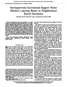
Further on in the text an illustration of this criterion for optimizing the parameters of the RBFN is given based on a real classification example. V. THE MULTISTEP ALGORITHM FOR LEARNING THE INCREMENTAL RBFN MODEL The proposed in this paper incremental RBFN model is a kind of a composite model, consisting of several sub-models that are identified one after another, in a sequence of several identification steps. These sub-models include one initial submodel and a number of subsequent incremental sub-models. Thus the whole incremental RBFN model is created in a multistep identification process. The only available information before the start of the identification is the training data set (1) consisting of M input-output samples. The block diagram that visualizes the multistep identification procedure for creating the incremental RBFN model is shown in Fig. 3. The whole multistep learning process in this figure is aimed at creating one initial sub-model, denoted as MOD0 and two incremental sub-models, denoted as MOD1 and MOD2.

the model will gradually increase. However, the good point here is that there is no much increase in the computational cost, because each identification step is performed on one sub-model only that has a small size (small number of parameters). Since the identification process is actually an optimization procedure, this means that at each step, a small size optimization procedure will be run, compared to the full size optimization with much larger large number of parameters, if we attempt to create a “one-time” full-size model. A. The Initial Identification Step At the initial identification step we create a relatively rough model that is aimed at capturing the most basic (general) inputoutput relationships. It is obvious that the best and yet simple model for such purpose would be the linear sub-model, denoted as MOD0 in Fig. 3. In case of a process with Kdimensional input vector X, this model has a total number of K+1 parameters and is represented by the following equation: K

yi m 0 = a0 + ∑ a j xi j , i = 1,2,..., M .

(11)

j =1

According to the notations in Fig. 3 the model error after the initial identification step will be:

ei 0 = yi m 0 − yi , i = 1,2,..., M

(12)

A graphical illustration of the result of the initial identification step is depicted in Fig. 4. The approximation error (9) at this step is denoted as RMSE0 and is used as a measure of the model quality at this initial step. The errors (12) for all M experiments create the so called error vector E0, which is saved for further use in the next incremental identification step.

Fig. 3. The multistep identification procedure for creating the Incremental RBFN model.

It is worth noting that the initial sub-model MOD0 is a compulsory first element in the structure of the composite incremental RBFN model, while the number of the subsequent incremental sub-models MOD1, MOD2, … is variable and decided by the user or controlled by the desired identification accuracy. The general idea of creating the composite incremental model is that each new sub-model that is being added to the structure of the current incremental model will contribute to decreasing the approximation error RMSE (9) of the whole model with the current collection of already identified submodels. The process of adding additional incremental submodel continues until the desired value for the RMSE is obtained, or until the predefined number of incremental submodels by the user is reached. It is obvious that in this multistep procedure of subsequent identifications, the complexity of the whole composite incremental RBFN model and the number of all parameters in

Fig. 4. Ilustration of the variables from the initial identification step.

B. The Subsequent Incremental Identification Steps In the first incremental identification step an additional submodel MOD1 is created, according to Fig. 3. This could be a relatively simple, but preferably a non-linear model that should be able to decrease the approximation error RMSE0, produced at the previous initial identification step. In this paper we propose to use for such purpose RBFN models with a relatively small (preliminary fixed) number of RBFs (e.g. N = 3,4, 5) as incremental sub-models, because they are both relatively simple and nonlinear in nature. In the first incremental identification step, the inputs are taken from the vector X of the original inputs, while the

outputs needed for the identification are taken from the error vector E0, produced in the previous initial identification step. As a result, the following new errors are obtained at the end of the first identification step: ei1 = yi m1 − ei 0 , i = 1,2,..., M (13) The new approximation error (9) from the whole incremental model will be denoted as RMSE1. The errors (13) for all M experiments from this step create the error vector E1 that is saved for further use in the subsequent identification step In a similar way, at the second incremental identification step a new incremental sub-model MOD2, according to Fig. 3 is created with the following new errors:

ei 2 = yi m 2 − ei1 , i = 1,2,..., M

(14)

Here the new approximation error (9) from the whole incremental model will be denoted as RMSE2. The errors (14) for all M experiments from this step create the error vector E2 that will be used in the subsequent identification step An illustration of the above explained two incremental identification steps is given in Fig. 5 and Fig. 6.

RMSE 0 ≥ RMSE1 ≥ RMSE 2 ≥ ... ≥ RMSEr

(15)

For all identification steps in the above multi-step procedure we use in this paper the PSO algorithm, with the details given in Sections III and IV.

C. Calculation of the Incremental RBFN Model From the above equations (11) - (14) it is straightforward to conclude that for each given input X, the final output of the incremental RBFN model will be an additive function of the outputs of all r+1 sub-models, included in its structure, i.e. r

ym i = ∑ yi mj , i = 1,2,..., M

(16)

j=0

The calculation structure of the incremental RBFN model is illustrated in Fig. 7. In the next Sections some illustrations and performance evaluation of the proposed Incremental RBFN model is given.

Fig. 7. The procedure for calculting the composite Incremental RBFN model.

VI. PERFORMANCE OF THE INCREMENTAL RBFN MODEL ON A TEST NONLINEAR EXAMPLE Fig. 5. Illustration of the variables from the first incremental step.

We have created a synthetic nonlinear model, consisting of 5 RBFs as a typical test example of a nonlinear process with K=2 inputs and one input. The test example is illustrated in the 3-dimensional plot in Fig. 8. Then the nonlinear model was used for generating different sets of Input-Output data that can be applied for solving several approximation and classification problems. Further on in the text we use a generated data set from this example for performance evaluation of the proposed incremental RBFN model in solving nonlinear approximation problem.

Fig. 6. Illustration of the variables from the second incremental step.

In a summary, if we would like to create an incremental RBFN model with r steps (r >0), the result will be a composite model that consists of r+1 sub-models: one linear sub-model MOD0 and r non-linear RBF sub-models MOD1, MOD2,…,MODr. Then the apprroximation error RMSE will be monotonously decreasing function with each incremental step, as follows:

Fig. 8. The response surface of the test nonlinear example used for nonlinear approximation and performance evaluation.

A training set of M = 400 randomly generated inputs and their respective calculated outputs is shown in Fig. 9. It is used for illustration of the approximation capabilities of the proposed incremental RBFN model. Fig. 10 shows the produced initial linear sub-model and Fig. 11 depicts the error surface after the initial identification step. The initial approximation error is: RMSE0 = 3.4491.

(r=2). It is seen that the error drops rapidly to RMSE2 = 0.3207 and convergence is fast and stable.

Fig. 12. The response surface of the sub-model MOD1 created at step 1 of the incremental identification. The approximation error is: RMSE1 = 0.5267. Fig. 9. The training set of 400 random generated inputs for the test nonlinear example, used in the simlations.

Fig. 10. The response surface of the initial linear model MOD0. The approximation error atvthis initial step is: RMSE0 = 3.4491.

Fig. 13. Convergence resuts for RMSE2 from the PSO algorithm used for training the incremental sub-model MOD2 for nonlinear approximation.

Finally, Fig. 14 show the simulation results from comparison of the performance of three incremental RBFN models with different structure. They use sub-models with different complexity, namely with 3, 4 and 5 RBFs. As expected, the more complex sub-models with 5 RBFs have produced a better (smaller) approximation error and leaded to a faster convergence of the RMSE, with just a few (r = 3,4) incremental steps.

Fig. 11. The response surface of the error vector RMSE0 after the initial identification step.

Fig. 12 is an illustration of the approximation performance of the composite incremental model consisting of the initial linear sub-model MOD0 and one only incremental sub-model, i.e. MOD1. The approximation error drops significantly to RMSE1 = 0.5267. The high level of resemblance between the original nonlinear surfaces in Fig. 8 (the original example) and the first-step approximation surface in Fig. 12 is obvious. Fig. 13 shows the performance of the PSO algorithm for creating the second incremental sub-model MOD2 in step 2

Fig. 14. Comparison results of three incremental RBFN models that use different incremental sub-models with 3, 4 and 5 RBFs respectively.

For comparison, the simpler sub-models with 3 and 4 RBFs needed more identification steps (up to r= 8 shown here) to achieve a similar level of approximation error. This means that a desired approximation error could be achieved in two ways, namely by using more complex sub-models and small number of identification steps, or by using simpler submodels with larger number of steps. Here an appropriate trade-off should be made, considering two additional factors: the CPU time and the total number of parameters of the model. Another comparison of the approximation results from the composite incremental RBFN models in Fig. 14 was made with the results from a single large RBFN model with similar number of parameters. Here a single (classical) RBFN model with 20 RBFs was used with a total number of parameters: 20x2 + 20 + 21 = 81, according to (5). The respective number of parameters of the 3-step (r=3) incremental RBFN model, consisting of one linear and 3 nonlinear sub-models with 5 RBFs is: 3 + [5x2+5+6]*3 = 3 + 21*3 = 63+3 = 66. In this case the simulation results showed a clear advantage of the proposed incremental RBFN model, as follows: the approximation error RMSE of the single classical RBFN model was within the range [0.5767, 1.0370] for 6 different runs of the PSO algorithm with slight change in the tuning parameters, while the achieved RMSE from the incremental RBFN model with r=3 sub-models was as low as 0.2665. The above simulations serve as an experimental proof for the better average accuracy and efficiency (in term of a CPU time) of the proposed incremental RBFN model, compared with the classical single RBFN model. We should note here that this is not a rigorous proof and may lead to slight variations in the results, because of the stochastic nature of the PSO algorithm (6) and the chosen tuning parameters. In all of the above simulations, a PSO algorithm with inertia weight from [7] was used, with our added idea for constrained optimization (7) and (8), explained in Section III. VII. PERFORMANCE EVALUATION OF THE INCREMENTAL RBFN MODEL FOR CLASSIFICATION In this section we analyze the performance of the proposed incremental RBFN model for solving classification problems. In [16] two real datasets have been used for testing three different data mining methods for classification, namely the Multiple Regression (MR), Back-propagation Neural Networks (NN) and Support Vector Machines (SVM). The two datasets are related to the red and white variants of the Portuguese "Vinho Verde" wine. They comprise of 1599 samples for the red wine and 4898 samples for the white wine. The datasets are publicly available in UCI Machine Learning Repository [17]. The authors in [16] conclude that the SVM achieves the best classification performance with the least classification error. In these data sets there are 11 input attributes that can be used as possible features for classification. They represent different real variables based on physicochemical laboratory tests. Some of the attributes are correlated, which encourages

researchers to apply some techniques for feature selection before the actual classification. The output variable (based on sensory data) is the quality of the wine, expressed as an integer value between 0 and 10. The worst quality is marked as 0 and the best wine quality is denoted by 10. The classes are ordered from 0 to 10, but are not balanced, i.e. there are much more normal wines than excellent or poor ones. The histogram that shows the distribution of all classes for the complete data set for the red wine with 1599 samples is depicted in Fig. 15. It is seen from the figure that some classes are not represented by any samples. Therefore they have been omitted in our simulations and only the real existing classes: 3,4,5,6,7 and 8 have been taken into consideration. Then all the “active classes” 3,4,5,6 and 7 were renumbered as “new classes” with respective new labels: 1,2,3,4,5 and 6. Their distribution can also be seen in Fig. 15.

Fig. 15. The histogram of all 6 new classes for the data set of red wine with 1599 samples.

Before training the proposed incremental RBFN model as a nonlinear classifier for this problem, we have conducted a simple feature selection procedure, as follows. From the whole list of 11 input attributes, the input 8 (wine density) was excluuded, since it has very small variation throughout the whole range of samples [0.9901, 1.0037]. The remaining 10 inputs have been normalized in the range of [0.0, 1.0] and then used for trainning of the nonlinear classifier (the incremental RBFN model) and for classification of the test data into given number of 6 classes. The first 1200 samples from the entire data set of 1599 samples were used as a training set for creating the nonlinear classifier. Here an Incremental RBFN model with r=1 and r=2 ncremental sub-models was used and the following results were obtained: the initial linear model (r=0) achiewed an overall classificationn error of Cerr0=0.6307 (757 misclassifications), according to the criterion (10). The incremented RBFN model with one additional sub-model (r=1) achieved an improved classification error of Cerr1 = 0.4017 (482 misclassifications). Adding more identification steps (r=2,3…) in the incremental RBFN model almost did not improve the clasification results, which suggests that we are around the boundary of the classification accuracy for this “difficult” real data example. The parameters of the PSO algorithm used for identifying the fist incremental RBFN model with r=1 were, as follows,

according to the notations in [7]: Number of particles: n = 20; Number of iterations: ITmax=2200; Initial inertia weight: ω1 = 0.95; Final inertia weight: ω2 = 0.25; Acceleration coefficients: ψ1 = 1.80; ψ2 = 1.70; Maximal size of the velocity (step): υmax = 0.20. When aplying the incremental RBFN model as a nonlienar classifier for the test data set (the remaining 399 samples ) the classification error has slightly increased to Cerr = 0. 4812 (192 misclassifications). Here a direct comparison of our classification results with those of the authors in [16] is difficult to be made, because we have excluded one of the input attributes (input 8) and also have not used a k-fold cross-validation strategy for classification. Our classification results are based on only one division of all data into a training data set with 1200 samples and a test data with the remaining 399 samples. Nevertheless the classification results are promissing for the incremental RBFN model, since the obtained classification error is close to the mean absolute deviation MAD=0.46, obtained in [16]. The main purpose in our simulations was to show the capability of the proposed incremental RBFN model to gradually improve its accuracy by adding more sub-models in its structure. VIII. DISCUSSIONS AND CONCLUSIONS A multistep learning algorithm for creating incremental RBFN model is proposed in this paper. It creates a kind of a composite model that consists of one initial linear sub-model and r incremental sub-models, each of them in the form of relatively simple RBFN models that are subsequently added to the previous model structure. The identification of the submodels is done by the PSO algorithm with inertia weight and constrains on the input parameters. Important feature of the final incremental RBFN model is that the modeled output is an additive function of the outputs of all individual r+1 sub-models namely: one linear and r nonlinear sub-models. As a result, the approximation error RMSE gradually decreases with increasing the number of the sub-models. Simulation results in the paper have shown that the proposed incremental RBFN model has a flexible structure that allows achieving approximation results with a predetermined (desired) accuracy, by gradually increasing the number of the sub-models. Two simulations have been conducted in this paper, as follows: approximation of a test nonlinear example, as well as classification of a real Wine Quality data set into 6 classes. These simulations have shown the merits of the proposed incremental RBFN model. The most important merit is that the incremental model performs implicitly a kind of decomposition of the original complex single RBFN model into a series of simpler RBFN models with smaller size, thus alleviating the overall identification task by improving the final approximation accuracy with a lower computation cost.

The future directions of this research are aimed at solving some currently existing problems with this model. First, the problem of automatic selection of the tuning parameters for the PSO algorithm should be solved in a satisfactory way, so that to decrease the variations in the optimization results between the different runs, as well as to increase the probability of finding global optimum solutions. Second, a more detailed and elaborated method is needed for possible automatic selection of the boundaries between the different classes, when the incremental RBFN model is used as a nonlinear classifier. This could significantly improve the classification accuracy when dealing with large and noisy data sets. REFERENCES [1] [2] [3]

[4]

[5]

[6]

[7] [8] [9] [10]

[11]

[12]

[13]

[14]

[15]

[16]

[17]

T. Poggio and F. Girosi. 1990. “Networks for approximation and learning”. Proceedings of the IEEE, 78, 1990, pp. 1481-1497. J. Park and I.W. Sandberg,. “Approximation and Radial-Basis-Function Networks”. Neural Computation, 5, 1993, pp. 305-316. M. Musavi, W. Ahmed, K. Chan, K. Faris, and D. Hummels, . 1992. “On the training of Radial Basis Function Classifiers”, Neural Networks, 5, 1992, pp. 595-603. R. Yousef, R. “Training Radial Basis Function Networks using reduced sets as center points”. International Journal of Information Technology, 2, 2005, pp. 21-27. J.-X. Peng, K. Li and G. W. Irwin, “A novel continuous forward algorithm for RBF neural modeling,” IEEE Transactions on Automatic Control, Vol. 52, No. 1, 2007, pp. 117-122. R.C. Eberhart J. Kennedy. “Particle Swarm Optimization”, in: Proc. of IEEE Int. Conf. on Neural Networks, Perth, Australia, 1995, pp. 1942– 1948. R. Poli, J. Kennedy and T. Blackwell, “Particle Swarm Intelligence. An Overview”, Swarm Intelligence, vol. 1, pp. 33-57, 2007. B. Fritzke, “Fast learning with incremental RBF Networks”, Neural Processing Letters, Vol.1, No. 5, 1994, pp. 1-5. J.C.Platt, “A resource-allocation network for function interpolation”, Neural Computation, Vol. 3, No. 2, 1991, pp. 213-225. K. Yamauchi, N. Yamaguchi, and N. Ishii: “Incremental learning methods with retrieving of interfered patterns,” IEEE Trans. on NeuralNetworks, 10, 6, 1999, pp. 1351-1365. K. Okamoto, S. Ozawa, and S. Abe, “A Fast incremental learning algorithm of RBF Networks with long-term memory”, Proc. of the Int. Joint Conference on Neural Networks, USA, 2003, pp. 102-107. S. Ozawa, T. Tabuchi, S. Nakasaka and A. Roy, "An autonomous incremental learning algorithm for Radial Basis Function Networks," Journal of Intelligent Learning Systems and Applications, Vol. 2 No. 4, 2010, pp. 179-189. G. Vachkov and A. Sharma, “Growing Radial Basis Function network models”, Proc. of the IEEE Asia-Pacific World Congress on Computer Science and Engineering, APWC on CSE, November 4-5, 2014, Plantation Island Resort, Fiji Islands, pp. 111-116. M.H. Mashinchi, M.A. Orgun, W. Pedrycz, “Hybrid optimization with improved tabu search”, Applied Soft Computiong, Vol. 11, No.2, 2011, pp. 1993-2006. M. Crepinsek, Shih-Hsi Liu, M. Mernik, “Exploration and exploitation in evolutionary algorithms: A survey”, ACM Computing Surveys, Vol. 35, No. 3, 2013, 35. P. Cortez, A. Cerdeira, F. Almeida, T. Matos; and J. Reis, “Modeling Wine Preferences by Data Mining from Physicochemical Properties”, In Decision Support Systems, Elsevier, 47(4), 2009, pp. 547-553. A. Asuncion and D. Newman, UCI Machine Learning Repository, University of California, Ivine, 2007, http://www.ics.uci.edu/_mlearn/ML