phone: +31 15 278 2188, fax: +31 15 278 1843, email: {O.A.Niamut,R.Heusdens}@ewi.tudelft.nl ... coding templates from which we can select a coding template c(sk) ... timal coding template, given a particular time segmentation, can be. 1649 ...
RD OPTIMAL TIME SEGMENTATIONS FOR THE TIME-VARYING MDCT O.A. Niamut, R. Heusdens Faculty of Electrical Engineering, Mathematics and Computer Science, Delft University of Technology Mekelweg 4, 2628 CD Delft, The Netherlands phone: +31 15 278 2188, fax: +31 15 278 1843, email: {O.A.Niamut,R.Heusdens}@ewi.tudelft.nl web: www-ict.ewi.tudelft.nl/∼audio/
ABSTRACT In this paper, we extend the set of RD optimization algorithms for the MDCT with the flexible time segmentation algorithm [1] and compare it with the existing single tree time segmentation algorithm [2]. We describe the application of transition windows in a time-varying MDCT and in RD optimal time segmentation algorithms. Experimental results show that the flexible time segmentation for a time-varying MDCT can outperform the Single Tree time segmentation algorithm in several cases. 1. INTRODUCTION The emergence of time-varying heterogeneous networks dictates new audio coding schemes, in which various aspects of an audio codec adapt to the time-varying characteristics of the input signal, to time-varying network and application constraints and to userpreferred codec attributes. One of these aspects that is fundamental to any audio codec is the time-frequency analysis, for which typically a filterbank or linear signal transformation is applied. A tool that is often employed to evaluate the adaptive nature of an audio codec, is the time-frequency tiling diagram. It provides an indication of the coverage of the time-frequency plane by the individual basis functions of the transform. It has been recognized by various researchers [3, 4] that the ideal audio codec can make adaptive decisions regarding the optimal time segmentation and frequency decomposition. Therefore, a signal transform that has time-varying resolutions both in time and frequency domains is required, such that it can be applied to construct arbitrary timefrequency tilings. For audio coding, the optimality of the time-frequency analysis is often defined in a rate-distortion (RD) sense. From a library of signal expansions the basis is chosen that minimizes the coding distortion such that a rate constraint is met. The field of operational rate-distortion optimization offers many techniques to solve this problem in a practical coding environment. The wavelet packet transform, a tree-structured filterbank, provides a large library of time-frequency tilings, and several algorithms already exist to perform an RD optimization of the transform [5]. See Figure 1 for examples of time-frequency tilings that can be obtained using time segmentation algorithms. However, in audio coding the MDCT is often preferred, since it has desirable properties, such as good channel separation, strong stopband attenuation, minimum blocking artifacts, efficient resolution switching and the availability of fast algorithms. Although some algorithms have been presented that allow for optimization of the MDCT, a time segmentation algorithm similar to the one for wavelet packets in [1, 5] has not yet been shown. In this paper, we extend the set of RD optimization algorithms for the MDCT with the flexible time segmentation algorithm. We start in Section 2 with a review of rate-distortion optimization and describe two existing time segmentation algorithms. Next, in Section 3, we investigate the time-varying MDCT and the application of The research was conducted within the ARDOR project, supported by the E.U. grant no. IST-2001-34095.
ω
ω
(a)
ω
(b)
(c)
t
t
t
Figure 1: Time-frequency tilings as obtained by time segmentation algorithms. a) Uniform time segmentation, b) single tree time segmentation and c) flexible time segmentation. transition windows. In Section 4 we present a flexible time segmentation algorithm for the time-varying MDCT and compare it with the single tree algorithm. We draw some conclusions in Section 5. 2. RATE-DISTORTION OPTIMAL TIME SEGMENTATION We consider RD optimal time segmentation algorithms. These algorithms can be applied to find a time segmentation of an audio signal that minimizes the coding distortion D subject to a target coding entropy Htarget . Moreover, these algorithms concurrently find for each time segment the optimal coding method. To treat the subject more formally, we introduce some notation. Assume that we are given a signal x that is divided in N nonoverlapping frames of size F. We want to find a time segmentation τ from the set T = {T1 , . . . , T2N−1 } of all possible time segmentations. Such a time segmentation is a sequence of p adjacent time segments, i.e. τ = {s1 , . . . , s p }, where a segment consists of merged adjacent frames. The minimal segment length is therefore equal to the framesize F. Furthermore, let γ = {c1 (sk ), . . . , cq (sk )} be the set of coding templates from which we can select a coding template c(s k ) to code an individual segment sk , and let C = {C1 (τ ), . . . ,Cr (τ )} denote the set of all possible ways of coding the time segmentation τ . The problem that we want to solve can then be expressed as min min D(τ ,C(τ )) T
C
H(τ ,C(τ )) ≤ Htarget .
subject to
By introducing a Lagrange multiplier λ ≥ 0 to combine rate and distortion, we obtain the RD cost function J(λ ) = D + λ H and we can solve the unconstrained minimization problem in Eq. 1 instead p
min min ∑ Jk (λ , sk , c(sk )), T
C k=1
(1)
where it is assumed that rate and distortion are additive over the segments. Since the solution to Eq. 1 is found for a particular value of λ , the corresponding optimal entropy H ∗ does not necessarily satisfy the entropy constraint, and an iterative search for the value of λ that corresponds to Htarget is required. If we can assume that the different segments are mutually independent, the search for the optimal coding template, given a particular time segmentation, can be
1649
done on a segment-by-segment basis and the problem is described by Eq. 2 µ
max min λ ≥0
T
³
p
∑ min γ
k=1
£ Dsk ,c(sk ) + λ Hsk ,c(sk )
¤´
¶ − λ Htarget .
Signal 0
(2)
• Phase I For a given value of λ , all segments are populated with their minimum Lagrangian cost, i.e. the cost that is found by minimizing over all coding templates. The optimal time segmentation and the corresponding coding templates are found by an efficient search through the library of possible segmentations. • Phase II If the optimal rate found at Phase I does not correspond to the target rate Htarget , λ is adjusted, using e.g. the bisection algorithm, and Phase I is run again. The libraries from which time segmentations are chosen in the initialization and Phase I can be provided in several ways. We review 2 methods that each provide a different library of time segmentations and describe in which manner they perform a fast search through these libraries. 2.1 Single Tree time segmentation The single tree (ST) algorithm was first presented for frequency decompositions with wavelet packets in [6] and was applied for time segmentation with a time-varying MDCT in [2]. It can be employed to search through a library of dyadic time segmentations, i.e. segmentations that result from binary tree structures. Each segment can be seen as a node in a binary tree. Starting from the uniform segmentation into N frames, this tree is pruned upwards, where at each node the rule in Eq. 3 is evaluated to derive whether frames should be merged.
2.2 Flexible time segmentation The flexible time segmentation (FTS) algorithm as presented in [1] searches through a much larger library of possible segmentations. For each possible combination of multiple adjacent frames, ratedistortion pairs are generated. Since we assume the total Lagrangian cost to be an additive sum of independent terms, dynamic programming is applied to find the optimal time segmentation recursively, which reduces computational complexity by using the known optimal time segmentations for all previous subsignals. This procedure can be described as follows. Let Jk,l denote the Lagrangian cost for encoding the time interval sk,l = [kF, lF − 1], i.e. the segment that consists of frames k to l. Then, at each iteration i, the best time segmentation of the interval [0, iF − 1] is found by iteratively solving 0≤k≤i
i = 1, . . . , N,
(4)
where Ji∗ is the minimum cost for coding the interval [0, iF −1]. The minimizing argument of Eq. 4 is recorded as a split position and,
2
Iteration 2:
J2∗
3
J1,2 J0,2
J2∗
Iteration 3: J3∗
J2,3
J1∗
J1,3 J0,3
Figure 2: The flexible time segmentation algorithm uses dynamic programming to iteratively build up the optimal segmentation. after having found JN∗ , the optimal time segmentation can easily be determined by backtracking all the optimal split positions. Figure 2 gives an example of how dynamic programming is applied to avoid an exhaustive search. The larger library of time segmentations that is searched by the FTS algorithm, can reduce the sensitivity to time-shifts of the signal and can provide more efficient signal modelling. However, these advantages are obtained at an increased computational complexity, compared to the single tree [5]. 3. TIME-VARYING MDCT The modified discrete cosine transform (MDCT) [7] is an overlapped block transform, i.e. a transform where samples from consecutive overlapping blocks are windowed and transformed. In the case of the MDCT, the support of the analysis window is two blocks. From a segment of length 2M, a set of M transform coefficients X(k) is computed by the direct MDCT, which is defined as 2M−1
X(k) =
(3)
At the end of this procedure, an optimally pruned subtree is obtained that corresponds to a certain time segmentation, along with the optimal coding templates for each segment. A limitation of the ST algorithm is the restriction to dyadic segmentations. This can result in segmentations that are inefficient for the given statistics of the signal. Moreover, the algorithm is also sensitive to time-shifts of the signal [5].
Ji∗ = min (Jk∗ + Jk,i ),
Iteration 1:
J1∗
From Eq. 2 we can distinguish the following three stages in the optimization procedure: • Initialization For all possible time segmentations in the predefined library, transform coefficients are generated and coded with all possible coding templates to obtain rate-distortion pairs for all segments.
Prune if J(parentnode) ≤ [J(child1) + J(child2)].
1
J0,1 J1∗
∑
n=0
x(n)pn,k ,
k = 0, 1, . . . , M−1,
(5)
where pn,k = h(n)
r
h (2n + M + 1)(2k + 1)π i 2 cos , M 4M
are the M basis functions and h is the prototype window. The window design is a trade-off between satisfying the perfect reconstruction (PR) requirements and achieving a good coding performance when the transform coefficients are quantized. An often used window is the sine window, defined as h 1 π i h(n) = sin (n + )( ) , 2 2M
n = 0, 1, . . . , 2M−1.
(6)
The MDCT can be applied as a time-varying transform with the window-switching algorithm [8], that allows to change the length of the window or, equivalently, the number of transform coefficients with time. The steering mechanism for obtaining the time segmentation is typically based on an energy or perceptual entropy measure. In order to retain the PR property of the MDCT, special transition windows are required at transition boundaries. In contrast to wavelet packets, the design of such windows is relatively easy in the case of the MDCT [8, 9]. Assume that we would like to switch from a size-M2 MDCT to a size-M1 MDCT, where M1 < M2 . Let w1 , w2 be the windows of length 2M1 and 2M2 obtained by Eq. 6. We will distinguish three different transition window designs.
1650
a) Impulse response
1
1
1
1
0.8
0.8
0.8
0.8
0.6
0.6
0.6
0.6
0.4
0.4
0.4
0.4
0.2
0.2
0.2
0
10
20
30
0
10
20
30
a)
0.2
0
10
20
30
0
10
20
30
b)
b) Magnitude response
0
0
0
−23.1 dB
0
−16.7 dB
−17 dB
−19 dB
−10
−10
−10
−10
−20
−20
−20
−20
−30
−30
−30
−30
−40
−40
−40
−50
0
0.1 Sine
0.2
−50
0
0.1 0.2 Boundary
−50
−40 0
0.1 0.2 Constant tail
−50
c) 0
0.1 0.2 Variable tail
Figure 3: a) Impulse and b) magnitude responses for the sine window w2 , boundary window w2B , constant tail window w2CT S and variable tail window w2V T S , where M1 = 8 and M2 = 16. The stopband reduction of the first sidelobe is shown. 1. Boundary windows At a transition boundary, both windows w1 and w2 are adapted such that there is no overlap across the transition. E.g. for w2 , a boundary window w2B is designed independent of w1 . ( w2 (n) , n = 0, . . . , M2 −1 1 , n = M2 , . . . , 3M2 /2−1 w2B (n) = 0 , otherwise 2. Overlapping windows with constant shape transition tails To retain some overlap at transition boundaries, w2 can be replaced at all segments by the constant tail shape (CTS) window w2CT S with window tails derived from w1 . Both windows w1 and w2CT S now have tails with a constant shape, but the window w2CT S can have a severely reduced overlap at all segments of length M2 . w (n − α ) , n = α , . . . , α + M1 −1 1 w1 (n − 3α ) , n = α +M2 , . . . , α +β −1 w2CT S (n) = , n = α +M1 , . . . , α +M2 −1 1 0 , otherwise 3. Overlapping windows with variable shape transition tails To retain an overlap that is as large as possible, an asymmetric variable tail shape (VTS) window w2V T S can be designed such that only 1 tail is derived from w1 . This window will then be used at transition positions. w (n) , n = 0, . . . , M2 −1 2 w1 (n − 3α ) , n = α +M2 , . . . , α +β −1 w2V T S (n) = , n = M2 , . . . , α +M2 −1 1 0 , otherwise
where α = (M2 − M1 )/2 and β = M2 + M1 .
Figure 3 compares the impulse and magnitude responses of the transition windows with those of a sine window. It can be seen that all transition windows suffer from reduced stopband reduction. From a coding point of view, the VTS window is a good compromise between retaining PR and loss of channel separation. However, when combined with any of the time segmentation algorithms from Section 2, a dependency is introduced into the optimization process. Dynamic programming or tree pruning can no longer be used, since the segments are not mutually independent, i.e. a decision to split or merge adjacent frames at any point affects the previously found optimal segmentation. The same holds for the application of boundary windows. To find an optimal time segmentation, an exhaustive search through the entire library would have to be performed, which is infeasible for most practical applications. In this respect, the CTS window is a more suitable choice, since it replaces the standard window w2 with w2CT S at all times, not only at
Figure 4: Window-switching schemes for a) boundary window, b) constant tail shape window and c) variable tail shape window. transitions. Therefore, the choice of a window at any segment is independent of the previous segments and any of the aforementioned time segmentation algorithms can be applied. Figure 4 shows some schematic examples of time segmentation with the various transition windows and illuminates the problem of dependency in time segmentation. 4. FLEXIBLE TIME SEGMENTATION FOR MDCT Both the ST and the FTS algorithms were implemented and combined with a time-varying MDCT. A frame size of 128 was used and at most 8 frames could be combined. It follows directly that the ST algorithm can choose between windows having lengths 256, 512, 1024 or 2048, whereas the FTS algorithm can select any window length that is a multiple of 256, up to 2048. The segments were transformed by applying Eq. 5 and the transform coefficients were quantized by a uniform quantizer. The set of coding templates consisted of 6 quantizer stepsizes. The resulting l2 distortions were summed over all coefficients in a segment. For all window lengths and coding templates, Huffman codebooks were computed to substitute the quantized coefficients with entropy codewords. The codeword lengths were taken as the coding entropy. Moreover, efficient coding of zero-valued transform coefficients was employed where for a set of M coefficients a long run of zeros in the high frequency range was replaced by a codeword of log2 (M) bits. Coding of side information was restricted to the coding templates. The information rate for sending the time segmentations, approximately 400 bits per second, was neglected. The CTS and VTS windows were applied in the windowing operation of the MDCT transform. In the experiments where the CTS window was used the optimization could be carried out as described in Section 2. However, for the case where the VTS window was employed, a modified procedure was developed as follows. In the initialization the transform coefficients are generated using the standard sine window from Eq. 6, i.e. no transition windows are used. The optimization in Phase I is performed, thereby neglecting the dependencies inherent to the use of the VTS windows. Once the optimal time segmentation and corresponding coding templates are found, a recoding operation is performed, where, given the obtained time segmentation and coding templates, VTS transition windows are applied at the appropriate positions. Obviously, the coding results as obtained by this procedure are suboptimal, but in our experiments, we investigated the difference between the estimated results, i.e. the results that were obtained when no transition windows were applied, and the results after recoding. 4.1 Encoding a single fragment Figure 5 shows a small part of a castanet signal with 3 isolated transients. The fragment was coded at an average coding entropy of 1 bit per sample (bps) and CTS windows were applied. The upper plots show the average rate in bps for each segment, for both the ST and FTS algorithms. The lower plots show the obtained time seg-
1651
a) Single Tree time segmentation
7
6
6
5
5
4
4
3
3
2
2
1
1
2000
4000
6000
0
8000
Constant tail shape 20
FTS ST uniform
15
a)
10 5
2000
4000
6000
0
8000
0.5
1
D
0
b) Flexible time segmentation
D
7
1
rate 0.99 bps
SNR 26.6 dB
1
rate 0.98 bps
SNR 27.9 dB
1.5
Variable tail shape
2
20
0.5
0
0
−0.5
−0.5
−1
−1
b)
4000
6000
8000
10 5 0
2000
4000
6000
8000
1
1.5
Estimated and real RD curves
2
2.5
20
c)
R (bps) real est
15
Figure 5: a) Single Tree and b) flexible time segmentation applied to a castanet signal. The upper plots show the average bitrate per segment, the lower plots the optimal time segmentation and reconstructed signal.
10 5 0
mentations and reconstructed signals. From these plots it becomes clear that the ST algorithm can be inefficient due to the restricted library of time segmentations. Once a choice for a certain segment size at a certain position in time is made, the segment sizes around this position are restricted as a result. The FTS algorithm can adapt better to local events in time. Therefore, it can be seen from the bit allocation plots that a larger average number of bits can be spent at small segments when the FTS algorithm is applied. Moreover, A higher SNR is obtained at a slightly smaller average rate.
0.5
D
2000
R (bps)
FTS ST uniform
15 0.5
2.5
0.5
1
1.5
2
2.5
R (bps)
Figure 6: Comparison of Single Tree and flexible time segmentation. a) Results for CTS window. b) Results for VTS window. c) Difference between estimated and real results for VTS window and the FTS algorithm. placement of the l2 distortion measure with a perceptual distortion measure. For this, a psycho-acoustic model that incorporates timedomain masking is required.
4.2 Encoding multiple fragments A more elaborate experiment was performed on a total of 9 audio fragments representing various musical genres. The fragments (16 bits, 48 kHz) were coded at coding entropies ranging from 0.5 to 2.5 bps, for both CTS and VTS window types. Composite ratedistortion curves were constructed to compare the ST and FTS algorithms. Additionally, the fragments were coded using a uniform time segmentation with segments of size 1024, to emphasize the need for adaptive time segmentation in general. Figure 6a shows the RD curves for the CTS window. It can be seen that the FTS algorithm outperforms the ST algorithm. This can be expected, since the ST algorithm searches through a library that is a subset of the FTS library. However, Figure 6b shows that when VTS transition windows are applied, both algorithms perform nearly similar and it can be questioned whether the application of the FTS algorithm is worth the increased complexity. A possible explanation for this result is that, in the case of CTS windows, smaller segments are preferred, and the ST algorithm becomes less efficient. This effect is not present when using FTS windows. An interesting results can be seen from Figure 6c, where for the case of VTS windows and the FTS algorithm, the estimated results as obtained by the optimization procedure are compared with the results after recoding. It can be seen that the dependency that is introduced in the optimization can be almost neglected. For the ST algorithm, a similar results was obtained, which is in line with the results found in [2]. 5. CONCLUDING REMARKS The combination of flexible time segmentation and a time-varying MDCT has been presented and compared with the existing single tree algorithm. A detailed description of MDCT transition windows and their application in rate-distortion optimal time segmentation algorithms has been given. The results show that flexible time segmentation for time-varying MDCT can outperform the single tree algorithm in several cases. Future work will concentrate on the re-
REFERENCES [1] C. Herley, Z. Xiong and K. Ramchandran and M.T. Orchard, “Flexible Time Segmentations for Time-varying Wavelet Packets,” in Proc. IEEE Conf. of Time-Frequency and TimeScale Analysis, Philadelphia, USA, Oct. 1994, pp. 9–12. [2] C. Herley, J. Kovaˇcevi´c, K. Ramchandran and M. Vetterli, “Tilings of the Time-Frequency Plane: Construction of Arbitrary Orthogonal Bases and Fast Tiling Algorithms,” IEEE Trans. Signal Proc., vol. 41, pp. 3341–3359, Dec. 1999. [3] T. Painter and A. Spanias, “Perceptual coding of digital audio,” Proc. of the IEEE, vol. 88, pp. 451–515, Apr. 2000. [4] J. Princen and J.D. Johnston, “Audio Coding with Signal Adaptive Filter Banks,” in Proc. ICASSP, Detroit, USA, May. 1995, pp. 3071–3074. [5] C. Herley, Z. Xiong and K. Ramchandran and M.T. Orchard, “Flexible Tree-Structured Signal Expansions using Time-Varying Wavelet Packets,” IEEE Trans. Signal Proc., vol. 45, pp. 333–345, Febr. 1997. [6] K. Ramchandran and M. Vetterli, “Best Wavelet Packet Bases in a Rate-Distortion Sense,” IEEE Trans. Image Proc., vol. 2, pp. 160–175, Apr. 1993. [7] S. Shlien, “The Modulated Lapped Transform, its Timevarying forms, and its Applications to Audio Coding Standards,” IEEE Trans. Speech and Audio Proc., vol. 5, pp. 359– 366, July. 1997. [8] B. Edler, “Codierung von Audiosignalen mit uberlappender Transformation und adaptiven Fensterfunktionen (in German),” Frequenz, vol. 43, pp. 252–256, 1989. [9] J. Kovaˇcevi´c and M. Vetterli, “Time-varying modulated lapped transforms,” in Proc. 27th Asilomar Conf. on Signals, Systems and Computers, Pacific Grove, USA, Nov. 1993, pp. 481–485.
1652