Re-exploring teaching and learning of probability and statistics using ...

Journal of The Korea Society of Computer and Information Vol. 21 No. 7, pp. 85-92, July 2016

www.ksci.re.kr http://dx.doi.org/10.9708/jksci.2016.21.7.085

Re-exploring teaching and learning of probability and statistics using Excel 1)

Seung-Bum Lee*, Jungeun Park**, Sang-Ho Choi***, Dong-Joong Kim****

Abstract The law of large numbers, central limit theorem, and connection among binomial distribution, normal distribution, and statistical estimation require dynamics of continuous visualization for students’ better understanding of the concepts. During this visualization process, the differences and similarities between statistical probability and mathematical probability that students should observe need to be provided with the intermediate steps in the converging process. We propose a visualization method that can integrate intermediate processes and results through Excel. In this process, students’ experiences with dynamic visualization help them to perceive that the results are continuously changed and extracted from multiple situations. Considering modeling as a key process, we developed a classroom exercise using Excel to estimate the population mean and standard deviation by using a sample mean computed from a collection of data out of the population through sampling.

▸ Keyword : binomial

distribution, Excel, normal distribution, the central limit theorem, the law of large numbers by providing definitions and theorems in an abstract way and focusing on computation which may not help students I.

In t r o duct i o n

understand the concept of probability deeply or may even

Mathematical thinking often involves various visuals that aid in developing an understanding of mathematical objects help students make sense of abstract mathematics concepts and thus motivate their learning and participation in the classroom ([1], [2]). Multiple representations as visual mediators facilitate students’ deeper understanding of mathematical

concepts

([3]).

An

efficient

way

of

representing visual mediators is to employ multiple representations through the use of technology. However, there has been limited awareness of the need for using technology in the classroom, where many mathematical concepts are taught in a lecture style that may not reflect students’ various ways of learning. Among various mathematical subjects, the ambiguity and uncertainty of the concepts of probability has been particularly difficult for students to learn. Moreover, teachers tend to teach concepts in probability and statistics

hinder students to see the concept’s connection to real-life situations ([4], [5], [6]). The appropriate use of technology for continuous visualization in teaching and learning concepts in probability and statistics may help overcome these difficulties. In particular, in teaching and learning the differences and similarities between statistical probability and mathematical probability, which is a difficult but crucial concept, technology can be an instrument in generating dynamic processes where statistical probability converges to mathematical probability. To this end, it would be helpful to design experiments involving simulations of such processes with the use of random numbers, in which students can predict the mathematical probability. This would make the relation between the two types of probabilities more accessible ([7], [8]). Various class materials have been developed that

∙First Author: Seung-Bum Lee, Corresponding Author: Dong-Joong Kim 1)

*Seung-Bum Lee([email protected]), Department of Mathematics Education, Korea University **Jungeun Park([email protected]), Department of Mathematical Sciences, University of Delaware ***Sang-Ho Choi([email protected]), Department of Curriculum & Instruction, Korea University Graduate School ****Dong-Joong Kim([email protected]), Department of Mathematics Education, Korea University ∙Received: 2016. 05. 12, Revised: 2016. 06. 23, Accepted: 2016. 07. 12.

86

Journal of The Korea Society of Computer and Information

visualize the convergence of statistical probability to

differences between statistical probability and mathematical

mathematical probability using technology ([1], [6]).

probability decrease as they increase the number of trials,

However, it is rare to find class materials that emphasize

P. Most textbooks address this relationship only with words,

dynamic conversions of statistical probability visually

which may not help students see the relationship. However,

represented in diagrams to a normal distribution curve that

through this activity, students may experience the relation

mediates the mathematical probability as trials repeat.

by changing the numbers of trials and observing the

Moreover, once the normal distribution is standardized, most

subsequent probabilities and their differences.

class materials mainly address computation based on the standard normal distribution table, but rarely mention the relation between statistical probability and mathematical probability. In addition, the number of trials are finite ([9]. [10], [11], [12]), basic commands in Excel are used and fixed data are visualized ([13], [14]) in the majority of developed programs. Even after learning the similarities and differences between statistical probability and mathematical probability, mere mechanical repetition of mathematical

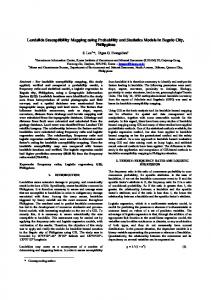
Fig. 1. Statistical probability and mathematical probability

probability may lead students to conceive of probability as being the result of computation, which may hamper students’ understanding about the relation between probability and real-life situations (see [15], [16]). For this reason, emphasizing the dynamics of the relation between statistical probability and mathematical probability through tables and diagrams which depict the converging nature from statistical probability to mathematical probability and revisiting the similarities and differences between these two types of probabilities constantly throughout the probability and statistics unit would help enhance students’ understanding of the concept and its real-life applications ([17], [18], [19]). To this end, this paper provides a class activity using

2.

A c tiv i ty

fo r

Ce n tr a l

L im it

T h eo r e m

 , the The central limit theorem in general tells us that 

mean of a sample generated from a sufficiently large number of iterations of independent random variables, will follow a normal distribution when the sample size is large enough ([20]). Most textbooks introduce and explain this theorem, but rarely provide data that students can visually make sense of. Students can observe how this theorem can be  be the visually understood using Excel. For example, let 

mean of numbers of a die when it is tossed 100 times (which will create a sample consisting of 100 numbers), and then  by create more samples and thus generate several 

iterating 500 tosses. Such results can be cumulated and

Excel.

represented as a discrete graph (Fig 2) or as a continuous  as a simple graph (Fig 3). Fig 2 represents 100 values of 

mean of a set consisting of 100 numbers. In Fig 3, P II.

D E SI GN

OF

TH E

AC T IV IT Y

represents the number of tosses, and N represents the number of samples consisting of P numbers.

1.

A c tiv i ty

fo r

th e

L aw

of

Large

N um b er

The law of large numbers explains the relation between probability and real-life situations, but it can be difficult for students to understand because it involves the concept of the limit. The following activity applies the law of large numbers to die toss. Through this activity, students will experience the law of large numbers by observing how the statistical probability of rolling the number 1 on a die approaches mathematical probability (1/6) when the number of trials is large enough. As shown in Fig 1, students can set the number of rolls of the dice, P. Then, by clicking the button “rolling a die P times,” they toss a die P times. They will observe the

Fig. 2. Distribution of sample mean, when P=100, N=100

Students can easily observe that a discrete variable shown in Fig 2 follows a normal distribution as the number  increases from 30 to 300, to 1000, of times generating 

Re-exploring teaching and learning of probability and statistics using Excel

87

and to a large enough number. All these processes happen

this end, we developed a problem(shown Table 1)and class

simultaneously when the results in Fig 1 are found. In other

material(shown in Fig4).

words, students will observe all these results on one Excel sheet in real time. It shows the dynamics of the graph that

Table 1. Problem statements used in the activity Statement

 found by pushing a button (i. e., Shift + reflects each 

N in Fig 3) rather than showing the results while omitting the process. Such continuous visualizations without omitting

Problem

the intermediate steps in the converging process can provide students a better understanding of the dynamic aspect of the central limit theorem. Specifically, emphasizing the dynamic aspect of the theorem that shows the relation between statistical probability and mathematical probability

Extended problem 1

via its visualization (as P is fixed and N increases, the graph approaches a normal curve as shown in Fig 3) can help various types of students understand the theorem, and also the concept of probability in general.

Extended problem 2

At a company that produces batteries, the probability of making failed product is 10%. If they produce 1000 batteries today, what is the probability of producing greater than equal to 90 failed products and less than equal to 105 failed products?). When the same company produces 1000 batteries, find the probability of making greater than or equal to a failed product, and less than equal to “b” products. Now let’s change the values of “a” and “b”, then find a mathematical probability, and then check how close it is to the statistical probability.). At the same company, let’s change the number of batteries that they produce and the probability of making a failed product. Is statistical probability still similar to the mathematical probability?).

In these data, after students compute the probability based on the assumption that the binomial distribution follows the normal distribution as the number of sample means is large enough, they see that the statistical probability and mathematical probability computed are similar. Thus, they can see that they can assume that the binomial distribution follows a normal distribution and the probability that they found from the data as shown in Fig Fig. 3. As N is increasing, graph-shapes approach to a normal distribution 3.

C o n n e ct io n

di s tr i b uti o n

b e tw e e n

an d

n o r m al

th e

4 is similar to the mathematical probability.

b in o m ia l

d is t r ib ut io n

In probability and statistics, students tend to spend a considerable amount of time solving problems involving a normal distribution curve. They also learn about binomial distribution, which is discrete probability distribution, and then normal distribution, which is a continuous probability distribution. Then, when a random variable X is binomially distributed, its probability is similar to normal distribution when “n” (i. e., number of trials) is large enough. In other words, the key is that X that follows the binomial distribution becomes similar to the normal distribution. However, there is not much class material that visualizes this process. Thus,

Fig. 4. A program for understanding the similarities and differences between statistical probability and mathematical probability

students seem to conceive of it only numerically and then

The main idea of the program shown in Fig 4 is as follows.

just focus on computation by following guided procedures

First, the failure rate for new batteries that the company

and algorithms. Even if they learn the similarities and

produces is the simplest fraction representing probability.

differences between statistical probability and mathematical

Then the program generates random numbers from 1 to the

probability in the beginning of the probability and statistics

denominator of the fraction and these generating processes

unit, their understanding might be limited in terms of

are as many as the number of the batteries that the company

appreciating the use/meaning of statistical probability. To

produces. For example, if the failure rate for new products

88

Journal of The Korea Society of Computer and Information

is 4/13, the program can generate random numbers from 1

enter the number right next to “the trial number” N, and

to 13 as many as the number of batteries that the company

click “find a trial N at once.” For example, Fig 6 shows a

produces. Then, among all these generated random

case of N = 1000. It shows the process of generating

numbers, the way of counting numbers from 1 through the

1000 random numbers and counting the number of failed

numerator 4 (except 5 through 13) reflects the probability

batteries from N equals 1, 2, …, 1000. The fifth column

of producing failed products given the problem. In the case

shows the frequency of the failed battery whose number

presented in Fig 4, the failure rate for new products was

was between 90 and 105, and the sixth column shows the

1/10, so the generated random numbers 1 through 10 were

statistical probability of such cases.

recorded on the first column, and among those generated numbers, 1 would be the number of failed products produced. To apply this idea, first enter the number of batteries produced, the failure rate for new products (denominator “p” and numerator “q”), and the interval for failed products, and generate random numbers as many as the number of batteries produced by clicking the “Number of batteries produced” button(Fig 5). Then, when one clicks the “Number of failed batteries” button, the program counts numbers that represent failed products among random numbers, and records the number(frequency) of such

Fig. 6. A result, when N=1000

numbers in the second column. The process so far is

Fig 6 also includes mathematical probability computed

considered as one trial. If one clicks the “Number of failed

from a normal distribution table. Here, because the total

batteries” but to “n”multiple times, the program repeats the

number of the batteries produced was 1000, the failure rate

trial, and records the number of failed products from each

for new batteries was 1/10, if one lets X be the number of

trial in the third column. Then, the frequencies of such

failed batteries, X ∼ B(1000, 1/10), and thus E(X) = 100

numbers are recorded in the fourth column. For example,

   ). Based on this and Var(X) = 90. Thus, X ∼ N(100, 

Fig5 shows the case when one clicked “Number of failed

information, one can find the mathematical probability, P(90

batteries” five times. For these trials, the numbers of failed

≦X≦105) using the normal distribution function in Excel,

batteries were 119, 98, 80, 125, and 120 in turn. Thus, the

which is recorded in the 13th row. The value of the

frequency of each of those numbers, shown in the fourth

mathematical probability will change depending on the

column, increased to 1 in the fifth column. Because among

number of trials, the failure rate for products, q/p, and the

these five trials, there was one case(i. e., 98) between 90

minimum and maximum for the interval of failed products.

and 105, the statistical probability asked in problem1

Then, the statistical probability can be found by repeating

became 1/5.

the process of generating 1000 random numbers and counting the number of failed products, once, twice … to one thousand times. Thus, students can find the statistical probability for making failed products. Fig7 shows the details of this process.

Fig. 5. Mid-process of the program

Because 5 was the small number, one can also increase the number of trials. To increase the number of trials,

Fig. 7. Statistical probability and mathematical probability using a normal distribution

Re-exploring teaching and learning of probability and statistics using Excel

89

In Fig 7, which shows that |statistical probability -

distribution curve is drawn below them(see Fig 9). We

mathematical probability| is almost 0, one can find that

can input a value referring to reliability α into cell L[2].

the mathematical probability computed from the normal

Then the boundary values belonging to a confidence

distribution table is valid, and the value computed by

 are placed in interval computed from sample mean 

approximating

normal

cells M and N. For instance, the values in M[2] and N[2]

distribution is also valid. Thus, the purpose of this

  . In other words, two are computed from sample mean 

the

binomial

distribution

to

designed program can be effectively attained. Students can

see

that

|statistical

probability-mathematical

probability| is very close to 0, but not zero. Through this “almost zero” value, students may conceive of the importance and meaning of mathematical fact, and by

  

 

         values  ×  



  

 

         and  ×  



     and are computed with the sample probability 

then entered into M[2] and N[2] respectively.

emphasizing that “almost zero” is not zero, students can think of the statistical theory as an approximation of reality, not as reality itself. Furthermore, because one can enter different values in “the number of batteries produced,” “the failure rate for products (denominator “p" and numerator "q"),” and the minimum and maximum of failed products, one can apply this activity to various situations including extended problems 1 and 2. For example, in the case of extended problem 1, one can let "a" be the minimum number of failed products and "b" be the maximum number of failed products of the given interval. Fig. 8. Statistical estimation 4.

S ta tis tic al

e s t im at io n

It is well known that statistical estimation is such a difficult

concept

that

students

mechanically

The reason to use multiplication by n instead of simply

apply

using population mean is because it is more intuitive to

predetermined formulae in solving problems ([21]). In

use sample mean for students than to use population

addition, there is a lack of opportunities for students to

mean. If this method is repeated and then computed

use statistical estimation in a meaningful way. However,

values are entered into cells M[k] and N[k] where 1 ≤ k

statistical estimation is applied to a great deal of real-life

≤ n, the n numbers of M and N cells are represented with

data such as public opinion polls and election predictions.

their boundary values. In these processes, if an expected

Knowing how to determine whether these data are

value E(x) belongs to the confidence interval, the symbol

reliable and how they are modeled mathematically can

O is presented in column O, and if not, the symbol X is

help students to interpret and comprehend diverse social

presented. Finally, the ratio of the symbol O to the total,

phenomena through the mathematical modeling process.

namely, the ratio to measure amount of confidence

Considering modeling as a key process, we developed a

intervals to which the population mean belongs out of a

classroom exercise using Excel to estimate the population

string of n sample means, is presented in cell P[2] in Fig

mean and standard deviation by using a sample mean

8. This value is a meaningful one to show reliability. All

computed from a collection of data out of the population

these processes are represented on a normal distribution

through sampling.

curve for students to visually see and intuitively

In the developed material, which will be applied to diverse

situations

as

a

meaning-making

tool,

the

understand, as shown in Fig 9. If the processes are continuously represented on a normal distribution curve,

population mean and standard deviation acquired from the

students can

trials "n" and "p" are presented in column G and row 17(i.

through visualization. In addition, they can experience the

e., G[17]) and column H and row 17(i. e., H[17])

meaningfulness of statistical estimation because all data

respectively(see Fig 8). In addition, a related normal

inputs as variables can be arbitrarily created and

experience the continuity of thinking

90

Journal of The Korea Society of Computer and Information

manipulated.

and (b) mathematical models that explain reality can have their limitations in general. With this in mind, emphasizing the importance of understanding and reducing the difference between reality and theory becomes an overarching goal for teaching and learning statistics. Based on this conclusion, we can also discuss the use of technology in general. Use of technology can promote a dynamic learning environment where communication among learners and between teachers and students is

Fig. 9. Statistical estimation by 95% confidence interval

considered part of the learning process. In other words, using technology in teaching and learning mathematics can motivate the interest of students, promote student participation in class, and eventually help the class become a dynamic environment where the communication

I I I.

C O NC L U S IO N

between

With the activity introduced in this paper that emphasizes the similarities and differences between statistical probability, mathematical probability through their converging relations, and statistical estimation, we conclude the followings. First, students can have a deeper understanding about probability by experiencing the similarities and differences between statistical probability and mathematical probability with the visual instrument that shows the dynamic processes between the two ([1]). The data including tables and graphs visualized through technology can accommodate student preference in learning tools and thus help their mathematical reflection. Specifically, observing dynamics in which the graphs approach a normal curve would help them understand the concept that probability results from continuous change in variables

in

various

cases,

not

just

as

a

fixed

mathematical probability. Thus, this program can give students a more holistic understanding of probability and statistics in general. Eventually, it positively impacts on students’ interest and attitudes in their mathematical learning ([13], [14]). Second, students can revisit the mathematical meaning of probability through the relationship between binomial distribution, normal distribution, and statistical estimation. Through the program introduced in this paper, students can observe that the difference between statistical probability and mathematical probability is almost zero, but not zero, and can then speculate and explain the reason by examining the data. This experience can help students understand that (a) the meaning of probability and statistical theory as well as its limitation that it cannot be exactly the same as what happens in reality,

teacher

and

students

can

naturally

and

frequently happen ([22], [23]). Second, the activity that involves various representations and cases helps bring the mathematical variability principle and perceptual variability principle ([24]) into the students’ learning process.

Specifically,

representations

through

activities real-time

with

various

technology

help

promote the perceptual variability principle, and including the manipulation of various factors that are included in one mathematical concept while explaining the concept would address the mathematical variability principle. Our conclusions and discussions above provide the following suggestions. First, teachers should understand various aspects of technology, so that they can use it in various teaching and learning situations appropriately. The appropriate use of technology to promote students’ understanding about mathematical concepts and motivate their learning depends significantly on when and how teachers incorporate the technology in their classes. For example, using a graphing calculator in a class where the goal is to learn computation (e. g., for finding the derivative using the definition) may not help teachers achieve that goal. Similarly, teachers’ decisions about how they address mathematical concepts with or without technology would be crucial to maximize the effect of their teaching method in student learning ([8], [25]). Second, curriculum developers and policy makers may need to provide concrete and realistic principles for the use of technology in teaching and learning. Many textbooks provide a fixed picture as an example of using technology. With such pictures students may not visualize the dynamics that technology can provide but conceive of it as one of the representations that textbooks provide

Re-exploring teaching and learning of probability and statistics using Excel

such as a diagram. Activities in which students can

Technology-supported

manipulate numbers and variables may help the class

environments, Reston, VA: NCTM, pp. 165-173, 2005.

become

a

place

mathematical

where

ideas

students

and

thus

can

experience

promote

deeper

understanding of the concepts. Third, we need to develop

mathematics

91

learning

[8] National Council of Teachers of Mathematics. "Principles and standards for school mathematics," Reston, VA: NCTM, 2000.

more activities and materials by which students can gain

[9] D. Lee, "Application of excel on statistics education,"

a deeper understanding of mathematical concepts through

Hong-ik University of the graduate school of education

the use of technology. Providing various representations

master's thesis, 2005.

through technology is important, but developing activities

[10] M. Lee, "A study on teaching high school statistics with

with which students can experience how advanced and

excel," Dankook University of the graduate school of

difficult mathematical concepts are defined and work

education master's thesis, 2010.

would help teachers and students even more in the long

[11] J. Lee, "Studying on education of probability and statistics

run. In this study, we developed a classroom exercise

by using excel," Yonsei University of the graduate school

using Excel to explore how to improve probability and

of education master's thesis, 2007.

statistics

education,

but

we

did

not

verify

its

[12] A. Graham, and M. Thomas, “Representational versatility

effectiveness. It is needed to the effectiveness of the

in learning statistics," International Journal for

developed material and its applicability to educational

Technology in Mathematics Education, vol. 12, pp. 3-14,

contexts.

July 2005. [13] Y. Kim, "A study on teaching and learning probability and statistics education using excel," Ajou University of the graduate school of education master's thesis, 2005. RE F E RE NC E S

[14] M. Lee, "Studying on education of probability and

[1] B. Shin, and K. Lee, "A Study on the Statistical Probability Instruction through Computer Simulation," Journal of Educational Research in Mathematics, vol. 16, no. 2, pp. 139-156. May 2006. [2] L. S. Vygotsky, "Thought and language," Cambridge, MA: MIT Press, 1986. [3] J. Kilpatrick, J. Swafford, and B. Findell, "Adding It Up: Helping Children Learn Mathematics," Washington, DC: National Academies Press, 2001. [4] K. Chang, "Visual Representations and Visual Thinking in Mathematics Education," Journal of the Korea Society of Educational Studies in Mathematics, vol. 2, no. 2, pp. 53-63, December 1992. [5] H. Lew, and J. Lee, "Visualization in Mathematics Education and LoGo," Journal of the Korea Society of Educational Studies in Mathematics, vol. 3, no. 1, pp. 75-85, July 1993. [6] H. Seo, S. Kang, and H. Lim, "The Application of Excel to Probability and Statistics Teaching," Communications of Mathematical Education, vol. 9, pp. 299-316, July 1999. [7] R. C. Caulfield, P. E. Smith, and K. McCormick, "The spreadsheet: A vehicle for connecting proportional reasoning to the real world in a middle school classroom," In

W.

Masalski,

&

P.

C.

Elliott(Eds.),

statistics by using microsoft excel," Kangwon National University of the graduate school of education master's thesis, 2008. [15] D. Nolan, and D. Temple Lang, “Dynamic interactive documents

for

teaching

statistical

practice,"

International Statistical Review, vol. 75, pp. 295-321, December 2007. [16] C. Schwartz, “Computer-aided statistical instruction: multimediocre techno-trash?," International Statistical Review, vol. 75, pp. 348-364, December 2007. [17] S. Lewis, "Laptops in the middle school mathematics classroom," In W. Masalski, & P. C. Elliott(Eds.), Technology-supported

mathematics

learning

environment, Reston, VA: NCTM, pp. 263-275, 2005. [18] C. S. Parke, "Using spreadsheet software to explore measures of central tendency and variability," In W. Masalski, & P. C. Elliott(Eds.), Technology-supported mathematics learning environments, Reston, VA: NCTM, pp. 175-188, 2005. [19] J. B. Plymouth, "Developing mathematical modelling skills: The role of CAS," The International Journal on Mathematics Education, vol. 34, no. 5, pp. 212-220, 2002. [20] J. Woo, K. Park, K. Park, K. Lee, N. Kim, J. Yim, J.

92

Journal of The Korea Society of Computer and Information

Lee, and M. Kim, "Integral Calculus and Statistics,"

Authors

Seoul: Dongapublishing, 2010.

Seungbeom Lee received the B.S degree

[21] W. Kim, S. Moon, and J. Byun, "Mathematics teachers’

in

knowledge and belief on the high school probability and

the

Department

of

Mathematics

Education from Korea University, Korea,

statistics," The Mathematical Education, vol. 45, no. 4,

in 2013. eungbeom Lee is a Mathematics

pp. 381-406, November 2006.

teacher. He has taught students Mathematics.

[22] P. H. Dunham, and T. P. Dick, "Research on graphing

He worked as a teacher in Bromsgrove International

calculators," The Mathematics Teacher, vol. 87, no. 6,

School from U.K. in Thailand. He was also a teacher at

pp. 440-445, 1994.

Dawon International Middle School in Korea.

[23] M. K. Heid, and M. T. Edwards, "Computer algebra

Jungeun Park

received the B.S. in

systems: Revolution or retrofit for today's mathematics

Mathematics

classrooms?" Theory Into Practice, vol. 40, no. 2, pp.

Education in 2005 from Korea University,

128-136, April 2010.

Korea. Jungeun Park also received M.S. in Mathematics

[24] Z. Dienes, "Building up mathematics," London, UK:

P.

C.

Elliott(Eds.),

Technology-supported

mathematics learning environments, Reston, VA: NCTM, pp. 3-15, 2005.

in

and

2007

M.A.

and

PhD

in

in

Michigan State University, U.S.A.

[25] L. Ball, and K. Stacey, "Teaching Strategies for &

2001

Mathematics Education in 2011 from

Hutchinson Educational Ltd, 1960. Developing Judicious Technology Use," In W. Masalski,

in

Dr. Park joined the faculty of the Department of Mathematics at the University of Central Arkansas in 2011. She is currently an assistant professor in the Department of Mathematical Sciences at the University of

Delaware.

She

is

interested

in

undergraduate

mathematics education for STEM majors, discourse analysis for mathematical teaching and learning, and promoting students' mathematical thinking through the use of technology. Sang-Ho Choi received the B. S. in Education

in

2006

from

Chonbuk

National University and the M. S. in mathematics

education

from

Korea

National University of Education, Korea, in 2013. Mr. Choi is currently a graduate student in the Department

of

Curriculum

&

Instruction,

Korea

University. He is interested in mathematics discourse and technology. Dong-Joong

Kim

received his bachelor’s

degree in mathematics education from Korea University, his master’s degree in mathematics from the University of Georgia, and his doctoral degree in mathematics education from Michigan State University. Dr. Kim is an associate professor in the Department of Mathematics Education at Korea University. His research areas

include

discourse

analysis

and

the

use

of

technologies to promote student engagement in learning mathematics. He seeks to engage his students in a search for

relating

discourse.

mathematics

learning

and

teaching

to