SLAM can be categorized into two groups, i.e. laser-based SLAM and vision-based ...... The g2o (âgeneral graph optimizationâ) provides an open-source C++ ...
REAL-TIME 2D AND 3D SLAM USING RTAB-MAP, GMAPPING, AND CARTOGRAPHER PACKAGES Canberk Suat Gurel
Abstract The problem of simultaneous localization and mapping (SLAM) has been one of the most actively studied problems in the robotics community as localization and map building are two essential tasks required for indoor navigation of an autonomous mobile robot without a prior map. SLAM can be categorized into two groups, i.e. laser-based SLAM and vision-based SLAM based on the type of exteroceptive sensor that is used to identify the objects around the robot. This paper presents results obtained from two laser-based SLAM algorithms, i.e. Gmapping and Cartographer, and one vison-based SLAM algorithm, RTAB-Map. TurtleBot3 Waffle platform, which is a low-cost ROS enabled wheeled mobile robot is used in the experiments. LDS-01 laser rangefinder sensor is used for the two laser-based SLAM algorithms whereas two different RGB-D sensors, Microsoft Kinect and Intel RealSense R200 are used for the vision-based SLAM algorithm. The resulting maps successfully described the layout of the Robotics Realization Laboratory, the venue where the experiments were conducted, and are suitable for indoor navigation of a mobile robot. Key words: SLAM, mobile robots, loop closure, data association, gmapping, cartographer, rtabmap
1|Page
Table of Contents Abstract................................................................................................................................. 1 1.
Introduction .................................................................................................................... 3
2.
Related Work ................................................................................................................. 4
3.
Theory ........................................................................................................................... 5 3.1.
Observation ............................................................................................................ 7
3.2.
Data Association ..................................................................................................... 7
3.3.
Relocalization ......................................................................................................... 7
3.4.
Motion Estimation ................................................................................................... 8
3.5.
Optimization ............................................................................................................ 8
3.5.1.
Key-frame-based Optimization ......................................................................... 8
3.5.2.
Filtering-based Optimization ............................................................................ 8
3.6. 4.
Loop Closure ........................................................................................................ 10
Method ......................................................................................................................... 10 4.1.
Laser-Based SLAM ............................................................................................... 11
4.2.
Vision-Based SLAM .............................................................................................. 16
4.2.1.
Sensor: Microsoft Kinect and RealSense R200.............................................. 17
4.2.2.
Frontend: Motion Estimation .......................................................................... 19
4.2.3.
Backend: Graph Optimization ........................................................................ 21
4.3. Discussion of Drawbacks in RGB-D based Methods and Possible Approaches to alleviate these Drawbacks ............................................................................................... 22
5.
4.3.1.
Trade-off between Frame-rate, Bandwidth, and Visual Odometry Robustness 22
4.3.2.
Limited Measurement Range and Error in Depth Measurements ................... 22
4.3.3.
Effect of Ambient Light and Motion Speed of the Sensor ............................... 23
Results ......................................................................................................................... 24 5.1.
Laser-Based SLAM with Gmapping and Cartographer .......................................... 25
5.1.1.
Gmapping ...................................................................................................... 25
5.1.2.
Cartographer.................................................................................................. 26
5.2.
Visual SLAM with RTAB-Map ............................................................................... 28
5.2.1.
Microsoft Kinect Sensor ................................................................................. 28
5.2.2.
Intel RealSense R200 Sensor ........................................................................ 31
6.
Conclusion ................................................................................................................... 34
7.
References .................................................................................................................. 35
8.
Appendix ...................................................................................................................... 38
2|Page
1. Introduction SLAM (Simultaneous Localization and Mapping) can be defined as exploring and mapping the unknown environment while estimating the pose (i.e. position and orientation) of the robot using the sensors mounted on the robot [1]. The availability of a map of the workspace of a robot is a crucial requirement for the autonomous execution of tasks such as localization, navigation, and planning [2]. Robot manipulators, for example, require a detailed model of their workspace for the generation of collision-free motion planning whereas mobile robots (e.g. wheeled, legged, or aerial) need maps such as occupancy grip map for localization and navigation. The required sensor hardware to implement SLAM can be categorized into two based on which system (i.e. localization or mapping) it is serving for. Typically, a proprioceptive sensor is required to localize the robot and an exteroceptive sensor is required for identifying objects around the robot [3]. Encoders and inertial measurement units (IMU) are typically used for pose estimation [1]. The encoder measures the amount of rotation of the driving wheel, which is then used to calculate the approximate pose of the robot. The estimation error in the calculation is compensated using the inertial information measured by the inertial sensor. The estimated pose is corrected once again with the aid of the environmental information obtained through the exteroceptive sensor (i.e. distance sensor or the camera) used to create the map. The mapping system requires the detection of the distance between the robot and the objects around the robot, based on the preferred SLAM technique this can be implemented with laser rangefinders, monocular vision, stereo vision, and RGB-D cameras [4]. Depth cameras such as RealSense R200, Microsoft Kinect, and Xtion have been widely used to extract the distance information [1]. The pose estimation is an important research field of study in robotics [1]. If the pose of the robot is properly estimated, tasks such as SLAM, which is map building based on the pose, can be undertaken accurately [1]. However, there are two key issues in SLAM: uncertainty of the sensor observation information and maintaining the real-time property to operate in actual environment. There are three main methods that (i.e. often referred as three-SLAM-paradigms) have been proposed to solve the pose estimation problem [5]. The first is known as Extended Kalman Filter (EKF) SLAM, it is historically the earliest method that was proposed to address the pose estimation problem; it is the least popular method due to its limiting computational properties and issues that arise as a result of performing a single linearization only. The second uses a nonparametric statistical filtering technique known as particle filter. This method is popular for online SLAM and provides a perspective on addressing the data 3|Page
association problem in SLAM, which is determining the correspondence between observations of image points fetched from the camera at different times. The third is based on graphical representations, which solves the pose estimation problem through nonlinear sparse optimization methods. At present, the third method is considered the state-of-art method for solving the full SLAM problem. In this project, two laser-based SLAM packages, Gmapping (aka Grid Mapping) and Cartographer, and one vision-based SLAM package, RTAB-Map, are used to generate the 2D and 3D maps of the Robotics Realization Laboratory. Gmapping is an efficient RaoBlackwellized particle filer that learns grid maps from laser range data. In Gmapping, each particle carries an individual map of the environment, the number of particles is reduced by computing an accurate proposal distribution taking into account the movement of the robot and also the most recent observation, consequently the uncertainty about the pose of the robot is drastically reduced [6]. The Cartographer, on the other hand, does not employ a particle filter, instead it runs a pose optimization in order to cope with the accumulation of error [7]. In this report is organized as follows: Section 2 provides an overview of the related work in the literature. Section 3 describes the theory of SLAM. Section 4 describes the methods employed for the laser-based SLAM and visual SLAM implementations. Section 5 presents the results obtained using three different packages used for SLAM: Gmapping, Cartographer, and RTAB-Map. Section 6 concludes the paper with a summary of the accomplishments of the project.
2. Related Work Enders [2] and his colleagues presented a novel mapping system that robustly generates highly accurate three-dimensional maps using only a RGB-D camera sensor, i.e. without the need for other sensors. The RGB-D SLAM algorithm that is presented in their paper generates a volumetric 3D map of the environment that can be used for robot localization, navigation, and path planning. With the availability of low-cost RGB-D cameras (e.g. Microsoft Kinect) the approach that they have presented (named RGB-D SLAM) is applicable to robots from autonomous vacuum cleaners to aerial robots. Their approach is based on the extraction of visual keypoints from the color images while the depth images are used to localize the extracted keypoints in three-dimensional space. They used RANSAC to estimate the transformations between associated keypoints and optimized the pose graph using nonlinear optimization. They proposed the use of a beam-based environment measurement model that allows the evaluation of the quality of image-to-image match estimation; using this quality measure it is possible to reject highly inaccurate estimates, 4|Page
allowing their approach to deal with scenarios requiring robustness. The proposed algorithm is tested on publicly available RGB-D benchmark datasets, the presented results demonstrate that the RGB-D SLAM is capable of dealing with fast camera motions (i.e. robot motions) and feature-poor environments while being fast enough for online applications. The RGB-D SLAM algorithm is made available online [8]. However, although the RGB-D SLAM package is reported to be compatible with ROS Kinetic, all the affords of implementing this algorithm were unsuccessful due to an error
REQUIRED process [rgbdslam-1] has died! reported on Jun 6, 2017 [9] (issue number 60). Some people commented that the abovementioned error is resolved with the previous versions of LINUX operating system and ROS (i.e. Ubuntu 14 and ROS Indigo.) As of today, it appears that there is no solution to this error for the users who use Ubuntu 16.04 and ROS Kinetic.
3. Theory A complete SLAM system performs a number of operations repeatedly. First, a set of new landmarks are detected in the environment, initialized (also referred as new landmark initialization), and inserted into the map [4]. As the robot (i.e. observer) moves to a new location, observations are made and matched with the map landmarks, and this process is referred as data association [4]. In case of a tracking failure, relocalization methods are used for recovery. Then, a prior estimation of the robot motion is obtained, this operation is referred as motion estimation. Next, the estimates of landmark positions and robot pose that best explains the data are isolated, eliminating the inaccurate estimates, this operation is referred as optimization. If a previously mapped portion of the environment is reobserved, the loop closure algorithm is executed. Listing 1 shows the sequence of operations that creates a SLAM system.
5|Page
Input to Listing 1: Initial set of landmarks and initial state of observer Output of Listing 1: SLAM map and robot state at each time instant Repeat 1. Observation 2. Data association if tracking failure is detected then 3. Relocalization 4. Motion estimation 5. Optimization if loop closure is detected then 6. Loop closure correction Listing 1: Sequence of operations in SLAM, adapted from [4]
Figure 1: An example SLAM problem, taken from [4]
Figure 1 shows an example instant of SLAM procedure. At time 𝑘, the true state of the observer is given by 𝑥𝑘 . The observer makes observations 𝑧𝑘,𝑖 , 𝑧𝑘,𝑗 , 𝑧𝑘,𝑝 of static landmarks whose true states are given by 𝑚𝑖 , 𝑚𝑗 , and 𝑚𝑝 , respectively. Let 𝑚𝑞 define the true state of a 6|Page
new landmark discovered during the landmark selection process. Based on the corresponding observation of the new landmark denoted as 𝑧𝑘,𝑞 , the state of the new landmark is initialized and inserted into the map. At time 𝑘 + 1, the observer has moved to a new state 𝑥𝑘+1 under the control input 𝑢𝑘+1 . The observer has been able to reobserve two existing landmarks in the map that were previously defined as 𝑚𝑝 and 𝑚𝑞 . Both the corresponding observations 𝑧𝑘+1,𝑝 , 𝑧𝑘+1 , 𝑞 as well as the control input 𝑢𝑘+1 can be utilized to obtain a prior estimate of the incremental motion of the observer between time 𝑘 and 𝑘 + 1. At time 𝑘 + 𝑛, the observer has travelled within its environment and eventually started revisiting previously mapped regions of the environment, namely landmarks that were previously defined as 𝑚𝑖 and 𝑚𝑗 . As depicted in the example illustrated by Figure 1, the estimate state of the observer might not show a close loop (i.e. notice that the true state is a close loop). In the case of observation of previously mapped landmarks, the loop closure algorithm is executed to correct the state of the observer and the states of landmark in the map.
3.1.
Observation
In the observation operation, a new image is received from the RGB-D camera sensor and features, which can be potential landmarks are extracted [4].
3.2.
Data Association
In the data association operation, the correspondences between observations and landmarks are identified, i.e. matching of uncertain measurements with known tracks. There are a number of different methods (e.g. RANSAC, JCBB, active search, and active matching) used for data association [4]. The Joint Compatibility Branch and Bound (JCBB) [10] method uses the fact that observation prediction errors are correlated with each other and hence calculates the joint probability of any set of correspondences. The active search (i.e. covariance-driven gating) approach projects individual covariance predictions of landmarks into the observation image and limits the observation area based on suitable Mahalanobis distance. Active matching [11], on the other hand, considers the joint distribution and uses information theory to guide which landmarks to measure and when to measure them.
3.3.
Relocalization
Camera (or robot) pose tracking failure may occur when the observer moves too fast, the image received from the camera is distorted, blurry or the camera is obstructed. 7|Page
Relocalization refers to automatically detecting and recovering from tracking failures to preserve the integrity of the map [12]. Tracking failure can be identified by the percentage of unsuccessful observations and large uncertainty in the camera pose [12]. The pose of the camera is recovered by establishing correspondence between the image and the map and solving the resulting perspective pose estimation problem [12].
3.4.
Motion Estimation
The motion of the observer can be predicted based on the odometry information. The odometry information stands as a prior estimate of the observer state and covariance, which is later used in the optimization stage.
3.5.
Optimization
SLAM algorithms typically employ either key-frame-based optimization or filtering-based optimization. For instance, the Gmapping package uses filtering-based optimization (e.g. Rao-Blackwellized Filter) while the RTAB-Map package uses key-frame-based optimization. According a paper [13] published in 2017 (and later revised in 2018), although filter-based monocular SLAM systems were common for the past decade, the more efficient key-framebased solutions are becoming the de facto methodology for building a monocular SLAM system. 3.5.1. Key-frame-based Optimization Key-frame-based optimization splits camera pose tracking and mapping into two separate processes. The accuracy of camera pose estimation is increased by using measurement from large numbers of landmarks per frame. The map is usually estimated by performing bundle adjustment over only a set of frames (i.e. keyframes) since measurements from successive image frames provides redundant and therefore less information for a given computational budget [14]. The kef-frame-based optimization is further covered in Section 4.2. Vision-Based SLAM. 3.5.2. Filtering-based Optimization The SLAM problem requires the computation of joint posterior density pf the landmark locations and observer state at time 𝑘, given the available observations and control inputs up to and including time 𝑘, together with the initial state of the observer [15]. The probability distribution is stated as 𝑃(𝑥𝑘 , 𝑚|𝑍0:𝑘 , 𝑈0:𝑘 , 𝑥0 ) where the terms are defined as 8|Page
𝑥𝑘 : observer state vector,
𝑚: vector of all landmark states, 𝑚𝑖 ,
𝑍0:𝑘 : vector of all landmark observations, 𝑧𝑖,𝑘 ,
𝑈0:𝑘 : vector of all past control inputs, 𝑢𝑘 .
Given an estimate for the problem at time 𝑘 − 1, 𝑃(𝑥𝑘−1 , 𝑚|𝑍0:𝑘−1 , 𝑈0:𝑘−1 , 𝑥0 ) a recursive solution to the problem can be obtained by employing a state transition (i.e. motion) model 𝑃(𝑥𝑘 |𝑥𝑘−1 , 𝑢𝑘 ) and an observation model 𝑃(𝑧𝑘 |𝑥𝑘 , 𝑚), which characterize the effect of the control input and observation, respectively [3]. As a result, the SLAM algorithm can now be expressed as a standard two step recursive prediction (i.e. time update) 𝑃(𝑥𝑘 , 𝑚|𝑍0:𝑘−1 , 𝑈0:𝑘 , 𝑥0 ) = ∫ 𝑃(𝑥𝑘 |𝑥𝑘−1 , 𝑢𝑘 ) 𝑃(𝑥𝑘−1 , 𝑚|𝑍0:𝑘−1 , 𝑈0:𝑘−1 , 𝑥0 ) 𝑑𝑥𝑘−1 and correction (i.e. measurement update) 𝑃(𝑥𝑘 , 𝑚|𝑍0:𝑘 , 𝑈0:𝑘 , 𝑥0 ) =
𝑃(𝑧𝑘 |𝑥𝑘 , 𝑚)𝑃(𝑥𝑘 , 𝑚|𝑍0:𝑘−1 , 𝑈0:𝑘 , 𝑥0 ) 𝑃(𝑧𝑘 |𝑍0:𝑘−1 , 𝑈0:𝑘 )
This is an ongoing process where the time update predicts the state estimate ahead in time and the measurement update modifies this estimate using the actual measurement at that time [3]. Two solution methods to the probabilistic SLAM problem are Extended Kalman Filter (EKF) Based SLAM and Rao-Blackwellized Filter Based SLAM. 3.5.2.1.
EKF Based SLAM
Kalman Filter only applies to linear systems; however, most of the robots and sensors are nonlinear systems that require the nonlinear version of Kalman Filter, Extended Kalman Filter [1]. The general form of the EKF prediction step can be customized for SLAM to minimize the computation time, since there is no need to perform a time update for landmark states 𝑚𝑖 : 𝑖 = 1 … 𝑛, if the landmarks are stationary [15]. Hence only the observer state, 𝑥𝑘 , needs to be predicted ahead and the new error covariance of the predicted observer state needs to be computed [15]. The new time update equations for the covariance items that require an update are as follows. 𝑃𝑥−𝑘+1 𝑥𝑘+1 =
𝜕𝑓𝑣 𝜕𝑓𝑣 𝑇 𝜕𝑓𝑣 𝜕𝑓𝑣 𝑇 𝑃𝑥𝑘 𝑥𝑘 + 𝑃𝑛𝑛 𝜕𝑥𝑘 𝜕𝑥𝑘 𝜕𝑛 𝜕𝑛
𝑃𝑥−𝑘+1 𝑚𝑖 =
𝜕𝑓𝑣 𝑃 𝜕𝑥𝑘 𝑥𝑘 𝑚𝑖
9|Page
where the terms are defined as
{∙}− : time update estimate,
𝑛: noise in the observer motion model,
𝑃𝑛𝑛 : noise covariance of the observer motion model,
− 𝑓𝑣 : observer state transfer function 𝑥𝑘+1 = 𝑓𝑣 (𝑥𝑘 , 𝑛) such that 𝑥𝑘+1 = 𝑓𝑣 (𝑥𝑘 , 0).
The computational complexity of the EKF-SLAM solution grows quadratically with the number of landmarks due to the calculations involved in the EKF update steps [4]. 3.5.2.2.
Rao-Blackwellized Filter Based SLAM
Rao-Blackwellized Filter based SLAM algorithms operate based on the following principle: given the observer trajectory, which assumed to be correct, then different landmark measurements are independent of each other. Hence a particle filter can be used to estimate the trajectory of the observer, each particle carrying an individual map of the environment. Since landmarks within this map are independent, each landmark can be represented with low-dimensional EKF. As a result, Rao-Blackwellized filter based SLAM has linear complexity rather than quadratic complexity as in EKF based SLAM.
3.6.
Loop Closure
Ideally when previously mapped regions of an environment are reobserved, the SLAM algorithm should recognize the corresponding landmarks in the map; however, particularly in long trajectory loops, such as the Robot Realization Laboratory, landmark states in two corresponding regions of the map can be incompatible given the uncertainty in estimates. To overcome this issue, loop closure methods (e.g. image-to-image matching [16], image-tomap matching [17], and hybrid methods [18]) are utilized to align the corresponding regions of the map, making it globally coherent.
4. Method Robot localization is informed by measurements of range and positions of the landmarks located within the workspace. Sensors that measure range can be based on different principles, for instance, laser rangefinders, ultrasonic rangefinders, computer vision or radar can be used to measure the distance between the robot and a landmark. Laser rangefinders provide only a linear cross section of the world, rather than an area as a camera does [19]. This is ideal when the goal is to generate the occupancy grid of an area that can later be used for navigation purposes. However, if the goal is to create a 3D-map then a RGB-D camera needs to be installed. In this project, both laser-based SLAM (using
10 | P a g e
the LDS-01 sensor) and visual-based SLAM (using Kinect and R200 sensors) are implemented. As the robot platform a ROS enabled mobile robot, TurtleBot3 was chosen. The core technologies of TurtleBot3 are SLAM, navigation, and manipulation, making it suitable for this project.
4.1.
Laser-Based SLAM
TurtleBot3 is equipped with a 360 Laser Distance Sensor (LDS-01) that is a 2D laser scanner capable of scanning 360 degrees with the aid of a DC motor that is attached to the sensor by a rubber belt drive. The laser rangefinder emits short pulses of infra-red laser light and measures how long it takes for the reflected pulse to return [19]. The time-of-flight is used to calculate the distance. Figure 2 shows the LDS-01 LIDAR sensor; the distance range is between 12cm and 350cm whereas the sampling rate is 1.8 kHz [20].
Figure 2: LDS-01 LIDAR sensor, adapted from [20]
If the pose of the mobile robot is sufficiently well known through the onboard IMU or alternatively using the wheel encoders, then the laser scans can be transformed into global coordinate frame, which then can be used to build a map by employing a probabilistic approach. For a robot at a given pose, each range measurement in the scan determines the coordinates of a cell that contains an obstacle however the robot has no information about the cells that are behind the detected obstacles, these cells are registered as unknown cells whereas the cells that are between the sensor and the detected obstacles are registered as obstacle-free cells. The maximum distance of LDS-01 rangefinder (i.e. 350cm) plays a key role in the measurements, if there is no returning laser pulse within 23.33ns then the robot registers all the cells within 350cm range in the direction of emitted laser pulse as obstaclefree cells [19]. Figure 3 is provided as an example of how the laser rangefinder operates. In this example, the grid cell size of 5cm is chosen, the sensor is located at cell (0,0), 17 rays are emitted while an area of 79.7° is scanned. The unexplored and the unknown cells that
11 | P a g e
are behind the obstacle are shown by gray whereas white cells are the obstacle-free cells and the black cells are the occupied cells.
Figure 3: Laser scan about cell (0,0). White, gray and black indicate obstacle-free, unknown, and occupied cells, respectively. Blue lines indicate the laser beams.
Now that a diagonal obstacle is detected, a line can be fitted to analytically express the obstacle. Least Squares Estimation (LSE) is used to fit a line to the obtained data points. Figure 4 shows the result of the line fitting procedure.
12 | P a g e
Figure 4: Line fitting using LSE
The estimated wall is defined by the equation 𝑦 = 0.6379 − 1.2415𝑥
Equation 1
However, the equation of the line that is fitted to the obstacle is not useful unless we relate it to the robot. In order to relate the line to the robot the normal line needs to be calculated. Let us define the line in polar coordinates 𝑚𝐴𝑅 = (𝛼, 𝑟) at the point which is normal to the line. The normal line is shown by Figure 5.
13 | P a g e
Figure 5: Normal line and the fitted line
If two points 𝐴 and 𝐵 with coordinates (𝑥1 , 𝑦1 ) and (𝑥2 , 𝑦2 ) are identified on the line that was previously defined by Equation 1, the polar coordinates (𝜃1 , 𝑑1 ) and (𝜃2 , 𝑑2 ) can be computed by Equations 2 and 3. 𝑦𝑖 𝜃𝑖 = 𝑎𝑡𝑎𝑛2 ( ) 𝑥𝑖
Equation 2
𝑑𝑖 = √𝑥𝑖 2 + 𝑦𝑖 2
Equation 3
To calculate the polar coordinates 𝑚𝐴𝑅 of the normal line, the following relationships are used 𝜎𝑑1 𝑑2 sin(𝜃1 − 𝜃2 )
𝑟=
√𝑑1 2 + 𝑑2 2 − 2𝑑1 𝑑2 cos(𝜃1 − 𝜃2 )
𝛼 = cos −1
𝜎(𝑑2 sin(𝜃2 ) − 𝑑1 sin(𝜃1 )) 2 √ 2 ) ( 𝑑1 + 𝑑2 − 2𝑑1 𝑑2 cos(𝜃1 − 𝜃2 )
where 14 | P a g e
𝜎 = 𝑠𝑖𝑔𝑛(sin(𝜃1 − 𝜃2 )) The polar coordinates of the normal line is calculated as 𝑚𝐴𝑅 = (38.9°, 0.4). Unfortunately, there is rarely a single wall to be identified, often there are lots of unconnected lines which need to be separately identified. The LSE method is not applicable to this kind of scenarios. There are a number of different line extraction algorithms which have been designed to deal with complex environments. Table 1 shows the comparison of some of the commonly used line extraction algorithms.
Table 1: Comparison of line extraction algorithms, taken from [21]
The line extraction algorithm that is used in both 2D SLAM packages, Gmapping and Cartographer, used is the split-and-merge algorithm. The procedure of the algorithm is illustrated by Figure 6. The line estimation is done using LSE where the first and last data points are connected by a straight-line. Then a normal line is found that connects the furthest data point to the straight line between the first and the last data points. If the length of the normal line is greater than a given threshold, the line splits into two, connecting the first and last data points with the furthest data point. This procedure is repeated until the length of the normal line is less than the pre-defined threshold value.
Figure 6: Split-and-merge algorithm procedure
15 | P a g e
The split-and-merge algorithm is applied to data points obtained from LIDAR. The line extraction algorithm has successfully identified 5 walls. Figure 7 shows the obtained results.
Figure 7: Lidar data points (in blue) and the lines obtained from the split-and-merge algorithm
4.2.
Vision-Based SLAM
Visual SLAM can be defined as the problem of building maps and tracking the robot pose in full 6-DOF using data from cameras (i.e. RGB-D sensors). RGB-D sensors offer the visual information that enables the construction of rich 3-D models of the world [5]. They also enable difficult issues such as loop-closing to be addressed in novel ways using appearance information [5]. RTAB-Map (Real-Time Appearance-Based Mapping) is a RGB-D graph-based SLAM approach based on an incremental appearance-based loop closure detector [22]. Loop closure is the problem of recognizing a previously-visited location and updating beliefs accordingly. The loop closure detector uses a bag-of-words approach to determinate how likely a new image comes from a previous location or a new location. When a loop closure 16 | P a g e
hypothesis is accepted, a new constraint is added to the map’s graph, then a graph optimizer minimizes the errors in the map. A memory management approach [23] is used to limit the number of locations used for loop closure detection and graph optimization, so that real-time constraints on large-scale environments are always respected. A graph-based SLAM system such as RTAB-Map consists of three stages: sensor measurement, frontend, and backend. In the frontend stage, the sensor data is processed and the geometric constraints between the successive RGB-D frames are extracted. While the odometry was estimated in the frontend stage, the backend stage is focused on solving the accumulated drift problem and on detecting the loop closure in Loop Detection. Finally, the 3D map is generated by using the g2o algorithm in Global Optimization. Figure 8 illustrates the flowchart of the proposed method.
Figure 8: Stages of the Real-Time Appearance-based Mapping (RTAB-Map), adapted from [24]
4.2.1. Sensor: Microsoft Kinect and RealSense R200 RGB-D camera sensors such as Microsoft Kinect and RealSense R200 are alternatives to laser range scanners that make visual SLAM possible. Both sensors are equipped with IR emitters that project structured light in the infrared spectrum, the reflected light is perceived by infrared camera(s) with a known baseline. In Kinect sensor, the disparity between the projected pattern and the pattern observed by the infrared camera is used to compute the depth information by triangulation using the known baseline. The R200 sensor, on the other hand, has two IR cameras, allowing the sensor to make use of stereoscopy photography to 17 | P a g e
calculate the depth from the disparity between the 2 separate cameras using triangulation. Figure 9 shows the Kinect and R200 sensors.
Figure 9: (a.) Microsoft Kinect sensor, (b.) Intel RealSense R200 sensor, (c.) internals of the Microsoft Kinect sensor, and (d.) internals of the Intel RealSense R200 sensor
Table 2 shows the comparison of the two sensors that are used to create the 3D map of the Robot Realization Lab (RRL). Microsoft Kinect
RealSense R200
Depth Resolution (px)
640 x 480
640 x 480
RGB Video Resolution (px)
1600 x 1200
1920 x 1280
Range (m)
0.5 – 5
0.3 – 4
Frame Rate (fps)
30 (RGB), 60 (IR depth)
30 (RGB), 60 (IR depth)
Diagonal Field of View (deg)
71.4 (RGB)
77 (RGB), 70 (IR depth)
Number of IR camera(s)
1
2
Number of RGB camera(s)
1
1
Table 2: Comparison of Kinect and R200 RGB-D camera sensors
The experiments revealed that since both sensors are using infrared radiation (IR) emitters and infrared cameras to detect the distance, the depth detection performance of both cameras are dependent on the lighting conditions and the reflectivity of the surface. Figures 10 and 11 show the depth and RGB images captured by Microsoft Kinect and RealSense R200 sensors, respectively.
18 | P a g e
Figure 10: Depth Image and RGB image captured by Microsoft Kinect sensor
Figure 11: Depth Image and RGB image captured by RealSense R200 sensor
4.2.2. Frontend: Motion Estimation In the frontend stage, the sensor data is processed to extract the geometric relationships between the robot, i.e. TurtleBot3 and the landmarks located within the environment of the robot. Wheel encoders and IMU sensors that are typically used in laser-based SLAM are capable of measuring the motion itself, however using a RGB-D camera, the motion needs to be computed from a sequence of observations. The process of determining the position and orientation of a robot (i.e. camera) by analyzing the associated camera images is called visual odometry. To find the visual odometry, the most important part is the feature extraction and matching in successive frames. A feature is a small part or region within the image, which differs from the pixels in its proximity. This difference is often described by color and intensity, and the difference is noticed in edges and blobs. At present, there are 19 | P a g e
several feature detection/extraction and match algorithms (e.g. SIFT, SURF, MSER, BRISK) that are available to undertake the visual odometry task; in particular, Speeded Up Robust Features (SURF) algorithm [25] is used in this project. The following steps are taken in order to obtain the transformation estimation 𝑇(𝑥, 𝑦, 𝑧, 𝑟𝑜𝑙𝑙, 𝑝𝑖𝑡𝑐ℎ, 𝑦𝑎𝑤):
Frame 𝑛 and 𝑛 + 1 are converted into gray scale,
The SURF features are detected,
The features (i.e. descriptors) and their corresponding locations are extracted,
Indices of the matching features and the distance between the matching features are found,
The fundamental matrix is found by employing RANSAC to be more robust against false positive matches,
Relative camera orientation and location are found by making use of the inliers in frame 𝑛 and 𝑛 + 1, camera parameters, and the fundamental matrix,
Using the relative orientation and the relative location, the 𝑅𝑜𝑡𝑎𝑡𝑖𝑜𝑛 𝑀𝑎𝑡𝑟𝑖𝑥 and the 𝑇𝑟𝑎𝑛𝑠𝑙𝑎𝑡𝑖𝑜𝑛 𝑉𝑒𝑐𝑡𝑜𝑟 are found.
Then the obtained 𝑅𝑜𝑡𝑎𝑡𝑖𝑜𝑛 𝑀𝑎𝑡𝑟𝑖𝑥 and 𝑇𝑟𝑎𝑛𝑠𝑙𝑎𝑡𝑖𝑜𝑛 𝑉𝑒𝑐𝑡𝑜𝑟 are used to update the current camera pose. Equations 4 and 5 are used to update the camera pose, where 𝑇𝑟𝑎𝑛𝑠 and 𝑅𝑜𝑡 were initially declared as [0; 0; 0] and diag{1,1,1}, respectively. 𝑇𝑟𝑎𝑛𝑠𝑘 = 𝑇𝑟𝑎𝑛𝑠𝑘−1 + 𝑅𝑜𝑡𝑘−1 ∗ 𝑇𝑟𝑎𝑛𝑠𝑙𝑎𝑡𝑖𝑜𝑛 𝑉𝑒𝑐𝑡𝑜𝑟 𝑅𝑜𝑡𝑘 = 𝑅𝑜𝑡𝑘−1 ∗ 𝑅𝑜𝑡𝑎𝑡𝑖𝑜𝑛 𝑀𝑎𝑡𝑟𝑖𝑥
Equation 4 Equation 5
Figures 12 and 13 show the inlier matching points on RGB image, and depth image, respectively.
Figure 12: Inlier matching points on RGB image [24]
20 | P a g e
Figure 13: Inlier matching points on depth image [24]
4.2.3. Backend: Graph Optimization An intrinsic problem of visual odometry is the appearance of drift in the estimated trajectory of the robot. The drift is caused by error accumulation, as visual odometry is based on relative measurements, and will grow unboundedly with distance travelled [26]. The majority of the error is introduced by the uncertainty in the sensor measurements (i.e. sensor noise) and the false positive matches. In order to alleviate the accumulated drift problem, the keyframe technique is applied [27]. The key-frames are selected by the pre-defined parameters. For example, if the correspondence of 3D inliers with respect to the reference key-frame is greater than the threshold, the current frame will be dropped and the next frame will be captured. Until the correspondences of 3D inliers with respect to the reference key-frame is less than the threshold (at least 50 inliers), the rigid transformation is estimated and the current frame is selected as the reference key-frame. In the mapping process, the key-frames are selected by the displacement rather than the correspondences of the 3D inliers. If the displacement of the translation or the rotation with respect to the reference key-frame is larger than the threshold, the current frame is stored in the Loop Detection buffer. While a new key-frame is inserted, it is compared to all previous key-frames in the Loop Detection buffer. If the correspondences of the 3D inliers are more than the threshold between the current key-frame and the previous key-frames in the buffer, it indicates that there is a loop inside the Loop Detection. When a loop is detected, the global poses are optimized by the g2o optimization algorithm [28]. The g2o (“general graph optimization”) provides an open-source C++ framework for optimizing graph-based nonlinear error functions using least squares. It is applied into the Visual SLAM system to obtain a 3D global consistency map.
21 | P a g e
4.3.
Discussion of Drawbacks in RGB-D based Methods and Possible Approaches to alleviate these Drawbacks
RGB-D sensors are novel sensing systems that capture RGB image along with pixel-wise depth information. Although they are widely used in various applications, RGB-D sensors have a number of significant drawbacks including limited frame rate, limited bandwidth for data transmission, limited measurement ranges, and errors in depth measurement. Compared to the laser-based approaches, the depth measurements acquired from RGB-D cameras are much noisier and their field-of-view (~70°) is far more constraint considering that the laser rangefinders have a field-of-view of 360° [29]. Furthermore, illumination of the ambient and motion speed of the camera also play an important role in the performance of the RGB-D sensor. 4.3.1. Trade-off between Frame-rate, Bandwidth, and Visual Odometry Robustness Processing of the visual information obtained by the RGB-D sensor can be computationally exhaustive and hence it is often required to transmit this data to a computer equipped with a dedicated GPU rather than loading this burden on the on-board CPU. However, typically limited bandwidth to send/receive camera frames oblige the frames to be compressed, reducing the resolution and hence making the algorithm unable to resolve small details within the scene. In order to overcome this issue, the frequency of the camera is reduced at the cost of the robustness of visual odometry, which is further covered in Section 5.2.1. Microsoft Kinect Sensor. 4.3.2. Limited Measurement Range and Error in Depth Measurements The 3D scene reconstructed from RGB image sequences is expected to have a larger range compared to the one from the depth sensor, which typically has a range up to 5m. The limited range measurement makes frame matching such a hardship that the motion between frames can only be recovered up to a scale factor, and the errors in tracking motion can accumulate over time during frame-to-frame estimation. The error accumulation issue is addressed by the implementation of a loop closure algorithm, as discussed earlier in Section 3.6 Loop Closure. Tang [30] et al. proposed a novel approach to overcome the range drawback of the RGB-D sensors, their method did not only enlarge the measurement range of RGB-D sensors, but also enhanced scene details that were lack of depth information. In paper [30], Tang [30] et al. introduced an approach for geometric integration of depth scene and RGB scene to enhance the mapping system of RGB-D sensors for detailed 3D modeling of large indoor and outdoor environments. In their approach, first, a precise calibration
22 | P a g e
method is employed to obtain the full set of external and internal parameters as well as the relative pose between RGB camera and IR camera. Second, to ensure poses accuracy of RGB images, a refined false features matches rejection method is introduced by combining the depth information and initial camera poses between frames of the RGB-D sensor [30]. Then, a global optimization model is used to improve the accuracy of the camera pose and to minimize the inconsistencies between the depth frames. The geometric inconsistencies between RGB scene and depth scene are eliminated by integrating the depth and visual information and a robust rigid-transformation recovery method is developed to register RGB scene to depth scene. The feasibility and robustness of the proposed method is proven by conducting experiments on publicly available datasets. Despite the encouraging results presented in their paper, it should be noted that the current implementation of their approach is not real-time. 4.3.3. Effect of Ambient Light and Motion Speed of the Sensor Ambient light plays a vital role on the depth measurement performance of some 3D cameras that use active illumination, e.g. sensors that use structured light [31]. To recap, both Microsoft Kinect and RealSense R200 sensors use structured light; Microsoft Kinect is equipped with a monocular IR camera while RealSense R200 is equipped with stereo IR camera. Creating RGB-D sensors that are immune to the effects of ambient lighting fills a practical need, e.g. outdoor mapping, where the sensor is required to operate under direct exposure of sunlight. Each 3D imaging technology, e.g. time-of-flight, stereovision, fixed structured light, and programmable structured light (DLP) is affected by ambient light in a different way [32]. Stereovision approach does not rely on active illumination and hence it is suitable for outdoor usage, in contrast, structured light relies upon a projected intensity pattern to obtain depth. The pattern can be easily corrupted by ambient light and ambient shadows [32]. Therefore, the depth measurement performance of both of the RGB-D sensors used in the experiments is susceptive to ambient light. In order to alleviate the effect of ambient light, Microsoft Kinect sensor uses an optical filter to reject wavelengths that are not in the active illumination however the sunlight contains a significant amount of near-infrared light, this only help marginally and the sensor is still limited to indoor usage. In the next generation of Microsoft Kinect sensor (aka Kinect v2) time-of-flight technique is used to measure depth, allowing the Kinect v2 sensor to outperform its ancestor in outdoor experiments [31]. However, it is reported that when it is too bright, the imaging sensor saturates and the depth information is lost.
23 | P a g e
The motion speed of the robot effects the accuracy of the depth measurements. Most of the RGB-D sensors including Microsoft Kinect and RealSense R200 utilize a multishot technique where multiple photographs (i.e. subframes) of the scene are taken in order to generate a single depth frame [31]. If there is substantial motion between the subframes, the depth sensing capability is degraded as severe artifacts are seen in the depth frame [31].
5. Results All of the experiments are undertaken in Robotics Realization Laboratory (RRL) where the laboratory is mapped using two different laser-based SLAM packages (i.e. Gmapping and Cartographer) and one visual SLAM package (i.e. RTAB-Map). The RRL is 11.3m wide and 10.33m long room, allowing the trajectory of the robot to be long enough to test how the loop closure algorithm works. Both Kinect and R200 RGB-D sensors are used while creating the 3D map of the laboratory and the obtained results are compared. Figure 14 shows the two robot configurations used for the experiments. The robot on the left (Figure 14 a.) is equipped with the Kinect sensor, R200 sensor, IMU, encoders, and a GoPro while the robot on the right (Figure 14 b.) is equipped with the LDS-01 LIDAR sensor, IMU, encoders, and the R200 sensor. In both of the robots the IMU and encoder combination is used to estimate the pose of the robot while the Kinect and R200 RGB-D sensors are used for visual input (i.e. RGB image and depth image) and the LIDAR sensor is used for distance input.
Figure 14: (a.) the robot configuration used for visual SLAM and (b.) the robot configuration used for laser-based SLAM
24 | P a g e
The maps generated with two laser-based SLAM packages (i.e. Gmapping and Cartographer) and one vision-based SLAM package (i.e. RTAB-Map) are nearly identical, proving accuracy of the obtained results.
5.1.
Laser-Based SLAM with Gmapping and Cartographer
The laser-based SLAM packages that are used in this project proved to have several characteristic constraints. As the LDS-01 LIDAR emits infrared light, the objects that are matte-black (e.g. in RRL trash bins are matte-black), glasses that do not reflect infrared light (e.g. TV and monitor displays), and mirrors that scatter light (e.g. white boards in RRL have a similar effect) degraded the SLAM performance of the tested laser-based SLAM packages, i.e. Gmapping and Cartographer. It is also well known that long corridors without any distinctive obstacles, square-shaped rooms and open wide areas where no obstacle information can be acquired make the laser-based SLAM algorithms nonoperational [1]. One of the difficulties faced while mapping the RRL using the Gmapping and Cartographer packages was the power consumption. The onboard LiPo battery is an 1800mAh 11.1V battery, which lasts approximately 15-20 minutes depending on how fast the robot is driven. If the mapping is not completed within this period of time, the incomplete map can be saved but it cannot be completed by replacing the battery, i.e. the mapping needs to be redone from scratch. 5.1.1. Gmapping Gmapping is the built-in SLAM package. The following steps needs to be taken to execute SLAM using the Gmapping package. i.
[Remote PC] Run roscore.
$ roscore ii.
[TurtleBot] Bring up basic packages to start TurtleBot3 applications.
$ roslaunch turtlebot3_bringup turtlebot3_robot.launch iii.
[Remote PC] Open a new terminal and launch the SLAM file.
$ export TURTLEBOT3_MODEL=roscore $ roslaunch turtlebot3_slam turtlebot3_slam.launch slam_methods:=gmapping
iv.
[Remote PC] Open a new terminal and run the teleoperation node.
$ export TURTLEBOT3_MODEL=waffle $ roslaunch turtlebot3_teleop turtlebot3_teleop_key.launch
25 | P a g e
v.
[Remote PC] Save the generated map.
$ rosrun map_server map_saver -f ~/map Figure 15 shows the generated map of RRL using the Gmapping SLAM package. The 2D maps provide only a cross-section of the room, considering that the robot height is only 14.1cm (see Figure 23 in Appendix), the pixelated black dots in Figure 4.14 actually are the legs of desks and chairs in RRL, i.e. they are not errors. It can be seen that the left top of the map is in complete, this is where the previously mentioned matte-black trash bin was located and hence the algorithm has no information about that part of the room.
Figure 15: The 2D map of RRL generated with Gmapping
5.1.2. Cartographer The Cartographer package does not come pre-installed and the Cartographer dependency packages can be installed as follows:
26 | P a g e
$ sudo apt-get install ninja-build libceres-dev libprotobuf-dev protobufcompiler libprotoc-dev $ cd ~/catkin_ws/src $ git clone https://github.com/googlecartographer/cartographer.git $ git clone https://github.com/googlecartographer/cartographer_ros.git $ cd ~/catkin_ws $ src/cartographer/scripts/install_proto3.sh $ rm -rf protobuf/ $ rosdep install --from-paths src --ignore-src -r -y --os=ubuntu:xenial $ catkin_make_isolated --install --use-ninja
The steps taken for the execution of the Gmapping package applies to Cartographer package except step iii. needs to be replaced by
$ export TURTLEBOT3_MODEL=waffle $ source ~/catkin_ws/install_isolated/setup.bash $ roslaunch turtlebot3_slam turtlebot3_slam.launch slam_methods:=cartographer Figure 16 shows the generated map of RRL using the Cartographer SLAM package. If compared to the map generated by Gmapping package, it can be seen that the results are nearly identical except that the Cartographer package did a slightly better job at the left top corner of the map.
Figure 16: The 2D map of RRL generated with Cartographer
27 | P a g e
5.2.
Visual SLAM with RTAB-Map
The RTAB-Map package provides a graphical user interface named as rtabmapviz, which visualizes visual odometry, output of the loop closure detector, and a point cloud that is a 3D dense map. The generated map can be saved in PLY and PCD formats and can be visualized using the MeshLab software. The results obtained using Microsoft Kinect and Intel RealSense R200 sensors are as follows. 5.2.1. Microsoft Kinect Sensor Using the Kinect sensor, the generated 3D map was denser and the quality was better compared to the one generated using the RealSense R200 sensor. The number of outlier was small due to the used filtering method and the number of inliers were always high enough to obtain an uninterrupted visual odometry with an average deviation of 37 cm. One drawback of using the Kinect sensor was that the sensor needs to be powered by an external power supply, and hence a 12V regulator circuit [33] needed to be made. Since this process requires the splitter cable to be permanently damaged, a very long extension cord is used to supply power to the robot. Another hardship that was faced was to do with the speed of the image stream over Wi-Fi. This problem causes the map building process to be very slow, eventually leading the software to crash. This issue is resolved by throttling the messages received from Kinect sensor to 5 Hz in order to reduce the bandwidth used on the Wi-Fi network. Consequently, the bandwidth requirement is reduced down to approximately 500 KiB/s. Figure 17 shows the 3D cloud map of one section of the RRL where the image on the left bottom is taken by a DSLR camera for comparison purposes.
28 | P a g e
Figure 17: 3D point cloud of the RRL where the Baxter and Sawyer robots are located.
The same experiment is repeated and Figure 18 shows obtained result. In this experiment, instead of driving around the Baxter and Sawyer robots, the TurtleBot3 remained stable. It can be seen that the window that is located behind the Baxter robot did not reflect the infrared light emitted by the Kinect sensor and hence that regions is marked black, i.e. unknown area.
Figure 18: 3D point cloud of Baxter and Sawyer robots by keeping the camera position stable.
29 | P a g e
Figure 19 shows the 3D map of the entire laboratory where the blue line shows the odometry of the camera obtained by the visual odometry. The resulting map successfully describes the layout of the laboratory.
Figure 19: 3D map of the entire laboratory
The following steps needs to be taken to execute SLAM using the RTAB-Map package with Kinect sensor. i.
[Remote PC] Install RTAB-Map to PC.
$ sudo apt-get install ros-kinetic-rtabmap-ros
ii.
[TurtleBot] Install RTAB-Map to TurtleBot3.
$ sudo apt-get install ros-kinetic-rtabmap-ros
iii.
Create a file called freenect_throttle.launch inside the TurtleBot3 and copy/paste the code that is provided in the Appendix (Listing 2).
iv.
[Remote PC] Run roscore.
30 | P a g e
$ roscore v.
Connect the Microsoft Kinect sensor to the robot and [TurtleBot] run the turtlebot3_bringup node
$ roslaunch turtlebot3_bringup turtlebot3_robot.launch
vi.
[TurtleBot] Launch the freenect_throttle.launch file running the following command
$ roslaunch freenect_throttle.launch rate:=5
vii.
[Remote PC] Launch rtabmapviz graphical user interface
$ roslaunch rtabmap_ros rtabmap.launch rgb_topic:=/camera/data_throttled_image depth_topic:=/camera/data_throttled_image_depth camera_info_topic:=/camera/data_throttled_camera_info compressed:=true rtabmap_args:="--delete_db_on_start"
viii.
[Remote PC] Open a new terminal and run the teleoperation node.
$ export TURTLEBOT3_MODEL=waffle $ roslaunch turtlebot3_teleop turtlebot3_teleop_key.launch
ix.
[Remote PC] After the mapping is completed, save the map using the rtabmapviz GUI. 5.2.2. Intel RealSense R200 Sensor
The advantage of the RealSense R200 is that it can be powered directly from the onboard computer and hence there is no need for an external power supply. In return, the distance range of the R200 is shorter compared to the Kinect sensor. Also, the frame rate is not as high as the Kinect sensor and hence camera appears to be moving too fast and the odometry is lost due to insufficient amount of inliers. Using the R200 sensor, the effect of windows, black objects, and TV screens were more obvious and it is worth noting that the depth range of R200 was highly dependent on the lighting conditions. Figures 20 and 21 show 3D map of the Baxter and Sawyer robots generated using the RealSense R200 sensor. It can be seen that the obtained point cloud is not as dense as the one obtained using the Kinect sensor. The following steps needs to be taken to execute SLAM using the RTAB-Map package with R200 sensor. i.
[Remote PC] Install RTAB-Map.
$ sudo apt-get install ros-kinetic-rtabmap-ros
31 | P a g e
ii.
[TurtleBot] Install RTAB-Map to TurtleBot3.
$ sudo apt-get install ros-kinetic-rtabmap-ros
iii.
[TurtleBot] Install Intel RealSense library.
$ sudo apt-get install linux-headers-generic $ sudo apt-get install ros-kinetic-librealsense
iv. $ $ $ $ $ $
[TurtleBot] Install the following package to be able to run Intel RealSense with ROS.
cd catkin_ws/src git clone https://github.com/intel-ros/realsense.git cd realsense git checkout 1.8.0 cd cd catkin_ws && catkin_make –j4
v.
[Remote PC] Run roscore.
$ roscore vi.
[TurtleBot] Bring up basic packages to start TurtleBot3 applications.
$ roslaunch turtlebot3_bringup turtlebot3_robot.launch vii.
[Remote PC] Start the RealSense R200 camera
$ roslaunch realsense_camera r200_nodelet_rgbd.launch
viii.
[Remote PC] Launch rtabmapviz graphical user interface
$ roslaunch rtabmap_ros rtabmap.launch rtabmap_args:="--delete_db_on_start" depth_topic:=/camera/depth_registered/sw_registered/image_rect_raw
ix.
[Remote PC] Open a new terminal and run the teleoperation node.
$ export TURTLEBOT3_MODEL=waffle $ roslaunch turtlebot3_teleop turtlebot3_teleop_key.launch
x.
[Remote PC] After the mapping is completed, save the map using the rtabmapviz GUI.
32 | P a g e
Figure 20: 3D point cloud of Baxter and Sawyer robots
Figure 21: 3D point cloud of Baxter and Sawyer robots
33 | P a g e
Figure 4.22: LIDAR and RGB image fusion using LDS-01 and R200 sensors.
One advantage of R200 sensor is that it can be mounted on the TurtleBot3 without blocking the LIDAR sensor. However, the Kinect sensor, due to its size, cannot be mounted on the TurtleBot3 with the LIDAR sensor. Figure 22 shows the sensor fusion of the RGB image obtained from the R200 and the distance measurement measured by the LDS-01 sensor.
6. Conclusion With the relatively recent introduction of affordable RGB-D cameras, it can be said that despite the increased computational burden, the cameras provide several unique advantages over the laser rangefinders, e.g. they are inexpensive, low power, maps threedimensional space rather than a cross-section of the environment. However, it should be noted that, despite the exponentially increasing interest over the past two decades [34] [35], the performance of visual SLAM is not sufficiently robust in dynamic environments where multiple moving objects are present in the scene.
34 | P a g e
7. References
[1]
Y. Pyo, H. Cho, R. Jung and T. Lim, ROS Robot Programming, Seoul, Republic of Korea: ROBOTIS Co.,Ltd., Dec 22, 2017.
[2]
F. Endres, J. Hess, J. Sturm, D. Cremers and W. Burgard, "3D Mapping with an RGBD Camera," IEEE Transactions on Robotics , vol. 30, no. 1, pp. 1-11, 2014.
[3]
S. Watson and J. Carrasco, Mobile Robots and Autonomous Systems, Manchester: The University of Manchester, 2017.
[4]
S. Perera, N. Barnes and A. Zelinsky, "Exploration: Simultaneous Localization and Mapping (SLAM)," in Computer Vision A Reference Guide, New York, Springer Science+Business Media, 2014, pp. 268-274.
[5]
B. Siciliano and O. Khatib, Handbook of Robotics, Springer , 2007.
[6]
G. Grisetti, C. Stachniss and W. Burgard, "GMapping," OpenSLAM, [Online]. Available: https://openslam-org.github.io/gmapping.html. [Accessed 01 08 2018].
[7]
W. Hess, D. Kohler, H. Rapp and D. Andor, "Real-Time Loop Closure in 2D LIDAR SLAM," 2016 IEEE International Conference on Robotics and Automation (ICRA), pp. 1271-1278, 2016.
[8]
J. H. N. E. J. S. D. C. a. W. B. F. Endres, "Github," 07 2013. [Online]. Available: https://github.com/felixendres/rgbdslam_v2. [Accessed 04 08 2018].
[9]
J. H. N. E. J. S. D. C. a. W. B. F. Endres, "Github," 07 2013. [Online]. Available: https://github.com/felixendres/rgbdslam_v2/issues/60. [Accessed 04 08 2018].
[10]
J. Neira and J. D. Tardos, "Data association in stochastic mapping using the joint compatibility test," IEEE TRANSACTIONS ON ROBOTICS AND AUTOMATION, vol. 17, no. 6, pp. 890-897, 2001.
[11]
M. Chli and A. J. Davidson, "Active matching for visual tracking," Robotics and Autonomous Systems, no. doi:10.1016/j.robot.2009.07.010, 2009.
[12]
B. Williams, G. Klein and I. Reid, "Real-Time SLAM Relocalisation," 2007 IEEE 11th International Conference on Computer Vision, pp. 1-8, 2007.
[13]
G. Younes, D. Asmar, E. Shammas and J. Zelek, "Keyframe-based monocular SLAM: design, survey, and future directions," Robotics and Autonomous Systems, vol. 98, pp. 67-88, 2017.
[14]
H. Strasdat, J. Montiel and A. J. Davison, "Real-time monocular SLAM: why filter?," IEEE International Conference on Robotics and Automation, pp. 2657-2664, 2010.
[15]
H. Durrant-Whyte and T. Bailey, "Simultaneous Localization and Mapping: Part I," IEEE Robotics Autonomous Magazine, vol. 13, no. 3, pp. 99-110, 2006.
35 | P a g e
[16]
M. Cummins and P. Newman, "FAB-MAP: Probabilistic Localization and Mapping in the Space of Appearance," The International Journal of Robotics Research, vol. 27, no. 6, pp. 1-27, 2008.
[17]
B. Williams, M. Cummins, J. Neria, P. Newman, I. Reid and J. Tardos, "An image-tomap loop closing method for monocular SLAM," IEEE/RSJ International Conference on Intelligent Robots and Systems, pp. 2053-2059, 2008.
[18]
E. Eade and T. Drummond, "Unified Loop Closing and Recovery for Real Time Monocular SLAM," The British Machine Vision Conference (BMVC), 2008.
[19]
P. Corke, Robotics Vision and Control, Cham, Switzerland: Springer International Publishing, 2017.
[20]
"Robotis e-Manual," Robotis, 2018. [Online]. Available: http://emanual.robotis.com/docs/en/platform/turtlebot3/appendix_lds_01. [Accessed 27 07 2018].
[21]
R. Siegwart, I. R. Nourbakhsh and D. Scaramuzza, Introduction to Autonomous Mobile Robots, Cambridge, Massachusetts: The MIT Press, 2011.
[22]
M. Labbé, "RTAB-Map," [Online]. Available: http://introlab.github.io/rtabmap/. [Accessed 21 07 2018].
[23]
M. Labbé and F. Michaud, "Long-term online multi-session graph-based SPLAM with memory management," Autonomous Robots, vol. 42, no. 6, p. 1133–1150, 2018.
[24]
M. Labbé, "RTAB-Map," 2015. [Online]. Available: https://introlab.3it.usherbrooke.ca/mediawikiintrolab/images/3/31/Labbe2015ULaval.pdf. [Accessed 21 07 2018].
[25]
H. Berg and R. Haddad, "Chalmers University of Technology," [Online]. Available: http://publications.lib.chalmers.se/records/fulltext/246134/246134.pdf. [Accessed 21 07 2018].
[26]
R. Jiang, R. Klette and S. Wang, "Modeling of Unbounded Long-Range Drift in Visual Odometry".
[27]
C. K. Hao and N. M. Mayer, "Real-time SLAM Using an RGB-D Camera For Mobile Robots," in 2013 CACS International Automatic Control Conference (CACS), Sun Moon Lake, Taiwan, 2013.
[28]
R. Kummerle, G. Grisetti, H. Strasdat, K. Konolige and W. Burgard, "g2o: A General Framework for Graph Optimization".
[29]
P. Henry, M. Krainin, E. Herbst, X. Ren and D. Fox, "RGB-D Mapping: Using Depth Cameras for Dense 3D Modelingof Indoor Environments," 12th International Symposium on Experimental Robotics (ISER), 2010.
[30]
S. Tang, Q. Zhu, W. Chen, W. Darwish, B. Wu, H. Hu and M. Chen, "Enhanced RGB-D Mapping Method for Detailed 3D Indoor and Outdoor Modeling," Sensors, pp. 1-22, 2016. 36 | P a g e
[31]
A. Kadambi, A. Bhandari and R. Raskar, "3D Depth Cameras in Vision: Benefits and Limitations of the Hardware," in Computer Vision and Machine Learning with RGB-D Sensors, Springer, Cham, 2014, pp. 3-26.
[32]
C. L. R. Team, "Medium," Comet Labs, 27 07 2017. [Online]. Available: https://blog.cometlabs.io/depth-sensors-are-the-key-to-unlocking-next-levelcomputer-vision-applications-3499533d3246. [Accessed 11 08 2018].
[33]
"ROS Wiki," [Online]. Available: http://wiki.ros.org/kinect/Tutorials/Adding%20a%20Kinect%20to%20an%20iRobot% 20Create. [Accessed 31 07 2018].
[34]
I. Z. Ibragimov and I. M. Afanasyev, "Comparison of ROS-based Visual SLAM methods in homogeneous indoor environment," 14th Workshop on Positioning, Navigation and Communications (WPNC), pp. 1-6, 2017.
[35]
A. Gil, O. Reinoso, O. M. Mozos, C. Stachniss and W. Burgard, "Improving Data Association in Vision-based SLAM," IEEE/RSJ International Conference on Intelligent Robots and Systems, pp. 2076-2081, 2006.
[36]
"Robotis e-Manual," [Online]. Available: http://emanual.robotis.com/docs/en/platform/turtlebot3/specifications/#specifications. [Accessed 07 08 2018].
[37]
M. Labbe, "Remote Mapping," ROS.org, [Online]. Available: http://wiki.ros.org/rtabmap_ros/Tutorials/RemoteMapping. [Accessed 06 08 2018].
37 | P a g e
8. Appendix
Figure 23: Dimensions of TurtleBot3 Waffle, taken from [36]
38 | P a g e
Listing 2: The content of freenect_trottle.launch file, taken from [37]
39 | P a g e