Aug 16, 1996 - o -line. The use of scheduled repairs with no indication of machine ... (NR) Only rub is applied: the shaft orbit follows a highly irregular path.
1
Real Time Classi cation of Rotating Shaft Loading Conditions using Arti cial Neural Networks
A C McCormick and A K Nandi Signal Processing Division, Department of Electronic and Electrical Engineering, University of Strathclyde, 204 George Street, Glasgow, G1 1XW, UK
August 16, 1996
DRAFT
2
Abstract Vibration analysis can give an indication of the condition of a rotating shaft highlighting potential faults such as unbalance and rubbing. Faults may however only occur intermittently and consequently these require continuous monitoring with real time analysis. This paper describes the use of arti cial neural networks (ANNs) for classi cation of condition and compares these with other discriminant analysis methods. Moments calculated from time series are used as input features as they can be quickly computed from the measured data. Orthogonal vibrations are considered as two dimensional vector, the magnitude of which can be expressed as time series. Some simple signal processing operations are applied to the data to enhance the di�erences between signals and comparison is made with frequency domain analysis.
Keywords Some Key Words I. Introduction
The use of machine condition monitoring can provide considerable cost savings in many industrial applications especially where large rotating machines are involved, for example generators in power stations. The monitoring of vibrations of these machines has been reported as being a useful technique for the analysis of their condition [1], [2], [3] although many other machine parameters such as motor current [4], temperature or acoustic emission can be measured. Through machine condition monitoring, faults in the machinery can be detected without having to shut down for maintenance. Repairs can then be planned for the most convenient time to minimize the loss of revenue due to the machine being o�-line. The use of scheduled repairs with no indication of machine condition also can introduce faults in the machine which did not exist before the servicing: the replacing of good components with faulty ones would be detected using machine condition monitoring. Many condition monitoring techniques require extensive analysis of large amounts of data often collected when the machine is switched on or o� to analyze the transient response of the system. Sometimes the steady state conditions are estimated by measuring the machine vibrations for a short length of time. These data can be used to produce estimates of the vibration spectra. Analysis of this information by a human expert can give indications of many faults. There are advantages in automating this process [3], however these processes are still time consuming and consequently analysis in real-time is not possible. With an on-line monitoring [5] system, the machine is continuously monitored. This has two signi cant advantages in fault detection: rstly, short non-stationary e�ects which periodic analysis could miss will be detected; secondly, a fault which could have catastrophic e�ects in a short time could be detected and the machine can be shut down before serious damage occurs. If the machine can be run in a variety of DRAFT
August 16, 1996
3
no-fault conditions the vibration monitoring system could also be used to validate the control system. The disadvantage of real-time monitoring algorithms for determining the machine condition is that they are limited by time constraints; often just calculating a time average of a parameter and comparing to a threshold. However, a real-time system could be used to detect anomalies and this data could then be passed on for more detailed analysis using more powerful, but slower analysis techniques. Machine condition monitoring requires the recognition of patterns in noisy data. Feed-forward arti cial neural networks have been used in a wide variety of pattern recognition applications [6], [7], [8] including vibration monitoring [9]. Their ability as a universal approximation [10], [11], [12], [13] allows the transformation of a set of input features for which the condition classes may be separated by a highly non-linear boundary to a set of outputs which can be easily separated with very little computational cost. This transformation can be trained using input features for known conditions and by minimizing the mean squared error for the output. This yields an optimal Bayes classi er [14], [15]. Once trained, the network has a small computational cost which can be distributed in parallel if required and consequently could allow real-time on-line condition monitoring at a reasonably low cost. A simple feature extraction algorithm along with a ANN could incorporated on a single micro-controller chip and embedded along with accelerometers as an integral part of the machine. It may even be possible to embed the accelerometers on the chip as well [16]. The system could output its estimate of the machine's condition along with vibration signals for more detailed diagnosis. II. Experimental Set Up
To design an e�ective machine condition monitoring system, data must be acquired for all the conditions which need to be classi ed. It is necessary to have data for use in the design stage of the condition monitoring system (this is the training data for the arti cial neural network) as well as independent test data which has not been used in the design stage to validate the system. The data used for this work were obtained from the following experimental set up [17]. The test system can be divided into three subsystems: the machine set, the transducers and the computer hardware. The machine set used was a Bently Nevada 5138-03 consisting of a variable speed 110V DC motor driving a shaft with a ywheel attached. The ywheel had threaded holed into which weights could be placed, unbalancing the ywheel. A bearing block with the bearing removed and with a threaded hole, was situated above the shaft centreline. Through this hole a brass rod could be threaded thus introducing a rub fault condition. The shaft was held in place with a bearing block to which horizontal and vertical transducers were attached. This set up is shown in gure 1. The transducers used were two Endevco 5216-100M1 accelerometers positioned to measure horizontal and vertical vibration signals. These were conditioned using Piezotronic 480D06 ampli ers and then recorded on a Viglen 486DX33 PC using a Loughborough Sound Images DSP32C board. The signal was August 16, 1996
DRAFT
4
oversampled at 48kHz, and then decimated to 12kHz. The data was then digitally ltered to a bandwidth of 1.3kHz. Using this equipment, it was possible to create four di�erent machine conditions: � � � �
(NN) No faults applied: the shaft displacement is small. (NR) Only rub is applied: the shaft orbit follows a highly irregular path. (WN) Only a Weight is added: the shaft orbit is an approximate circle. (WR) Both rub and the weight applied: the shaft follows an irregular path, but the average displacement from the centre is larger than without the weight.
These conditions were created for a range of di�erent machine speeds from 77rev/s to 100rev/s. Changing the motor speed changes the shape of the path the shaft follows. For example with the WN condition, as the motor speed increases, the radius of the circle increases. The automatic classi cation system has to be insensitive to these changes. Examples of the measured vibrations are shown in gure 2 where 1000 points from each pair of time series is plotted in two dimensions. The acceleration measured and plotted on the orbit plot [18] is assumed to be proportional to the position of the shaft centre. It is assumed that the relationship between the shaft centre position and the displacement at the edge of the bearing block where the transducers are tted can be modeled as a simple linear transformation [19]: xbb(t) = xsc (t) ? h(t) (1) where xbb(t) is the displacement at the transducer, xsc(t) is the displacement at the shaft centre and h(t) is the impulse response of the spring model (? denotes convolution). In the frequency domain:
Xbb (!) = H (!)Xsc (!)
(2)
If H (!) is assumed to be a second order low pass function then at high frequency, ! � !c (3) H (!) = ! 2 k? !2 � !k2 c As the transducers are accelerometers, the measured signal a(t) is actually proportional to the second derivative of the displacement xbb(t) 2 a(t) = d xdtbb2(t) (4)
If xbb(t) is assumed to be a sum of sinusoidal signals:
xbb(t) =
X k
�k cos(!k t + �k )
(5)
Then a(t) will have its higher frequency components ampli ed:
a(t) = ? DRAFT
X k
!k2 �k cos(!k t + �k )
(6) August 16, 1996
5
The relationship between the shaft centre and each measured signal is therefore:
A(!) = ?!2 H (!)Xsc (!)
(7)
If the natural frequency of the spring model of the bearing is assumed to be signi cantly lower than the frequencies of interest in the signal, the measured acceleration is proportional to the shaft displacement:
A(!) / Xsc (!)
(8)
The validity of this assumption is untested as it was not possible to directly measure the displacement of the shaft. The assumption is however made because it is easier to refer to the displacements on the orbit plots generated using acceleration signals as actual displacements. Any references to the displacement of the shaft refer to the acceleration measured at the bearing surface which is assumed to represent the shaft displacement and not to a displacement measured at the bearing surface. III. Stationary Features of the Vibration Signals
Arti cial neural networks can be used to detect faults directly from vibration time series data /citedcb:amt by using a network as a non-linear autoregressive model for each fault. Such networks require a stationary vibration signal. The vibrations of many rotating machines contain sinusoidal components which cause the signal to appear non-stationary if it is not averaged over an exact integer number of rotations. The requirement for synchronous averaging can be relaxed if the averaging time is su�ciently longer than the rotation period. Therefore to obtain a stationary signal with a stable autocorrelation in such cases would require a large number of samples and consequently the autoregressive model would require a large number of inputs. To reduce the number of inputs to the network it is necessary to extract stationary features. Estimates of the frequency content of the signal can be employed varying from quick methods such as the FFT to high resolution methods such as autoregressive modeling [20]. Time-frequency distributions such as Wavelet transforms can also be exploited [21]. Such methods still produce a large number of inputs, however components at particular frequencies (possibly harmonics of the shaft rotation frequency) may change signi cantly with a change in machine condition and therefore a subset of the frequency components estimated could be utilised as inputs. The FFT assumes a deterministic signal and is of limited spectral resolution; the resolution can be improved by increasing the window length but this also increases the computation time by an order of n log2 n. More robust spectral estimation algorithms such as the periodogram or autoregressive methods require a large number of data points and consequently cannot be considered suitable for real-time computation. The simplest method of extracting time-invariant features from a stationary time series is to estimate the zero-lag moments of the signal [22]. This can be achieved in real time using a sliding window, modifying the estimate every sample or by calculating a new estimate after an arbitrary number of August 16, 1996
DRAFT
6
samples; if a synchronous once per revolution pulse is available the estimate can be averaged over integer numbers of revolutions. The probability density function of the vibrations may be non-Gaussian and therefore the higher-order moments may be useful in identifying the machine's condition. A. Higher Order Statistics
The moments of the time series characterize the probability density function of the vibration position [23], [24]. For each condition the vibration signal x has a signi cantly di�erent probability density function p(x) . The characteristic function is the Fourier Transform of p(x) [25]: �( ) =
Z
e?j xp(x)dx = E (e?j x)
(9)
where E (:) is the expectation operation. This characteristic function can be approximated by a linear combination the moments of the time series: 2 x2 (?j )3 x3 (10) E (e(?j )x) = E (1 + (?j )x + (?j ) 2! + 3! + :::) 3 2 = 1 + (?j )E (x) + (?j2! ) E (x2 ) + (?j3! ) E (x3 ) + :::
Therefore if p(x) is di�erent for each condition then it should be possible to classify each condition using moments of the time series. Unfortunately, it is only possible to estimate the moments, but with a su�cient number of samples the estimation error should be small. Computing higher order estimates is however time consuming requiring an extra multiplication every order; therefore the highest order computed limits the possible shapes of p(x) which can be classi ed. By taking moments of both the vertical and the horizontal time series along with cross moments up to fourth order, 14 di�erent features can be estimated. By simple thresholding of individual parameters an overall classi cation success of about 89% has been achieved [26]. Using an arti cial neural network, it was anticipated that this could be improved. Results of this are shown in section IV. Vibration signals tend to be symmetrical in nature. Therefore estimates of odd moments will tend to be of little signi cance. However if after some transformation, the resulting signal does exhibit some asymmetry the odd moments may help in classi cation. B. Complex Time Series
When vibrations are measured orthogonally, they give an indication of the position of the rotating shaft centre in two dimensions. For many faults, this can be plotted over time to produce a stationary pattern known as an orbit plot. The machine's condition can be estimated by careful analysis of this pattern. This is usually done by a human specialist, but for many applications the costs involved would be prohibitive. The vertical and horizontal time series can be combined to produce a complex time series representing the vibration acceleration in two dimensions:
z (t) = ah (t) + jav (t) DRAFT
(11) August 16, 1996
7
The moments of the magnitude of this time series jz (t)j can be calculated and this produces an asymmetric time series. Histograms showing the probability density of jz (t)j are shown in gure. These show that the addition of a weight moves the mean of the distribution outwards and that the conditions without rub tend to have sharper peaks. An arti cial neural network was trained to classify conditions using the rst ve moments of these distributions. Details of the results are shown in section IV. C. Signal Processing
By looking at the signal in the frequency domain, the four conditions demonstrate di�erent characteristics. The N-N condition is dominated by a fundamental frequency peak corresponding to the rotation speed. The N-R condition has this peak along with many higher frequency peaks. The W-N condition contains a the single fundamental peak, but it is signi cantly larger than in the N-N condition. The W-R condition exhibits both the large fundamental peak and the higher frequency peaks. This frequency behavior can be exploited without using spectral estimation techniques. If the frequency responses of two conditions di�ered signi cantly over a small frequency range, a narrow-band lter could be used to isolate only the frequency components of the signal in this range and therefore the conditions could be separated. Unfortunately if the machines speed is changed the corresponding frequency peak may no longer lie in the narrow bandwidth of the lter. By using lters with wider bandwidths, this problem can be overcome with the added advantage that wider bandwidth lters will have fewer coe�cients and a shorter overall time delay. If the faults are considered in isolation, the unbalance fault causes the fundamental frequency peak to signi cantly increase in magnitude. Some form of low pass ltering may aid in the separation of weight and no-weight conditions. If the rubbing is considered in isolation, its e�ect is to produce many high frequency peaks and therefore a high pass lter is required. A simple approach is to design low and high pass FIR lters with cut o� frequencies situated so that the low pass lter only passes the rst spectral peak and the high pass lter passes the high frequency peaks. Since a change in motor speed a�ects these frequencies, the choice of frequency will not be optimal. An alternative which has almost no computational cost is to di�erentiate the signal as a method of high pass ltering and to integrate the signal instead of low pass ltering. These lters have the advantage in that if the spectrum is translated in frequency by a change in motor speed, the ratio in attenuation between low and high frequency components of the signal remains the same. Additional input features were calculated using di�erentiated, integrated, low and high pass ltered vibration time series. The e�ect of these on classi cation is shown in section IV
August 16, 1996
DRAFT
8 IV. Results
The data collected for this analysis were divided into a training set and a test set. The training set consisted of pairs of time series for each condition measured at four di�erent speeds: 77rev/s, 83rev/s, 91rev/s and 100rev/s. Each time series was 24,000 samples long. From each time series, 24 moments were calculated using non-overlapping window lengths of 1000 samples. For the higher order moments, the mean was subtracted from the time series to produce central moments. The test set consisted of another seven pairs of time series for each condition measured at speeds 77rev/s, 79rev/s, 83rev/s, 88rev/s, 91rev/s, 94rev/s, 100rev/s. Again, central moments were calculated using non-overlapping window lengths of 1000 samples. This produced a training set with 96 training patterns for each condition and 168 test patterns per condition. A. Classi cation Using ANNs
The feed-forward neural networks were trained and implemented using Matlab Neural Network Toolbox [27] using the backpropagation with adaptive learning [28], [29] and momentum [30] program. Each network had a number of inputs determined by the number of features being used for classi cation. Each input was scaled by a constant factor which was chosen to be the largest estimate of that feature in the training data set. This e�ectively restricted the inputs to the range [-1,1]. These constants can be incorporated into the rst layer weights after training. The networks then had a hidden architecture of either one or two layers of neurons each with a sigmoidal non-linearity. The output layer was usually four neurons; in cases where (weight, no-weight) or (rub, no-rub) were being classi ed only two output neurons were used. The target outputs for the network were chosen to be 1 for the correct class and zeros for all the other classes indicating the probability of correct classi cation. To achieve this linear neurons were used. For the evaluation of the networks, the machines condition was classi ed as that corresponding to be the neuron with the highest value. A.1 Higher-Order Moments and Cross-Moments Networks using the 14 moments and cross-moments derived from the horizontal and vertical time series as inputs were trained to classify the condition. The network was initially trained without the use of the input scaling layer. The e�ect of the scaling layer is to reduce the time it takes to train the network and it reduces the required number of neurons although this has little e�ect on the networks overall performance. The network architectures, training details along with training and test successes (the percentage of conditions correctly classi ed for the training and test data) are shown in table 1.
DRAFT
August 16, 1996
9
Architecture No. Epochs SSE Training Success Test Success Network without input scaling 14:16:4 50,000 91.96 97.7% 67.2% Networks with input scaling 14:16:4 1000 24.10 89.1% 66.1% 14:16:4 4000 12.17 99.2% 67.9% 14:16:4 8000 3.80 100% 62.9% 14:12:4 1000 25.00 88.3% 66.1% 14:8:4 1000 20.79 89.8% 68.9% 14:5:4 1000 24.88 85.2% 73.7% 14:4:4 1000 19.02 95.3% 72.8% 14:3:4 1000 23.95 87.5% 73.7% 14:2:4 1000 34.40 75.0% 63.8% Table 1: Classi cation using moments and cross-moments Increasing the number of epochs increases the success in classifying the training data but has little e�ect on the test data indicating that the network is becoming overtrained and is not generalizing. Changing the number of neurons has a slight e�ect on the classi cation success with the best network size appearing to be between three and ve hidden neurons. A.2 Moments of the Magnitude Time Series Training an arti cial neural network with one hidden layer of 7 neurons using 5 moments of the magnitude of the time series produced a network with training success of 81.3% and test success of 78.9%. This network performed poorly when the condition was caused by a rub fault: it could determine only 70% of the N-R and W-R faults correctly. Training an arti cial neural network using the ve moments of the magnitude of the derivative of the time series (j dz dt j) for 1000 epochs produced a network with training success of 65.6% and test success of 69.0%. However, inspection of the wrongly classi ed data revealed that in almost all cases either the W-R and N-R or the W-N and N-N cases were mixed up. The network could di�erentiate between conditions with rub and conditions without with a success of 98.7%. A network with one hidden layer of ve neurons was trained to classify only weight and no-weight conditions using moments of jz j. This network was found to have a training success of 100% and a test success of 96.4%. To complement this, a network was trained to classify rub and no-rub conditions using moments of j dz dt j. Two architectures were tried, the rst had a single hidden layer of ve neurons; the second had two hidden layers of seven and four neurons respectively. The rst network could classify 84.8% of conditions successfully. Combining with the weight classi cation network produced a system August 16, 1996
DRAFT
10
which classi ed the overall condition successfully in 82.7% of cases. The second network had a success rate of 91.3% and therefore improved the combined system's success rate to 88.0%. A three layer network was trained using ten inputs; all ve moments of jz j and all ve moments of j dzdt j. The network had hidden layers of 11 and 6 neurons. After 5000 epochs, the training success was 100% and the test success 80.8%. This network assumes that all the features extracted provide some information which aids in the classi cation. If a feature is not providing any useful information about the condition then it is wasteful to calculate it especially if it is a high order moment. To determine which moments the network relies on, each input was omitted in turn and the classi cation re-evaluated. It was found that the network relied very heavily upon the rst moments of each time series. The omission of the second moment of the magnitude of the unprocessed time series and the second and third moments of the magnitude of the di�erentiated time series also a�ected by a noticeable amount. The other moments appeared to a�ect the classi cation by less than 3% and appear to be of little use. Therefore a neural network was then trained using only the ve most signi cant moments. The most successful architecture for this was two hidden layers of six and four neurons. After 1000 epochs, the training success was 100% and the test success rate was 91.4%. It was signi cant that the network failed at only two di�erent sets of time series and in these cases, the orbit plots of the training and test data at this speed for this condition di�ered signi cantly whereas the test data orbit plot tended to resemble a training plot for a di�erent condition: NR77test resembles WR77train as much as it resembles NR77train (see gure 3) although there is a di�erence in the FFT: the fundamental peak is larger for the W-R condition than it is for the N-R conditions. However the second spectral peak is signi cantly larger in the N-R test case than it is in either of the training cases. A system which only looked at the rst peak could probably class these correctly however if other spectral peaks were considered, the classi cation would not be so easy. The di�erence in successive rub fault runs was largely due to the di�culty in generating the same rub e�ect as the brass rod applying the friction tended to loosen itself. In these cases, the training data does not represent the fault condition fully. To try and overcome this problem, the data was divided into two new groups. Each time series produced 24 sets of moments. The rst 8 sets of moments were used as the training set. The other 16 sets were used for testing. This resulted in 88 training patterns per condition and 176 test patterns per condition. Arti cial neural networks were trained using this division of the data. The best result using the combination of the rst two moments of the magnitude, three moments of the derivative and the two moments of the integrated time series had an architecture of two hidden layers of six neurons each. After 3000 epochs, the training success was 100% and the test success was 99.4%. For comparison, a network was trained for 3000 epochs until the training success was 100% using these sets without having inputs derived from the integrated time series. The test success in this case was DRAFT
August 16, 1996
11 R
97.0% indicating that the use of j zdtj is of some bene t. This alternative data set was also used to train a network using the previously mentioned fourteen higher-order moments and cross-moments taken directly from the horizontal and vertical time series. This network achieved a test success of 94.6%. A.3 Moments of Filtered Signals Using the derivative and integral as lters has the disadvantage of not having a sharp cut-o� frequency. They are also subject to noise at extreme frequencies: any very high frequency noise in the derivative or very low frequency noise in the integral would be ampli ed signi cantly and could mask out signi cant components in the signal. Using digital lters allows at pass bands and sharp cut-o� frequencies however changes in machine speed could cause signi cant spectral peaks to be in the pass band at some speeds but not at other speeds. Using many digital lters (or changing the coe�cients depending on the speed) could help if the speed is known. Therefore to improve the performance, additional moments were calculated from low and high pass ltered versions of the signal. The signals were ltered using 8th order Butterworth IIR digital lters with a cut-o� frequencies of 129Hz. The previous network used only one higher-order moment since the others appear to have little e�ect. Since in general, higher-order moments of the magnitude appear to have little e�ect and are computationally expensive, only rst and second moments were calculated from the ltered data. Using two moments from the non-processed and the four ltered signals gives a total of ten inputs. Networks were trained for a variety of architectures with one or two hidden layers. A target sum-squared error of 20 was chosen as this would result in a probability of wrong classi cation of less than 10?6 if the outputs were normally distributed. The results are shown in table 2.
August 16, 1996
DRAFT
12
Architecture Training Success Training Time/s No. Epochs SSE Test Success 10:2:4 75.0% 2066 10000 92 75.0% 10:5:4 99.7% 2556 7475 20 98.6% 10:10:4 99.7% 1402 2435 20 99.9% 10:15:4 100% 4035 5081 20 99.0% 10:17:4 100% 6262 7067 20 100% 10:20:4 100% 6965 6861 20 99.1% 10:23:4 100% 4255 3672 20 98.7% 10:3:3:4 99.9% 992 2605 20 99.7% 10:5:4:4 100% 1049 2010 20 98.6% 10:5:6:4 99.4% 724 1181 20 98.9% 10:6:6:4 97.4% 1488 2043 20 97.0% 10:8:7:4 100% 1066 1293 20 99.6% 10:9:9:4 99.2% 1954 2028 20 99.3% 10:10:10:4 99.2% 1751 1650 20 98.0% Table 2: Classi cation using ltered data The network can achieve 100% success with only one hidden layer of 17 neurons. The addition of an extra layer allows the network to be trained more easily however it does not result in a signi cantly reduced number of nodes but only is a shorter training time. Training time is not however signi cant as this is done o�-line. The most signi cant time is the time in which the entire test data set is classi ed in and this was achieved in less than two seconds in all cases. B. Comparison with other Discriminant Analysis Methods
There are several other possible methods for classifying data based upon a set of features. It is necessary to evaluate these to determine what, if any, the advantages of using ANNs over these are. The simplest approach to set a threshold which de nes the boundary between one condition and another. This however only uses one feature for each separation and cannot exploit situations where the distribution of individual features overlap for di�erent conditions in one dimension, but not in a many dimensional feature space. Discriminant analysis techniques [31] which use multiple inputs constructed as a feature vector include nearest centroid, linear discriminant analysis and nearest neighbour classi cation. Nearest centroid analysis calculates a centroid by averaging the feature vectors for each condition. The Euclidean distance is calculated between an unknown feature vector and all the condition centroids. The condition is assigned as the condition of the nearest centroid. Linear discriminant analysis involves calculating a weighted sum of the features and then appplying a threshold; and can therefore be considered as a single neuron. The choice of weights is chosen to maximize the ratio of the di�erence of the means of DRAFT
August 16, 1996
13
two groups to the variance. This limits the method to distinguishing between two conditions however two neurons can be combined: one for separating rub and no-rub conditions and one for separating weight and no-weight conditions. This method assumes that the groups are normally distributed and have the same variance. Nearest neighbour classi cation makes no assumptions about the underlying distribution of features. The Euclidean distance between the unknown condition vector and a large number of known condition vectors is calculated and the condition is assigned as that of the nearest known vector. The rst moments and the second central moments of the magnitude time series with various preprocessing were used to detect the rub fault and the weight fault using thresholding. The results are shown in table 3. Pre-processing Moment Rub Fault Weight Fault None mean 56.2% 97.7% variance 84.8% 63.1% Di�erentiation mean 88.8% 58.2% variance 80.0% 48.6% Integration mean 54.5% 100% variance 48.6% 92.6% Low Pass mean 52.3% 100% Filtering variance 61.4% 88.6% High Pass mean 88.2% 57.1% Filtering variance 81.2% 51.6% Table 3: Classi cation using thresholding The mean of the di�erentiated time series and the mean of either the integrated or low pass ltered time series provide the best performance in detecting the rub and weight faults respectively. They could be combined to classify 88.8% of all conditions. These ten features were combined and used as input feature vectors for the other three methods. The performance of these methods including the time it took to classify all the test data is shown in table 4. Method Test Time/s Test Success Nearest Centroid 2.20 84.1% Linear Discriminant Analysis 0.77 92.9% Nearest Neighbour 73.98 100% Table 4: Classi cation Using Statistical Techniques Clearly only the nearest neighbour method achieves a performance equaling that of an ANN. The other methods require normally distributed features and consequently fail because this is not the case for this data. The nearest neighbour technique however takes a considerable length of time; longer than it took to record the data therefore indicating that it may not be suitable for a real time system. Although August 16, 1996
DRAFT
14
this speed could be signi cantly improved using a faster processor and simpler integer arithmetic, the real problem with the technique is computational complexity and storage when the system is scaled up. The nearest neighbour classi cation requires the storage of the entire training set. The computational complexity is related to the amount of training data: one distance calculation per training vector. Since con dence in the training data is related to the amount of data, increasing this has a signi cant penalty upon storage requirements and computational requirements especially if the system is to be used in real time. Arti cial neural networks do not have this problem as the run-time computational and storage requirement is not a�ected by an increase in training data; it will however increase the o� line training time but this is unlikely to be a problem. Also the run-time storage requirements of the neural network are just the weights and biases of the neurons and computation of the output from the input is fairly e�cient especially if approximations are used for the non-linear functions. C. Comparison with Frequency Domain Analysis
Of the frequency domain methods only direct application of the FFT is suitable for real-time implementation. This method however requires the signal to be statistically stable. Since an FFT produces the same number of frequency bins as samples used to compute it, there still requires a decision over high frequency components to use as features. Harmonics of the rotation frequency dominate the signal and therefore the features chosen were those bins which corresponded to the rst ten harmonics of the signal. This creates a network with the same number of inputs as the network which classi ed using moments. The FFTs were evaluated using 1024 points of data giving a resolution of 11.7Hz. The performance of a variety of networks is shown in table 5. Architecture Training Success Training Time/s No. Epochs SSE Test Success 10:4:4 96.0% 2969 10000 34.23 89.4% 10:8:4 96.9% 4839 10000 34.86 91.2% 10:12:4 97.4% 6603 10000 31.22 89.6% 10:16:4 96.9% 8669 10000 36.43 92.0% 10:20:4 98.0% 10492 10000 32.77 90.4% 10:3:3:4 97.4% 1687 4443 20 90.0% 10:5:4:4 97.4% 2172 4231 20 88.6% 10:5:6:4 97.4% 1822 3036 20 89.4% 10:6:6:4 98.0% 1888 2916 20 91.1% 10:8:7:4 98.0% 7890 10000 23 92.4% 10:9:9:4 98.3% 6588 6927 20 90.0% 10:10:10:4 98.3% 6094 5794 20 90.3% Table 5: Classi cation using FFT DRAFT
August 16, 1996
15
This choice of features clearly performs less well than using moments. Some of the rig signals have spectral peaks higher than the 10th harmonic (770Hz-1kHz) and inclusion of these could possibly improve the results however using these would require a larger network. It is also possible that spectral energy lies at frequencies which are not harmonics of the rotation speed and therefore a better choice of FFT bins not arbitrarily chosen could possibly give improved results. However it may be that problems such as the random nature of the signal, spectral leakage and the low spectral resolution cause the estimated features to be less reliable indicators of condition than might have been expected. In many other machines, it may be that FFT analysis could provide a useful set of features which could be used as an alternative or in addition to time averages. D. Stability of Statistical Estimates
The choice of window length of 1000 samples for estimating moments was arbitrary. A once per revolution signal was not available and consequently synchronous averaging was not available. The window length however is more than six revolutions and therefore in the worst case less than 10% of the data in the window is not synchronous. The use of the magnitude of the vibrations removes the phase information and if the fault causes the shaft to move in a rotationally symmetric orbit such as the circular orbit followed by shaft in the W-N condition, synchronization will not be important. The mean values and variances of the 77 rev/s and the 83 rev/s signals are shown averaged over 1000 samples and 1091 or 1012 samples (nearest estimate to 7 revolutions) in table 6. Moment NN NR WN 77 rev/s 1000 Sample Average 1 0:3605 � 0:0037 0:6602 � 0:0356 0:9219 � 0:0077 2 0:0341 � 0:0018 0:0975 � 0:0106 0:0608 � 0:0061 77 rev/s 1091 Sample Average 1 0:3604 � 0:0041 0:6567 � 0:0327 0:9215 � 0:0079 2 0:0340 � 0:0016 0:0971 � 0:0108 0:0609 � 0:0062 83 rev/s 1000 Sample Average 1 0:3708 � 0:0032 0:5427 � 0:0133 1:0775 � 0:0068 2 0:0233 � 0:0012 0:1141 � 0:0162 0:0340 � 0:0053 83 rev/s 1012 Sample Average 1 0:3708 � 0:0027 0:5426 � 0:0127 1:0776 � 0:0081 2 0:0233 � 0:0009 0:1129 � 0:0149 0:0340 � 0:0054 Table 6: Stability of estimates
WR 1:0331 � 0:0137 0:3336 � 0:0140 1:0326 � 0:0131 0:3327 � 0:0129 1:1386 � 0:0183 0:3045 � 0:0249 1:1372 � 0:0162 0:3048 � 0:0256
The 1000 sample window is long enough to provide a stable average; the variance in the estimates is small in comparison with their mean value. In these cases, it appears that synchronous averaging would August 16, 1996
DRAFT
16
not result in any signi cant improvement. Over individual time series, the window lengths are su�cient to ensure that the estimates are stable. Unfortunately a change of speed produces a signi cant change in the estimates especially in conditions a�ected by rubbing. By using estimates calculated at a variety of di�erent speeds, the features are more representative of the condition and therefore the arti cial neural network can extract a general pattern classi cation function. V. Conclusions
In this paper the use of arti cial neural networks as part of a system for continuously classifying the loading conditions of a shaft has been described. Simple signal processing operations were applied to estimate time-invariant features which were used as network inputs. Moments of the vibration time series were evaluated as they can be computed quickly and can therefore be estimated in real time. It was found that by combining the orthogonally measured vibrations into a complex time series, the magnitude of this could be used as a time series. Using moments of this time series improved the results considerably. Using this time series also had the advantage that the signal was independent of rotation position and is therefore suitable for use in machinery where synchronous averaging is not-possible or inappropriate. Signal processing operations were applied to the data before the magnitude was calculated exploiting the di�erent frequency characteristics of the signals and this provided extra features which allowed better classi cation. These features were directly compared with a simple frequency domain method which was found to perform less well. The arti cial neural network was compared as a classi cation system with other methods. It was found that thresholding was not an appropriate method as it could only use one feature to make a decision. Simple multi-feature discriminant analysis systems such as nearest centroid and linear methods required the features to be clustered in a normal distribution. The distribution free method of nearest neighbour performed as well as the ANNs however it requires a large storage space and is very computationally expensive and is therefore not suitable for real time implementation. Therefore for a continuous monitoring system the use of arti cial neural networks would be preferred. VI. Acknowledgment
It is a pleasure to thank Dr J. R. Dickie for obtaining the data on which these results are based. The authors, especially A C M would like to thank the assistance of both the EPSRC and DRA Winfrith in the form of the CASE award. Also the loan of the machine set from Solatron Instruments and the nancial assistance for experimental support from the University of Strathclyde are acknowledged. References
[1] J. T. Renwick, \Vibration analysis - a proven technique as a predictive maintenance tool", IEEE Transactions on Industry Applications, vol. 21, pp. 324{332, Mar. 1985. DRAFT
August 16, 1996
17
[2] W. T. W. Cory, \Overview of condition monitoring with emphasis on industrial fans", Proceedings of the Institute of Mechanical Engineers: Part A, vol. 205, pp. 225{240, 1991. [3] C. Braccesi, M. Carfagni, and P. Rissone, \Using force signals to monitor mechanical systems", Mechanical Systems and Signal Processing, vol. 3, no. 2, pp. 111{122, Mar. 1989. [4] R. R. Schoen et al, \An unsupervised, on-line system for induction motor fault detection using stator current monitoring", IEEE Transactions on Industry Applications, vol. 31, no. 6, pp. 1274{1279, 1995. [5] I. W. Mayes, \Use of neural networks for on-line vibration monitoring", Proceedings of the Institution of Mechanical Engineers: Part A, vol. 208, pp. 267{274, 1994. [6] S. Haykin, Neural Networks: A Comprehensive Foundation, Macmillan, 1994. [7] S. J. Perantonis and P. J. G. Lisboa, \Translation, rotation and scale invariant pattern recognition by highorder neural networks and moment classi ers", IEEE Transactions on Neural Networks, vol. 3, pp. 241{251, 1992. [8] M. Fukumi, S. Omatu, F. Takeda, and T. Kosaka, \Rotation-invariant neural pattern recognition systems with application to coin recognition", IEEE Transactions on Neural Networks, vol. 3, pp. 272{279, 1992. [9] T. I. Lui and J. M. Mengel, \Intelligent monitoring of ball bearing conditions", Mechanical Systems and Signal Processing, vol. 6, no. 5, pp. 419{431, Sept. 1992. [10] G Cybenko, \Approximation by superposition of a sigmoidal function", Mathematics of Control, Signals, and Systems, vol. 2, pp. 303{314, 1989. [11] K. Funahashi, \On the approximate realization of continuous mappings by neural networks", Neural Networks, vol. 2, pp. 183{192, 1989. [12] K. Hornik, M. Stinchcombe, and H. White, \Multilayer feedforward network are universal approximators", Neural Networks, vol. 2, pp. 359{366, 1989. [13] E.D. Sontag, \Feedback stabilization using two-hidden-layer nets", IEEE Transactions on Neural Networks, vol. 3, pp. 981{990, 1992. [14] E.A. Wan, \Neural network classi cation: A bayesian iterpretation", IEEE Transactions on Neural Networks, vol. 1, pp. 303{305, 1990. [15] D. W. Ruck, S. K. Rogers, M. Kabrisky, M. E. Oxley, and B. W. Suter, \The multilayer perceptron as an approximation to a bayes optimal discriminat function", IEEE Transactions on Neural Networks, vol. 1, pp. 296{298, 1990. [16] H. Hogan, \Invasion of the micromachines", New Scientist, , no. 2036, pp. 28{33, June 1996. [17] J. R. Dickie, An Investigation into Second- and Higher-Order Statistical Signal Processing Tools for Machine Condition Monitoring, PhD thesis, University of Strathclyde, 1994. [18] M. Karam, M. Ghassemzadeh, N. Dai, M. Gandikota, and A. M. Trzynadlowwski, \Validation and recovery of vibration data in electromachine systems using neural network software", IEEE Transactions on Industry Applications, vol. 30, pp. 1588{1599, Nov. 1994. [19] A. Dimarogonas and S. Haddad, Vibration for Engineers, Prentice Hall, New Jersey, 1992. [20] C. K. Mechefske and J. Mathew, \Fault detection and diagnosis in low speed rolling element bearings part i: The use of parametric spectra", Mechanical Systems and Signal Processing, vol. 6, no. 4, pp. 297{307, July 1992. [21] A. Murray and J. Penman, \Wavelets as an alternative to the �t in condition monitoring schemes usinbg ann's", in Proceedings of COMADEM '96, R. B. K. N. Rao, R. A. Smith, and J. L. Wearing, Eds., University of She�eld, July 1996, pp. 177{186, She�eld Academic Press. August 16, 1996
DRAFT
18
[22] H. R. Martin, F. Ismail, and A. Sakuta, \Algorithms for statistical moment evaluation for machine condition monitoring", Mechanical Systems and Signal Processing, vol. 6, no. 4, pp. 317{327, July 1992. [23] J. M. Mendel, \Tutorial on higher-order statistics (spectra) in signal processing and system theory: Theoretical results and some applications", Proceedings of the IEEE, vol. 79, no. 3, pp. 278{305, 1991. [24] C. L. Nikias and J. M. Mendel, \Signal processing with higher order spectra", IEEE Signal Processing Magazine, pp. 10{37, July 1993. [25] A. Papoulis, Probability, Random Variables and Stochastic Processes, McGraw-Hill, third edition, 1991. [26] J. R. Dickie and A. K. Nandi, \A new approach to condition monitoring using higher order statistics", in Proceedings of COMADEM-94, R.B.K.N. Rao, B. C. Nakra, S. Ray, and S. Biswas, Eds., 1994, pp. 197{203. [27] The MathWorks Inc., Matlab Reference Guide. [28] R. A. Jacobs, \Increased rates of convergence through learning rate adaption", Neural Networks, vol. 1, pp. 295{307, 1988. [29] Z. Luo, \On the convergence of the lms algorithm with adaptive learning rate for feedforward networks", Neural Computing, vol. 3, pp. 226{245, 1991. [30] S. Roy and J. J. Shynk, \Analysis of the momentum lms algorithm", IEEE Transactions on Acoustics, Speech, and Signal Processing, vol. 38, pp. 2088{2098, 1990. [31] P. A. Lachenbruch, Discriminant Analysis, Hafner press, 1975.
DRAFT
August 16, 1996
19
Vertical Accelerometer
Connection to Computer system
Hole for rub application
Flywheel Horizontal Accelerometer
Shaft
DC Motor
Fig. 1. Diagram of experimental set up A C McCormick and A K Nandi
August 16, 1996
DRAFT
20
Histograms
y(t)/V
2 0 -2
2000 1000 -2
0 x(t)/V
2
0 0
1
2
Magnitude
y(t)/V
2 0 -2
2000 1000 0 x(t)/V
2
0 0
1
2
Magnitude
y(t)/V
2 0 -2
2000 1000 0 x(t)/V
2
0 0
1
2
Magnitude
y(t)/V
2 0 -2
2000 1000 0 x(t)/V
0 0
2
0 0
1
2
500 1000 f/Hz
1000 500 0 0
500 1000 f/Hz
1000 500 0 0
|z|
W-R
-2
500
|z|
W-N
-2
1000
|z|
N-R
-2
FFTs Magnitude
Orbit Plots
N-N
500 1000 f/Hz
1000 500 0 0
|z|
500 1000 f/Hz
Fig. 2. Orbit Plots of Machine Conditions A C McCormick and A K Nandi
DRAFT
August 16, 1996
21
Orbit Plots 2000 1000 0 x(t)/V
2
0 0
1
2
2 0 -2
2000 1000 -2
N-R 77Hz Test
0 x(t)/V
2
0 0
1
2
2000 1000 0 x(t)/V
500 0 0
2
0 0
1
2 |z|
500 1000 f/Hz
1000 500 0 0
|z|
2 0 -2 -2
1000
|z| Magnitude
y(t)/V
W-R 77Hz Training
y(t)/V
Magnitude
2 0 -2 -2
FFTs
Histograms
Magnitude
y(t)/V
N-R 77Hz Training
500 1000 f/Hz
1000 500 0 0
500 1000 f/Hz
Fig. 3. Orbit plots and histograms for di�erent conditions A C McCormick and A K Nandi
August 16, 1996
DRAFT