Real-time Collision Detection and Distance Computation on Point ...

Real-time Collision Detection and Distance Computation on Point Cloud Sensor Data Jia Pan† and Ioan A. S¸ucan‡ and Sachin Chitta‡ and Dinesh Manocha† Abstract— Most prior techniques for proximity computations are designed for synthetic models and assume exact geometric representations. However, real robots construct representations of the environment using their sensors, and the generated representations are more cluttered and less precise than synthetic models. Furthermore, this sensor data is updated at high frequency. In this paper, we present new collision- and distancequery algorithms, which can efficiently handle large amounts of point cloud sensor data received at real-time rates. We present two novel techniques to accelerate the computation of broadphase data structures: 1) we present a progressive technique that incrementally computes a high-quality dynamic AABB tree for fast culling, and 2) we directly use an octree representation of the point cloud data as a proximity data structure. We assign a probability value to each leaf node of the tree, and the algorithm computes the nodes corresponding to high collision probability. In practice, our new approaches can be an order of magnitude faster than previous methods. We demonstrate the performance of the new methods on both synthetic data and on sensor data collected using a KinectTM for motion planning for a mobile manipulator robot.

I. I NTRODUCTION The problem of collision detection and distance computation has been widely studied in various fields including computer graphics, robotics, haptics and computational geometry. Many algorithms have been proposed to perform these queries on geometric models. Furthermore, efficient implementations of some of these algorithms are also available, including Bullet [1], ODE [2], V-Collide [3], PQP [4], Box2d [5], etc. However, almost all these algorithms and libraries were originally designed for synthetic models and environments where objects are represented as meshes or primitive geometric shapes. These representations differ from the raw representation of the data collected by real robots using their sensors. In this paper, we address the issue of collision detection and distance computation on point cloud data generated from robot sensors. This includes visual sensors that can compute depth information in the form of a point cloud (e.g., laser sensors, stereo cameras, time-of-flight cameras)1 . We further assume these sensors periodically generate point cloud data corresponding to their field of view. We call each view of the environment a “frame”.

The generated point clouds correspond to samples on the visible parts of the various objects in the environment. Dealing with these samples of the environment introduces many challenges: 1) it can be expensive to extract objects from the sensor data; such operations involve complex steps such as segmentation [6] or object recognition [7], among others; 2) tracking objects among different frames of sensor data is challenging due to noise and amount of sensor data; 3) amount of sensor data is large and is typically received at high frame rates; for example, typical RGB-D sensors like the Microsoft KinectTM sensor can generate a detailed point cloud with around 300,000 points at 30 Hz; and 4) sensor data usually contains some level of noise and uncertainty and may not represent the environment fully (some parts are occluded). However, most collision and distance computation algorithms assume that a geometric model for each object in the environment is available. Furthermore, there are two additional issues in terms of applying existing algorithms to dynamically generated sensor data. First, most proximity algorithms tend to compute complex acceleration data structures before performing actual queries. The computational overhead of such data structures can be high for large sensor data. Second, parts of the environment are not well captured by the sensor data. In traditional approaches such regions are considered either as free space (optimistic, but unsafe) or as occupied (safe, but perhaps too conservative). Instead, we need techniques that model the uncertainty in the captured point-cloud data. In this paper, we present real-time collision detection and distance computation algorithms for point cloud sensor data. Our approach is general and is applicable to all sensors that can generate point clouds. Given the point cloud data, we first convert it into an octree, a compact data structure for modeling arbitrary environments, which can encode the uncertainty in the sensor data and in the occluded space [8]. Based on the octree representation, we present two techniques to perform efficient collision and distance queries on the sensor data: •

† Jia Pan and Dinesh Manocha are with the Department of Computer Science, UNC Chapel Hill, Chapel Hill, NC, 27599, USA

(panj,dm)@cs.unc.edu ‡ Ioan A. S ¸ ucan and Sachin Chitta are with Willow Garage Inc., Menlo Park, CA 94025, USA (isucan,sachinc)@willowgarage.com This research is supported in part by ARO Contract W911NF-10-1-0506, NSF awards 0917040, 0904990, 1000579 and 1117127 1 Here, we consider point clouds to be a collection of 3D points

•

We amortize the cost of initialization over multiple or all proximity queries. That is, we initialize the acceleration data structure (a dynamic AABB tree) for collision or distance queries using a simple technique that is not optimal but fast, and then we incrementally improve the tree’s quality as more proximity queries are performed. In the second strategy, we completely avoid the initialization overhead by performing collision and distance queries directly with the octree representing the sensor. In this case, each query may be slightly more expensive

than using traditional methods. However, we save the overhead of computing a spatial data structure that is used to accelerate the queries. These two strategies are complementary and used in different settings. Each of them can provide up to an order of magnitude improvement over prior methods for proximity computations over sensor data. In order to handle occlusions and uncertainty in sensor data, our new algorithms assume that each leaf node in the octree specifies a probability of occupancy [8]. As sensor data is received, the probability of occupancy is maintained to be an average of occupancy over a number of previously observed frames. Our approach uses the probability of occupancy specified in the octree and can report a set of axis-aligned bounding boxes, that correspond to intersections of robot links and octree nodes. These bounding boxes also specify the probability of occupancy carried over from the octree node. Using this set of bounding boxes a notion of cost can be defined for collision detection. A simple example of cost is the weighted sum of the box volumes using the probabilities of occupancy as weights. We validate the performance of our new algorithms on both synthetic sensor data and real sensor data generated with a RGB-D sensor. The algorithms are implemented in the open source library FCL [9]. The rest of the paper is organized as follows. We survey related work on collision checking and distance computation on sensor data in Section II. Section III explains why previous methods are not efficient for sensor data and gives an overview of our new methods. Section IV discusses the details of our new approaches. We present the results in Section V and conclusions follow in Section VI. II. P ROBLEM D EFINITION AND R ELATED W ORK The general collision query is defined as follows: Given two sets of objects {Ai }ni=1 and {Bi }m i=1 with n and m objects, respectively, as well as their configurations, the collision detection query returns a yes/no answer about whether any pairs of objects, one from each set, are in collision with each other. Optionally, it also returns all pairs of colliding objects. A special case of the collision query is when the two sets of objects are the same, which is called the self-collision query. As an example, a self collision check is useful to test whether a configuration of an articulated model is valid. The general distance query is defined as follows: Given two sets of objects {Ai }ni=1 and {Bi }m i=1 with n and m objects, respectively, as well as their configurations, the distance query returns the minimum separation distance between the two sets. Optionally, it also returns the pair of objects that are closest to each other. In order to avoid the quadratic worst-case complexity of collision checking or distance computation between two sets of objects, prior techniques use a two-phased approach: a broad phase and a narrow phase. Intuitively, broad-phase computation excludes object pairs that definitely are not colliding or are far away, and identifies the pairs of objects that may be colliding or may contribute to the minimum

distance between the two sets [10], [9]. The narrow-phase computation corresponds to exact, pairwise collision or distance tests between the identified pairs. To efficiently cull out object pairs that are definitely not colliding or are far away, special data structures are used to manage all the objects in the given set. For example, interval trees [11] are used in sweep-and-prune (SaP) based broadphase algorithms; spatial partitioning trees such as octrees and k-d trees can also be used [12]; hash tables are used in spatial-hashing based approaches [10]. These broad-phase data structures are designed so they can be updated efficiently when the underlying objects change their positions or when objects are added into or removed from the environment. In traditional broad-phase approaches, the overhead to initialize the broad-phase data structure is usually ignored, because the broad-phase data structure is typically used for a long time over many queries. As a result, the initialization overhead is negligible when compared to the total time of a large number of collision or distance queries performed by the underlying application. Previous work on proximity queries on sensor data tends to ignore the fact that the underlying data can be updated quickly when a new frame is received from the sensor. For example, the sensor data is first converted into a set of boxes [13], and then ODE [2] is used to check for collisions between these boxes and the robot. Passing the sensor data to the collision checker in this manner is relatively slow when the frame rate of the sensor is high. Some recent work attempts to handle collision checking with sensor data in a more sophisticated manner. For realtime haptics rendering, Leeper et al. [14] represent the point cloud using an implicit surface and use that implicit surface for collision checking. The accuracy of this method depends on the parameters used for the implicit surface fitting. Pan et al. [15] present a probabilistic collision checking algorithm based on support vector machines, which can perform collision queries on noisy point clouds. III. OVERVIEW Current collision detection algorithms make assumptions that may no longer hold when dealing with data from real sensors. All existing methods require their inputs in terms of a set of objects. An object is defined as a collection of geometric elements (points, triangles, etc) that have a welldefined boundary [16] – for example, a desk, a cup on the desk, etc. In synthetic environments, the objects are provided by default, in the form of meshes or geometric primitives. However, for sensor data, the entire environment is in the form of a single point cloud, and different objects contained in the environment are not easily separable in the point cloud. To extract objects from the point cloud, expensive object recognition and reconstruction algorithms, such as [7], are necessary. To bypass such difficulties, one widely used solution is to discretize the space that contains the points into small axis-aligned cubes and model the sensor data as a collection of boxes with localized points. This representation is referred to as a collision map in [13], [17]. After converting

the sensor data to a set of boxes, the collision or distance query between the robot and the environment becomes a query between the robot and the set of boxes. Broad-phase structures for both the robot and for the boxes can be constructed before performing actual queries. A diagram of this pipeline (used in [13], [17]) is shown in Figure 1(a). In pipelines such as ones presented in [13] and [17], the raw sensor data in the form of point clouds is first converted into a collision map structure. We denote the time required to construct the collision map as T0 , which is small compared to the timing cost of other components in the pipeline. It takes time T1 to convert the collision map into a data structure suitable for broad-phase approaches, which includes two parts: 1) T1,1 : the time cost from collision map to boxes; 2) T1,2 : the time cost from boxes to broadphase structures. T1,2 can be expensive if the sensor data is large and there are many boxes. For example, the PR2 stereo sensor data usually contains tens of thousands of points and is converted to thousands of boxes. An additional challenge is that these generated data structures cannot be easily reused when new sensor data comes in, as is assumed by traditional approaches. This is because the boxes managed by the structure are not trackable objects: they are just spatial cells that contain several points belonging to one frame of the sensor data. Given a new frame of sensor data, it is difficult to identify each box’s correspondence in the prior frames; traditional approaches depend on the easily-identified correspondence to prior frames in order to compute the objects’ movements and update the broad-phase structure accordingly. Therefore, once a new frame of sensor data is received, we need to discard the old broad-phase structure and reconstruct a new one from scratch. Moreover, as the sensor data is received at high frame rates (e.g., KinectTM frame rates can be 30 Hz and the stereo sensors on PR2 generates data at 20 Hz), we can only perform a few (e.g., N < 1, 000) queries during the lifetime of a broad-phase structure. As a result, for sensor data it is possible that: T1 = T1,1 + T1,2 ∼ T2 = N · Tq ,

(1)

where Tq is the time cost for a single query. In other words, the overhead to process the sensor data for queries can be comparable to the total time spent on the actual queries and is in fact not negligible. According to the analysis above, the overall time to handle one frame of sensor data is: T = T0 + T1 + T2 = T0 + T1,1 + T1,2 + N · Tq .

(2)

To improve performance for large point cloud datasets, we provide two strategies. The first strategy reduces the broadphase structure construction time T1,2 by amortizing the cost over all the N queries. We first construct a low-quality broadphase structure, which is less effective in culling but is much faster than the near-optimal broad-phase structure used before, i.e., the new construction time is Te1,2  T1,2 . When performing the actual queries, we can improve the broadphase structure gradually with each query. The new broadphase structure can slow down the actual queries because we

may perform more narrow-phase computations, i.e., Teq > Tq . However, the incremental refinement of the broad-phase structure guarantees that over the long term with many queries, there may be no overall decrease in performance. As long as T1,2 + N · Tq > Te1,2 + N · Teq , i.e., N≤

T1,2 − Te1,2 , Teq − Tq

(3)

the amortized method will be faster than the original method. The second strategy is to support collision or distance queries directly, using the octree directly provided by the sensor data. This means that we no longer need a broad-phase structure to manage the sensor data. As shown in Figure 1(b), this approach does not compute any data structures and overcomes the overhead T1 . However, because this approach uses the octree as a low-quality broad-phase structure, the performance of actual collision/distance queries may slow somewhat. Suppose the time for actual query in this case is Teq0 , then the second strategy is better than previous methods T if N ≤ e0 1,2 . Tq −Tq

Both these strategies can be extended to handle sensor data with uncertain or unknown regions. The octree represents an uncertain or unknown region as a octree leaf node with an occupancy probability smaller than 1 [8]. When using the first strategy, the boxes generated can store an occupancy probability with them, which will be considered in the narrow-phase algorithms. If the second strategy is used, the octree’s occupancy probability will directly be involved when performing collision or distance queries with the octree structure. IV. E FFICIENT C OLLISION AND D ISTANCE Q UERIES ON S ENSOR DATA

In this section, we discuss the details of our new algorithms, which are optimized to handle sensor data. In all the descriptions that follow, we use the dynamic AABB (Axis Aligned Bounding Box) tree as the default broad-phase data structure to manage all the boxes converted from sensor data in the form of an octree or collision map. We remind the readers that a dynamic AABB tree is a binary tree structure used to organize objects in a hierarchical manner. The dynamic AABB tree recursively splits a set of objects into two subsets; this process continues until the set contains only one object and is used as a leaf node. Previous methods try to construct a high-quality AABB tree in order to perform broad-phase culling effectively, e.g., the split axis is selected to minimize the bounding boxes of the children nodes. When new objects are added to or old objects are removed from the tree, the dynamic AABB tree must be re-balanced and the tree structure must be adjusted to minimize the bounding volume of each tree node. Such re-balancing operations are also necessary when objects have moved. The time complexity to construct a balanced dynamic AABB tree is O(n log n) where n is the number of objects managed by the tree. This is because the tree has log n levels and each level needs O(n) time to rearrange the objects. If n is large, this

collision map

sensor data

broadphase structure setup

boxes

T1,2

T1,1 T0

collision check distance comp.

T1

T2 = N · Tq

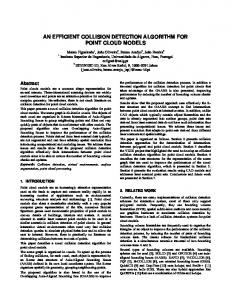
(a) Pipeline for collision or distance computation: The sensor data is first represented as a collision map constructed in T0 time. Next, the collision map is first converted into a set of boxes in T1,1 time. Finally, a broad-phase data structure is constructed in T1,2 time in order to manage these boxes. The overhead to prepare the sensor data is T1 = T1,1 + T1,2 . Once the data is prepared, the actual time to perform N collision or distance queries is T2 = N · Tq , where Tq is the time cost for a single query. In traditional approaches, N is assumed to be infinite, while for sensor data, N is usually small (< 1,000).

sensor data

octree

collision check distance comp.

(b) By supporting the collision or distance query directly with the sensor data represented as an octree, we no longer need the long conversion pipeline from octree to broad-phase structures and thus can completely avoid the main overhead T1 . Fig. 1: Comparison between possible pipelines for environment representation and collision detection.

construction step can be expensive. For sensor data, n is the number of boxes computed from sensor data and can be as high as 10,000. A. Amortized broad-phase Algorithm Our first method attempts to reduce the construction time of a dynamic AABB tree, i.e., T1,2 in Equation 2. Instead of constructing a high-quality dynamic AABB tree, we start with a low-quality binary tree and then gradually improve it during the following actual queries. The initial binary tree is constructed by using the well known space-filling Morton curve [18] – also known as the Lebesgue and z-order curve – to order all the boxes converted from the sensor data. We assume that the enclosing AABB of the entire environment is known. We take the barycenter of each of the n boxes as its representative point. By constructing a 2k · 2k · 2k lattice within the enclosing AABB, we can quantize each of the three coordinates of the representative points into k-bit integers. The 3k-bit Morton code for a point is computed by interleaving the successive bits of its quantized coordinates. Figure 2 shows a 2D-example of this construction. Sorting the representative points in increasing order of their Morton codes will lay them out in order along the Morton curve. Therefore, it will also order the corresponding boxes in a spatially coherent way, which directly determines a binary tree structure for the set of boxes. The time cost of this new tree construction method is dominated by the time to sort n 3k-bit integers, which is of time complexity O(3k · n) if we use radix sorting. The AABB tree constructed as above may not be as effective at culling as the high-quality AABB tree constructed with traditional approaches and therefore the timing cost of each actual query can increase, i.e., Tq item in Equation 2 can be larger. To overcome this problem, our solution is to incrementally refine the initial binary tree while performing each query. First, we encode each traversing path connecting the tree root node to one of the leave nodes as an O(log n)-bit integer, according to whether the left or right child is selected

during the traverse. Next, while performing the actual query, we periodically select one of the traversing paths and recompute the bounding boxes for all the nodes on the path. We begin from the leaf node, which has time complexity O(log n). Then after (at most) n iterations, the binary tree will become an AABB tree that is able to cull effectively. In practice, we have observed that the dynamic tree’s culling efficiency can be almost as good as the near-optimal binary tree in only a few iterations. As a result, we can assume that the actual query cost when using the amortized method is Teq = Tq + O(log n).

Fig. 2: Example 2-D Morton curve. According to the first two bits of the Morton code, we can order the objects in a hierarchical manner.

B. Proximity Computation using Octrees The amortized method cannot avoid the overhead of T1,1 in Equation 2, which can still be expensive for large sensor data. To avoid such overhead, our second method performs proximity queries directly on the sensor data in the form of an octree (as shown in Figure 1(b)); this completely avoids the long pipeline shown in (Figure 1(a)) required to prepare sensor data. In other words, we use the octree as a lowquality broad-phase structure for the sensor data. Octrees may not be as efficient at culling as a dynamic AABB tree, so the cost for a single collision or query cost can be larger than using the traditional pipeline, i.e., Teq0 > Teq > Tq . However, as

Algorithm 1: collisionRecurse(node1 , node2 ) 1 begin 2 if node1 .isLeaf() and node2 .isLeaf() then 3 if overlap(node1 .bv, node2 .bv) then 4 narrow-phase collision between the octree box in node1 and the object in node2 return collision status

5 6 7 8 9

10 11 12

if node2 .isLeaf() or (node1 .hasChildren() and node1 .bv > node2 .bv) then for i = 1 to 8 do if node1 .child(i).occupancy prob() > threshold then collisionRecurse(node1 .child(i), node2 ) else collisionRecurse(node1 , node2 .leftChild()) collisionRecurse(node1 , node2 .rightChild())

only a small number of queries are performed for one frame of sensor data, the saving on sensor data preparation time may make this strategy more efficient than the amortized strategy. We will now illustrate the use of this algorithm to perform collision checking between an articulated robot and the sensor data. The desired query can be implemented as a collision query between trees: the sensor data is represented as an octree and the robot is represented as a binary dynamic AABB tree. The algorithm is shown in Algorithm 1, which is a recursive method. We start with two root nodes of the two trees. If both of them are leave nodes, we perform the narrow-phase collision between the object corresponding to the given dynamic AABB tree node and one cubic cell in the octree. Otherwise, we need to check for collisions between the subtrees rooted at the corresponding two nodes. If the given octree node is not a leaf node, we recursively perform collision queries between the given dynamic AABB node and each of its eight children nodes. Otherwise, we recursively perform collision queries between the given octree node and the two children of the given dynamic AABB node. The recursion continues until the collision is detected. One major issue is mentioned in Algorithm 1 at line 8: we only perform collision queries for octree cells with occupancy probabilities larger than a given threshold. This is because the octree representation of the sensor data can encode uncertain or unknown regions in the environment, and we want the result computed by the new method to be consistent with the result provided by the simpler pipeline in Figure 1(a), where octree cells are converted into boxes only if their occupancy probability is larger than a given threshold. Similar recursive traversal can be used to handle the distance query between the robot and sensor data. Moreover, a binary tree can also be used to represent other types of data; e.g., a mesh can be represented as a binary AABB or OBB tree [9] and a geometric primitive (e.g., a sphere) can be represented as a binary tree with only the root node. As a result, the same recursive formulation can be used to handle the proximity query between the sensor data and either a

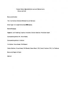
mesh or a geometric primitive. C. Collision Checking with Uncertain/Unknown Regions The data gathered by various sensors tend to have error and noise. Many sensors only have limited precision, which results in sampling error in the sensor data. Often, part of the environment may not be observed by the sensor, because sensors only have limited field of view and may have a large blind spot. Moreover, the camera or laser may not be perfectly calibrated; thus the generated point clouds may have systematic bias. It is important to handle the uncertain or unknown part of the sensor data so that robots can work robustly in real world scenarios. The unknown or uncertain regions are usually assumed to be collision-free, e.g., such an optimistic assumption is made in [13]. This assumption can cause serious problems in some cases. In the example shown in Figure 3(a), the sensor mounted on the robot’s head cannot cover the region near the robot’s left arm. Therefore, given a path for the left arm moving through the unknown region, the collision checking routine will always assume it to be collision-free, even if obstacles exist in that region. Our solution here is to compute a set of boxes representing different regions in the unknown space that intersect with the swept volume of the robot’s path. Only boxes with the largest occupancy probability are returned, because they are the most important regions to check when determining whether the given path is collision free. Given these boxes as shown in Figure 3(b), users can implement different strategies according to different applications. For example, the robot can try to avoid the unknown regions completely, minimize its motion through the unknown regions or actively sense the unknown regions to gain more information about them. The intersection between the unknown space and the swept volume of the robot’s path can be performed by checking the collisions between the octree and a series of samples on the path. Each collision query can be performed based on a recursive method similar to Algorithm 1. V. R ESULTS In this section, we present the performance of our new collision checking and distance computation algorithms when handling the sensor data. In the first experiment, we use a synthetic environment. First, we generate 300 randomly located objects (100 spheres, 100 boxes and 100 cylinders). We then construct a dynamic AABB tree broad-phase structure to manage these objects. Next, we randomly generate an octree structure with 7, 784 cells to simulate the sensor data. Our task is to perform collision or distance queries between the dynamic AABB tree and the sensor data. The reported performance for a single query is the average of the cost for 1, 000 queries. For all experiments on collision query, we compare the overall timing when performing 10 and 100 queries. For all experiments on distance query, we only compare the overall timing when performing a single query, because distance query is much more expensive than collision query.

(a) Collision checking only performed between the planned trajectory and the regions that are known to be occupied (the blue part) in the sensor data.

(b) Collision checking is performed between the planned trajectory and both the regions that are known to be occupied (the blue part) and the unknown regions in the sensor data.

Fig. 3: The environment representation can contain unknown or uncertain regions in the environment. In the case shown by (a), the sensor on the robot’s head cannot cover the region near its left arm. Therefore, a path for the left arm will always appear valid if we ignore unknown regions of the environment and make an optimistic assumption, even though obstacles could possibly exist in that region. Our solution is shown in (b), where we compute a set of boxes (shown in brown) that cover the intersections of robot links and unknown parts of the environment. Using these boxes, a notion of cost can be easily defined by the user, e.g., using the sum of the occupancy probability of all the boxes.

First we compare the performance between our amortized approach and the traditional non-amortized method and the results are shown in Table I. We can see that the amortized approach saves more than 50% of the broad-phase structure construction time, while the actual collision query is only slightly slower. According to this result, the amortized approach is faster than traditional methods when the number of actual queries is 10 and 100. As a matter of fact, the amortized approach is faster than traditional methods if the number of actual queries is smaller than 38, 300, which is much larger than the number of collision queries that can be performed during one sensor data frame. Next, we compare the performance between the baseline pipeline in [13] and our new pipeline. The results for the collision query are shown in Table II. In Table II(a), all the objects are represented as primitive shapes; and the octree is also converted into primitive boxes for the baseline pipeline. In Table II(b), the objects and boxes generated from octree are in the form of meshes. In the first case, the actual collision cost in the new pipeline is about two times the cost in the baseline pipeline, but the saved overhead cost is much larger than the actual query cost of a single query. As a result, the new pipeline performs better than the baseline pipeline if the actual number of queries is smaller than 300. In the second case, even the cost of a single query in the new pipeline is smaller than the baseline pipeline. The results for the distance query are shown in Table III. As in the collision case, the overhead cost is saved in distance query, and the overall performance is improved in the new pipeline. However, as the distance query is much more expensive than the collision query, the performance improvement caused by saving the overhead of data preparation is not as large as in the collision case. Moreover, note that we assume that all the steps in both pipelines can share the data efficiently, and therefore we can ignore the data transmission overhead between different steps. For distributed robot systems, such transmission overhead can be large and therefore we under-

estimate the performance improvement caused by the new pipeline, because the new pipeline has fewer steps than the baseline pipeline. In the second experiment, we perform collision or distance queries between a PR2 robot and the sensor data. The PR2 robot has 88 links, some in the form of primitive geometric shapes (e.g., cylinders and spheres) and others represented as meshes. The sensor data is an octree with 24, 803 cells. For collision queries, the PR2’s average penetration depth into the obstacles is 2.8 cm. For distance queries, the PR2’s average distance to the obstacles is 3.4 cm. Note that collision or distance queries are slow in case of small penetration depth or small distance to the obstacles, since the AABB cannot perform culling effectively in such cases. As a result, the scene is challenging for both collision and distance queries. The results are shown in Table IV; we observe similar performance improvements on real-world sensor data with the PR2 robot, as in the synthetic case. From these results, we can see the difference between the baseline pipeline using the amortized approach and the new pipeline. The amortized approach only reduces the overhead instead of completely avoiding it, but the performance reduction on a single actual query is small. The new pipeline completely avoids the overhead, but the time cost for one actual query may be notably larger than the traditional pipeline. As a result, the amortized approach is more suitable for cases where the number of actual queries per sensor frame is large, e.g., when the environment does not change frequently and the sensor frame rate is small; or when there are only a few obstacles in the environment. The method using the new pipeline is more suitable for dynamic environments with high sensor data frame rates, or for environments with many obstacles. Moreover, we have observed that the collision query benefits more from our new pipeline than the distance query, since the distance query is usually more expensive and the initialization overhead is less significant. Finally, the speedup caused by the new pipeline is more considerable for scenarios with many obstacles, since the initialization overhead increases with the number of obstacles. non-amortized amortized

T1 2.07 0.92

Tq 4.49 · 10−3 4.52 · 10−3

T1 + 10 · Tq 2.11 0.96

T1 + 102 · Tq 2.52 1.37

TABLE I: Performance comparison between baseline pipeline with and without amortized broad-phase structure construction (in ms). The highquality broad-phase structure computed by non-amortized algorithm improves the total computation only when there are more than Nmin = 38333 collision queries for one frame of sensor data, and the total time required for Nmin queries is 174 ms, which is much longer than sensor data’s update period (30 ms for data arriving at 30 Hz).

VI. C ONCLUSIONS We have presented two approaches for efficiently performing collision and distance queries on sensor data. The first method amortizes the sensor data pre-processing overhead over all the queries, and is suitable for static or simple environments. The second method shortens the traditional

baseline pipeline our pipeline

T1,1 2.283 0

T1,2 5.389 0

Tq 0.022 0.048

T1 + 10 · Tq 7.89 0.48

T1 + 102 · Tq 9.872 4.8

(a) Objects and boxes are in the form of geometric primitives

baseline pipeline our pipeline

T1,1 2.697 0

T1,2 5.465 0

Tq 0.317 0.075

T1 + 10 · Tq 11.3 0.75

T1 + 102 · Tq 39.9 7.5

baseline pipeline our pipeline

T1 0.131 0

Tq 0.00127 0.00131

T1 + 10 · Tq 0.1437 0.0131

T1 + 102 · Tq 0.258 0.131

(a) PR2 collision

baseline pipeline our pipeline

T1 0.163 0

Tq 0.039 0.048

T1 + Tq 0.202 0.048

(b) Objects and boxes are in the form of meshes

(b) PR2 distance

TABLE II: Collision query performance comparison between the baseline pipeline in [13] and our new pipeline (in ms). In both pipelines, the 300 objects in the environment are in the form of primitive geometric shapes or meshes. For the baseline pipeline, the boxes generated from the octree are also represented as primitive boxes or meshes, respectively. When objects are in the form of primitive geometric shapes, the broad-phase structure computed by the baseline algorithm improves the total computation only when there are more than Nmin = 2959 collision queries for one frame of sensor data, and the total time required for Nmin queries is 72.77 ms, which is much longer than sensor data’s update period (30 ms for data arriving at 30 Hz). When objects are in the form of meshes, the average query time given by our new pipeline may even be faster the the average query time provided by the baseline pipeline.

TABLE IV: Collision and distance query performance comparison between the baseline pipeline in [13] and our new pipeline on the PR2 robot (in ms). For collision query, the broad-phase structure computed by the baseline algorithm improves the total computation only when there are more than Nmin = 3275 collision queries for one frame of sensor data, and the total time required for Nmin queries is 4.29 ms. For distance query, the broad-phase structure computed by the baseline algorithm improves the total computation only when there are more than Nmin = 18 collision queries for one frame of sensor data, and the total time required for Nmin queries is 0.87 ms.

baseline pipeline our pipeline

T1,1 2.665 0

T1,2 5.381 0

Tq 23.98 17.40

T1 + Tq 32.03 17.40

(a) Objects and boxes are in the form of geometric primitives

baseline pipeline our pipeline

T1,1 2.871 0

T1,2 5.413 0

Tq 68.03 61.86

T1 + Tq 76.31 61.86

(b) Objects and boxes are in the form of meshes TABLE III: Distance query performance comparison between the baseline pipeline in [13] and our new pipeline (in ms). In both pipelines, the 300 objects in the environment are in the form of primitive geometric shapes or meshes. For the baseline pipeline, the boxes generated from the octree are also represented as primitive boxes or meshes, respectively. In this experiment, our new pipeline not only avoids the initialization overhead and also behaves better than the baseline pipeline on average distance query time. This is due to the fact that the octree structure may perform distance culling more efficiently than the hierarchy tree structure.

pipeline by directly performing queries between the robot links and an octree that represents sensor data. This approach completely avoids the data pre-processing overhead, and is suitable for dynamic or complex environments. We demonstrated the performance of the two methods on synthetic benchmarks and on environments constructed using the RGB-D sensor mounted on the PR2 robot. Our new approach also supports collision queries for sensor data with uncertain or unknown regions. In summary, the techniques we propose in this paper will make collision checking and distance queries with real sensor data more efficient; will improve the reactive behavior of robots operating in unstructured environments; and will allow them to deal better with uncertain information about the environment. For future work, we are interested in further improving the collision checking and distance query implementations. We are also interested in applications of this work to motion planning and active sensing, e.g., we would like to design strategies for gaining more information about uncertain or unknown parts of the environment. R EFERENCES [1] E. Coumans, “Bullet,” http://bulletphysics.org/.

[2] “Open dynamics engine,” http://www.ode.org. [3] T. C. Hudson, M. C. Lin, J. Cohen, S. Gottschalk, and D. Manocha, “V-COLLIDE: accelerated collision detection for VRML,” in Proceedings of Symposium on VRML, 1997, pp. 117–124. [4] S. Gottschalk, M. C. Lin, and D. Manocha, “OBBTree: a hierarchical structure for rapid interference detection,” in Proceedings of SIGGRAPH, 1996, pp. 171–180. [5] “Box2d,” http://box2d.org. [6] R. B. Rusu, N. Blodow, Z. C. Marton, and M. Beetz, “Close-range scene segmentation and reconstruction of 3d point cloud maps for mobile manipulation in domestic environments,” in Proceedings of International Conference on Intelligent Robots and Systems, 2009, pp. 1–9. [7] M. Muja, R. B. Rusu, G. Bradski, and D. G. Lowe, “REIN - a fast, robust, scalable recognition infrastructure,” in Proceedings of International Conference on Robotics and Automation, 2011, pp. 2939–2946. [8] K. M. Wurm, A. Hornung, M. Bennewitz, C. Stachniss, and W. Burgard, “OctoMap: A probabilistic, flexible, and compact 3D map representation for robotic systems,” in Proceedings of the ICRA 2010 Workshop on Best Practice in 3D Perception and Modeling for Mobile Manipulation, 2010. [9] J. Pan, S. Chitta, and D. Manocha, “FCL: A general purpose library for collision and proximity queries,” in Proceedings of International Conference on Robotics and Automation, 2012, pp. 3859–3866. [Online]. Available: http://gamma.cs.unc.edu/FCL [10] C. Ericson, Real-Time Collision Detection. Morgan Kaufmann, 2004. [11] D. J. Tracy, S. R. Buss, and B. M. Woods, “Efficient large-scale sweep and prune methods with aabb insertion and removal,” in Proceedings of the IEEE Virtual Reality Conference, 2009, pp. 191–198. [12] S. Bandi and D. Thalmann, “An adaptive spatial subdivision of the object space for fast collision detection of animating rigid bodies,” Computer Graphics Forum, vol. 14, pp. 259–270, 1993. [13] R. B. Rusu, I. A. S¸ucan, B. Gerkey, S. Chitta, M. Beetz, and L. E. Kavraki, “Real-time perception guided motion planning for a personal robot,” in In Proceedings of International Conference on Intelligent Robots and Systems, 2009, pp. 4245–4252. [14] A. Leeper, S. Chan, and K. Salisbury, “Point clouds can be represented as implicit surfaces for constraint-based haptic rendering,” in Proceedings of International Conference on Robotics and Automation, 2012, pp. 5000–5005. [15] J. Pan, S. Chitta, and D. Manocha, “Probabilistic collision detection between noisy point clouds using robust classification,” in Proceedings of International Symposium on Robotics Research, 2011. [16] B. Alexe, T. Deselaers, and V. Ferrari, “What is an object?” in Proceedings of International Conference on Computer Vision and Pattern Recognition, 2010, pp. 73–80. [17] I. A. S¸ucan, M. Kalakrishnan, and S. Chitta, “Combining planning techniques for manipulation using realtime perception,” in Proceedings of International Conference on Robotics and Automation, 2010, pp. 2895–2901. [18] G. Morton, “A computer oriented geodetic data base and a new technique in file sequencing,” IBM Ltd, Ottawa, Canada, Tech. Rep., 1966.