Real-Time Multiple Event Detection and Classification

Real-Time Multiple Event Detection and Classification in Power System using Signal Energy Transformations Ravi Yadav, Ashok Kumar Pradhan, Senior Member, IEEE, and Innocent Kamwa, Fellow, IEEE

Abstract—Real-time multiple event analysis is important for reliable situational awareness and secure operation of power system. Multiple sequential events can induce complex superimposed pattern in the data and are challenging to analyze in real-time. This paper proposes a method for accurate detection, temporal localization, and classification of multiple events in real-time using synchrophasor data. For detection and temporal localization, a Teager-Kaiser energy operator (TKEO) based method is proposed. For event classification, a time series classification based method using energy similarity measure (ESM) is proposed. The proposed method is tested for simulated multiple event cases in IEEE-118 bus system using DigSilent/PowerFactory and real PMU data for India grid. Index Terms—Multiple events, event detection, event classification, temporal localization, Teager-Kaiser energy operator, energy similarity measure.

I. I NTRODUCTION

M

ONITORING and analysis of power system disturbances are important to pinpoint the causes of abnormal system operation, for evaluating protection and control schemes, and ensuring fast system restoration [1]. During disturbance, inadequate understanding of system dynamics and improper control action can escalate the stressed situation [2]. Disturbance monitoring is important from view point of fast control actions during emergency state to safeguard the system security. Phasor measurement units (PMUs) with time synchronized voltage and current phasor data in a wide area measurement system (WAMS) enhances power system visibility [3]. In existing practice PMU data after a disturbance are stored in a separate disturbance file for postmortem analysis [4]. Meanwhile advancement in synchrophasor technology and fast data delivery makes analysis of disturbances in real-time feasible. There are two main approaches used for real-time event analysis: model-based and data-based. Databased techniques are independent of system operational and structural changes in contrast to model-based, therefore are advantageous [5]. Most of the previous work on real-time event analysis focuses on analyzing single isolated events in power system using synchrophasor data [5]- [6]. In which different disturbance indicators like voltage [5], frequency [6], [7], voltage angle [8]. For event detection signal features like change in frequency (∆f ), change in voltage (∆V ), and rate of change of frequency (df /dt) are used [3], [5], [9], which can suffer from poor time resolution and have limitation in segregating events from oscillations. Therefore, an alternate detection method is proposed in the paper using Teager-Kaiser energy operator [10]. It only uses two sample past data for calculation, thereby

offers low computational burden and high time resolution. For power system applications, it is applied for determining damping factor and frequency of different frequency modes in power system oscillations [11] and for fault identification in induction motor [12]. In previous applications TKEO is applied on amplitude or frequency modulated signals to obtain the energy signature of a signal [13] along time but not yet applied on synchrophasor data for multiple event detection problem. For classification of events several feature based methods are proposed in the available work, where frequency or timefrequency domain methods like discrete wavelet transform (DWT) [2], discrete Stockwell-transform [7] etc. are used. On the basis that different classes of events introduce distinct frequency modes in the PMU signals, which can be utilized for classification. However, this is only true in case of single events. For multiple events individual frequency modes by each sequential event superimposes making classification challenging [14]. Also, there can be numerous combinations of events of different classes, locations, or magnitudes that further complicate the multiple event analysis [15]. Thus, classification based on temporal patterns in the data can be an alternative approach. Time series classification methods use temporal sequence in a query signal (i.e. test sequence (TS)) to quantify its similarity with training sequence (TrS) for classification [16]. Typical time series classification approaches are instance based (using euclidean distance or dynamic time warping (DTW)), shapelet based [17], feature based [16] etc. Shapelet based methods have limitation in searching for shapelets in a large database. Feature based methods rely heavily on strong classifiers to achieve high accuracy [16]. An instance based approach is proposed in the paper using 1NN classifier with energy based similarity measure (ESM). It uses cross Teager-Kaiser energy operator (CTKEO) to determine similarity between time series in terms of cross-energy of query signals [18]. Unlike Euclidean distance and correlation coefficients, ESM includes temporal information and relative change of two time series, therefore is advantageous. It is used in [19] for gene data clustering. 1NN classifier model along with different similarity measure is extensively used in TSC problems because of simplicity and time efficiency [16], therefore preferred in the method. A limited work is available on real-time multiple event analysis, propositions like [20] and [21] considered detection and classification of multiple line trip events only. But ignored

Frequency (Hz)

Frequency (Hz)

50 49.99 49.98 49.97 0.6

0.8

1

1.2

1.4

1.6

1.8

50

49.9 8

10

12

49.9

49.8 3.5

4

Time (s)

16

18

20

22

(b) Frequency (Hz)

Frequency (Hz)

(a)

3

14

Time (s)

49.85 4.5

5

A. Multiple Event Detection and Temporal Localization Detection of multiple events is challenging using conventional detection parameters like ∆f, ∆V or (df /dt). For example the frequency plot and (df /dt) response for a multiple event case is shown in the Fig. 2 (a) and (b). Effect of superimposed responses and oscillation are evident in (df /dt) signal which compromise its detection capabilities. Therefore, a TKEO based detection method is proposed in this work. TKEO is a non-linear energy operator that determines instantaneous energy of a univariate signal. It shows high sensitivity to transient changes in a signal and low alterations during oscillations and static variations. TKEO is represented in the discrete domain as: ψd [x(n)] = [x(n)]2 − x(n − 1)x(n + 1)

(1)

where x(n) is a discrete signal and ψd [x(n)] is its instantaneous signal energy at nth sample. ×10-3

df/dt (Hz/s)

50.02 50 49.98 49.96

1

2

3

4

5

6

7

2 0 -2 -4

Time (s)

1

2

3

4

Time (s)

5

6

7

(a) (b) Fig. 2. Plot of (a) Frequency (b) (df /dt) signals for a multiple event example (LL event at 1s, GL event at 2.2s and LT event at 4s).

|ψd(∆f)|

6

×10-4

×10-4 4 2 0 0.98 1

4 2 0

Trans

ψd

1

2

3

Time (s)

-7

10 0

×10

1.02

1.2

Osc

1.4

ψd (∆f)

(∆f)

4

5

Fig. 3. Plot of ψd signal for the multiple event example.

49.95

Time (s)

49.95

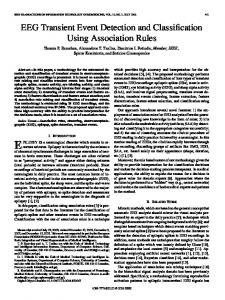
II. P ROPOSED M ETHOD A data-based approach is proposed in the work for realtime multiple event analysis. Frequency signals are used as disturbance indicator in the work. As frequency varies globally through out the system during an event in comparison to local variables like voltage and voltage angles. Which enables lower processing data size and consequently fast computation. Majority power system events in the India grid are categorized into four main types: fault (FLT), generation loss (GL), load loss (LL), and line trip (LT) (excluding LT due to the fault events) [24]. These events influence rotor angle and voltage stability of a power system. Therefore their analysis in realtime is necessary to enable fast system control during emergency. Real PMU data from Indian grid for each class of event is shown in Fig. 1.

Frequency (Hz)

other commonly occurring events like generation loss, load loss, etc. A method based on principal component analysis (PCA) for real-time multiple event analyses is proposed in [22] that can only detect and classify multiple events causing net loss in generation or load power, which does not happen in all cases. In [14], a method based on sparse unmixing is proposed overlooking the complexities observed for a large power system. A cluster based sparse coding technique is proposed in [15] for a large power system. It uses different combination of time shifted training patterns to calculate sparse coefficients with the test sequence to detect and classify multiple events. In this work, a method for detection, temporal localization, and classification of multiple events is proposed using signal energy transformation. For event detection and temporal localization, TKEO is applied to frequency signal from synchrophasors to detect signal energy changes during disturbance. TKEO has ability to segregate events from oscillations, which is advantageous in detecting events like line trip. TKEO uses only 2 sample past data that improves the time localization compared to other detection variables like (df /dt). Variation in signal’s energy at event inception is an indicator of closeness of a PMU to a disturbance. Therefore, can help in obtaining physical location of an event in a network i.e. network localization of event. For multiple event classification, an instance based TSC method is proposed using ESM similarity measure. ESM uses 2 sample backward difference for calculation tracing both temporal attributes and relative variation of two time series. It follows superposition property enabling similarity evaluation among superimposed events. For classification ESM uses only 10 sample (100 ms for 100Hz sampling rate) disturbance data offering near real-time classification. Available methods [14], [22], use large temporal sequences of 5-10 s for detection and classification of events. On the other hand proposed method requires only 100 ms of the data providing the advantage of low processing burden and fast computation. Further, TKEO provides an advantage of faster time localization compared to the available methods. In addition to multiple event analysis the proposed method also considers network localization of event. The method is not affected by pre-disturbance operating state, topology of a system and class combination of sequential events. Examples, training, and test cases are simulated for IEEE-118 bus system [23] using DigSilent/PowerFactory. Proposed method is also validated for real PMU data for Indian grid.

50.05 50.04 50.03 50.02 0.6

0.8

1

1.2

1.4

Time (s)

(c) (d) Fig. 1. Real PMU data for Indian grid for (a) FLT, (b) GL, (c) LT, and (d) LL events.

When applied to a ∆f (fmeas − fbase ) (where fmeas is the measured frequency and fbase is the base frequency 50Hz) TKEO produces impulsive change in the signal energy at event inception and negligible variations during oscillation. During the transients ψd can be approximated as: ψdT rans [∆f (k)] ≈ [∆f (k)]2 (2) T rans where ψd [∆f (k)] is the energy value during transient at k th instant. The oscillations in PMU frequency signals due to a disturbance can be approximated as damped sinusoid (∆f (n) =

A(n)sin(φx (n)) [11], where φx (n) = ωx (n).n + θx . The TKEO response for damped oscillation is: 2

≈ A(n) .ω(n)

PMU 15 PMU 11

(3)

where ψdOsc [∆f (n)] is the signal energy during oscillation at nth instant, A(n) is the amplitude, and ω(n) is the frequency of damped oscillation [11]. The oscillation in frequency signal is sufficiently damped in a power system and amplitude reduces below ±0.01Hz within 2-5 fundamental cycles. On the other hand, ω(n) lies in a range of 0 − 2Hz (including both inter-area and intra-area oscillations) [11]. Therefore, during transients (A(n).ω(n))2 1Hz, (ii)   df > 0.124Hz/s (iii) 85% nominal voltage for more dt than 5s [9]. More  stringent  detection criteria ∆V ± 10%, df ∆f ± 0.05Hz, and ± 0.05Hz/s are recommended in dt [5]. Using same criteria ∆f ± 0.05Hz detection threshold is calculated in present application. To indicate detection of an event an index D is defined that compares | ψd | with a threshold γ. The conditional statement for D is: ( T ran 1 if | ψdi |≥ γ (4) D= 0 else T ran where | ψdi | is the absolute transient energy value for th i PMU (taking absolute eliminates the negative jump in ψd during transients which helps in setting a single positive threshold), i ∈ (1, 2, 3....n), n are the total number of buses. For temporal localization, detection time td is saved. 1) Network Localization of Events: For determining physical location of an event in a network, conventionally ∆f and df /dt signals are used [3]. But as mentioned earlier these parameters perform poorly in case of multiple events. However, peak value of signal energy (ψd ) is capable of indicating relative closeness of a PMU from an event. Because in (2) it is shown that ψd at transient depends on ∆f magnitude which will be distinct depending upon the electrical distance of a PMU from a disturbance. Also, since ψd unlike ∆f or df /dt is not affected by oscillation, it provides a better alternative for network localization of events. For example, consider an LT event on line 11-13 of the system shown in Fig. 4 (a) with PMUs at buses 11, 2, 1, and 15. The highest ψd value is obtained for PMU at bus-11 (Fig. 4. (c)), which happens to be electrically closer to the disturbance than other PMUs. Thus, TKEO has potential of providing network localization of events accurately.

B. Classification of Multiple Events The classification method first acquires a query test sequence from streaming PMU frequency data by assigning a classification data window of size N. Thereafter, individual training sequences (TrS) of different classes are sequentially compared with the TS to obtain ESM values. The class of TrS attaining highest ESM value is assigned to the event by the

(a) PMU-11 PMU-2 PMU1 PMU-15

50.02 50.01 50 1

1.1

1.2

1.3

1.4

1.5

1.6

×10-4

|ψd (∆f)|

2

Frequency (Hz)

ψdOsc [∆f (n)]

PMU 2

PMU 1

ψd (PMU11) ψd (PMU15)

2

0 0.99

ψd (PMU2) ψd (PMU1)

1

1.01

1.02

Time (s)

Time (s)

(b)

(c)

Fig. 4. (a) Section of IEEE-118 bus system with PMU positions and Plot of (b) Frequency signals (c) ψd for a LT event at line 11-13.

1NN classifier. This process is repeated for all other sequential events. The classification methodology is shown in Fig. 5. k

z C1

z TrS of C Class

z Cn

z TrS of Cn Class

Fig. 5. Classification methodology.

Acquiring TS can be challenging in a large power system. Since the size of processing data could be large because of substantial PMU measurements. Therefore, to keep the size of data low, a single PMU showing maximum deviation in energy ψd (MDE) (i.e. PMU in close proximity to the disturbance) is used for TS. This serves two purposes (i) the dimensionality of TS is reduced to just N × 1 and (ii) dominant pattern is used for classification. 1) Energy Similarity Measure: ESM quantifies the similarity between the two time series in terms of energy of interaction or cross-energy. It is obtained by normalizing crossenergy between two time series [18] and is expressed as: √ PN 2 n=0 Ω(x(n), y(n)) ESM (x, y) = PN p Ω(x(n), x(n))2 + Ω(y(n), y(n))2 n=0 (5) where N is the length of the classification window, Ω(x, y) is the cross-energy measure between x and y time series. Cross-energy measure is calculated using cross Teager-Kaiser energy operator (CTKEO) [25] expressed in discretized form using two sample backward difference as: Ω(x(n), y(n)) = x(n − 1)y(n − 1)− 1 (x(n)y(n − 2) + y(n)x(n − 2)) (6) 2 To understand the cross-energy measure, consider two sinusoids: x(t) = Acos(φx t) and y(t) = Bcos(φy t), where φx = ωx t + θx and φy = ωy t + θy . On applying CTKEO the cross-energy value between the signals can be approximated as : Ω(x, y) = A.B[(ωx + ωy )2 cos((ωx − ωy )t)+ (ωx − ωy )2 cos((ωx + ωy )t)] [25]

(7)

(8)

when signals have different frequencies (ωy = ωx + ∆ω) their cross-energy becomes: Ω(x, y) = A.B(2ωx + ∆ω)2 cos((∆ω)t)

(9)

From (8) and (9) it can be inferred that when two signals have same time symmetry their cross-energy value is static along the time shown in Fig. 6 (b), on the other hand distinct signals generate periodic variations in cross-energy as shown in Fig. 6 (d).

1 0.6 0.4 0.2 0

x(t) y(t)

0.5 0

0.037 6.6

6.7

6.8

6.9

7

6.6

6.7

Time (s)

0.04 0.02 0 -0.02 -0.04

0 -0.5 6.7

7

(b) x(t) y(t)

6.6

6.9

Ω (x,y)

x(t) & y(t)

(a)

6.5

6.8

Time (s)

0.5

6.8

6.9

7

7.1

6

Time (s)

6.5

7

Time (s)

(c)

(d)

Fig. 6. (a) Signal waveforms (where A and B is 0.8 and 0.5, signal frequencies are 50Hz ) (b) respective Ω(x, y) and (c) Signal waveforms (where signal amplitudes are same but frequencies are fx = 50Hz and fy = 60Hz ) (d) respective Ω(x, y).

On taking average of Ω(x, y) along a window of size N (where N should be (f s/(fx − fy ))) (where fs is the sampling frequency) the cross-energy comes closes to zero for distinct signals. This fact is used in ESM, where dissimilar signals produce ESM ≈ 0 and similar signals generate ESM closer to 1. On varying the window size, ESM remains unchanged for similar signals, but its peak overshoot increases in case of dissimilar signals. Nonetheless, reducing window size would slightly hamper the classification accuracy but drastically reduce the processing data size. A comparison between ESM response for sampling window size N and N/10 is shown in Fig 7, where other parameters of signals are same as in Fig. 6 (a). 1

ESM

0

2

4

MWD-GL

30

6

8

10

Time (s) Fig. 7. Plot of ESM for sample window size N and N/10

Few properties of ESM that are particularly favorable from multiple event classification point of view are: (1) Amplitude and time shift invariability: Two time signals with same symmetry but amplitude and time shifted yield same ESM values. This is Because the average of crossenergy values remain unchanged, therefore: ESM (x(n), (y(n − τ ) + a)) = ESM (x(n), y(n)) (10)

40

LL GL

0.5 0 0

10

20

30

40

Training sequences (TrS)

(b)

Fig. 8. Plot of MWD and (c) ESM (k+N) values for comparing P2 with TrS of GL and LL class.

Effectiveness of ESM in case of multiple events is compared with other widely used similarity measure, dynamic time warping (DTW) [26]. For a multiple event example in Fig. 2 (a) a test sequence for GL event is compared with training sequences (TrS) of GL and LL classes using DTW and ESM. For DTW, minimum warping distance for different training sequences are shown in Fig. 8 (a). It shows that the warping distances for GL and LL class training sequences are in close proximity, thereby challenging classifiers setting and accuracy. This is because of positive pre-disturbance shift in ∆f due to the previous LL event. That causes DTW to show more similarity for LL TrS ( produces +ve ∆f ) than GL TrS. ESM (k+N) (ESM at (k + N )th instant, where k is event inception time and N is length of classification window) values for two classes are sufficiently segregated as shown in Fig. 8 (b) ensuring easy settings and efficient classification. This is also confirmed for other multiple event cases, thereby confirming that ESM is a better perspective for multiple event classification. In the present work, a 1NN classifier model is used for time series classification with ESM as similarity measure. The classifier searches for the most similar TrS in the pattern space and classifies each event. The distance function of 1NN classifier in the method is considered as: d(Yi , Xj ) = max((ESMk+N (Yi∈m , Xj∈z ))) th

N N/10

0.5

-0.5 0

20

(a)

0.038

-0.5

MWD-LL

10

Training Sequences (TrS)

Ω(x,y)

x(t) & y(t)

-0.2

0.04

ESM(k+N)

Ω(x, x) = (A.B)(4(ωx )2 )

(2) Superposition property: This property of ESM is most principal to multiple event classification. As, the sequential events occur with a certain time gap the superimposition effect of one class of event will be lower on the other class. That would produce distinct cross-energy values for each superimposed event making their classification possible. ESM ((x1 + x2 ), y) = ESM (x1 , y) + ESM (x2 , y) (11) where, x1 and x2 are individual components of a overlapped time series. MWD

If two signals have distinct amplitudes, but same frequency i.e. (ωx = ωy ) then the cross-energy is:

th

(12)

where Yi is a TS for i event and Xj is the j TrS, ESMk+N is the distance measure. m are the number of events and z number of TrS in training database. Each step in detection and classification of multiple events is provided in the flow diagram of Fig. 9. The method first compares |ψd | values with a threshold γ, to ensure detection. Then ith PMU with MDE is indexed that provides T Sim for mth event. The indexed PMU also provides network localization of mth event. Than, T Sim is compared by 1NN with j th training sequence of class c (T rSjc )) using ESM(k+N) measure. Acquired class of the most similar TrS is assigned to mth event. C. Training Database Generation For training a large set of simulated single events are considered. A total of 2000 events in 118 bus system with

No

Segregate test sequence TS mi (n) indexed PMU. 1NN Classifier with ESM(k-N) measure

|Ψd |(n) > γ Yes Save td(n)

Network localization of mth event near PMU i.

Training Database c

Select TrS j

Assign the class label to mthevent.

Fig. 9. Flow diagram for the proposed method (online operation).

1500 FLT events (3φ,2φg,2φ,1φ at 20% and 80% of the line and for fault clearing time of 100ms and 500ms), 171 GL events (at all generator with 20%, 50%, and 80% loss of generated power), 186 LT events (at all lines) and 143 LL events (all loads with 20%, 50%, and 80% loss of load power) are considered. For all cases pre-disturbance frequency is maintained within a range of 49.97- 50.02 Hz as mandated by the Indian grid code [3]. For training, frequency signals from all buses are considered. That makes the size of initial training matrix as R × (2000 × 118) (where R is number of observations, which are taken as 1000 samples or 10s for training). For a large power system the training database needs processing to consider the effect of coherent groups and single line connections. Both the issues are discussed in detail and appropriate modifications are proposed. 1) Effect of Coherent groups (CGs): In a large power system there are multiple group of coherent buses with dissimilar frequency dynamics for an event. That can create confusion as to which response should be taken for training. It is preferable to include patterns from all coherent areas. According to [27], by taking an average of individual coherency matrices the effect of operating conditions can be eliminated and also the number of coherent groups k can be determined. Therefore, correlation (marker of coherency between frequency vectors of different buses for a set of 200 events are calculated and average of all correlation matrices is taken. Pearson coefficient of correlation is used for analysis (15).  1  E E [ρ(fi , fj )] 1 + · · · + [ρ(fi , fj )] Nc (13) [ρ(Fi , Fj )] = m where [ρ(Fi , Fj )] is the average correlation matrix, ρ(fi , fj )E is a correlation value for an event E between ith and j th buses and Nc number of events are considered. Image of the resultant correlation matrix is shown in Fig. 10 , where 3 groups are showing high correlation therefore k = 3.

Bus Index

1

20 40 60 80 100

0.9 0.8

20

40

60

80

100

Bus Index Fig. 10. Image of the average correlation matrix for 118 bus system.

Using these results, data for each event are clustered using k-Means technique by keeping k=3. Each cluster is replaced by its cluster mean because ESM value for it and other cluster

members remained in the margin of 0.9 < Avg(ESM ) > 1. Clustering reduces the training size to R × (2000 × 3). 2) Effect of single line connections (SLCs): Single line connections in a power system generate similar frequency responses for events of distinct classes like the equivalent representations shown in Fig. 11. For a radial connection (RC) in Fig. 11 (a), LL event (complete loss of load) and LT event (not due to a fault) will produce same active power imbalance in the grid. That in-turn would generate similar frequency responses at adjacent buses. Same is true for single line connection of generation in Fig 11 (b), for GL and LT event. This similarity in responses for different classes could confuse a classifier.

(a)

(b)

Fig. 11. Equivalent representation of (a) Radial connection (b) single line connection of generation in a power system.

Therefore, dissimilarity between responses of different classes in case of SLCs needs to be evaluated. For a RC (Line 12-117 and load 117) in 118 bus system the frequency patterns for LT and LL events are shown in Fig. 12 (a) and (b). The time symmetry of patterns are similar however there is a amplitude difference in frequency change (Because of extra damping offered by line resistance on the local area frequency in case of LL event). According to (8) cross-energy depends upon the product of magnitudes of two time series. Therefore, ESM will give distinct values for these two events in contrast to DTW that fails to distinguish two cases. The data for similar events in case of SLCs are first clustered using k-mean and than the cluster means are compared using ESM (detailed in section. II.C). Once showing least similarity are added as additional training sequences. Single line connections are system specific and need separate evaluation during training. 50.01

Frequency (Hz)

Calculate ψd (n) from Δf(n).

th

Index i PMU with max(ψd (n))

Frequency (Hz)

Streaming data at PDC from n PMUs.

P1 P2 P3

50.005

50 5

5.5

6

Time (s)

(a)

6.5

7

50.01

P1 P2 P3

50.005

50 5

5.5

6

6.5

7

Time (s)

(b)

Fig. 12. Patterns in ∆f for (a) LT event (L 12-117) and (b) LL event (Load 117) in 3 coherent areas.

3) Pruning: The size of a training matrix is substantially large (R × (1200 × 3)) for the present system. Therefore, TM should be efficiently pruned to ensure variability in TrS rather than repetition. For pruning, mean-shift clustering technique [28] is used. It is non-parametric and doesn’t need specifying number of clusters before hand. After clustering, the cluster means are saved in the training matrix. Pruning reduces the training size to just (R × (354)). III. R ESULTS To demonstrate the capability of the proposed method different test cases are simulated for IEEE-118 bus system shown in Fig. 13, using Digsilent/Powerfactory. There are two sets of cases considered for analysis: (i) unequal multiple events,

14 6

5

15

7

36 G

4 16

G

8

18

1 7

20

24

31 29

G

21

G

6 6

48

70

69 116

G

G

75

61

G 80

77

99 98

82

G

84

106 G

94 95

26

G

83

G

107

104 93

89 92

88

100 108

85 86

90

91

101

102

103

109

110 87 G

G

G SLCG-2

111 G

8

Frequency (Hz)

Frequency (Hz)

| ψd (∆f) |

γ

0

0

2

4

6

2

8

4

(d) 1

0.8 0.6

ESM (k+N)

GL LL LT FLT

0.4 0.2 2

3

4

6

Time (s)

Time (s)

5

6

7

8

GL LL LT FLT

0.8 0.6 0.4 0.2

9

2

3

4

5

6

7

8

Time (s)

(f)

Fig. 14. Plots of frequency signals for (a) case:A (b) case:B, ψd signals for (c) case:A (d) case:B, and ESM(k+N) for (e) case:A (f) case:B of a unequal multiple event cases.

G

96

7

0.02

(e)

97

23 115

γ

62

81 76

6

(b)

0.01

1

6 5

5

Time (s)

0.04

Time (s)

22 G 114

4

(a) 0.02

G

G

G

118

74

25 27

49

47

32 28

64

43

7 G 46 3 7 1 G

G

10 SLCG-1

30

113

63 5 1

45

G

9

G

58

50

35 19

3

112 G

Fig. 13. IEEE-118 bus system with highlighted SLCs.

According to (2), the event detection threshold (γ) for detection criteria of ∆f = ±0.05Hz comes as 0.0025, which is used for all test cases. As explained earlier the classification window size N should be (f s/(fx − fy ))). In a power system the inter-area and intra-area oscillation frequencies lie in the range of 0-2 Hz. Therefore, (fx − fy ) ≈ 2 and since f s = 100Hz the size N comes as 50 samples. But as established before that reducing N does not affect the ESM value for similar signals. Therefore, in the present method N/5 i.e. 10 samples window is used for classification. For the reduced window size the avg(ESM) for dissimilar signals remained below 0.3 that has no effect on classification. A. Cases of Unequal Multiple Event In several multiple event cases severe events tend to overshadow less severe sequential events making there detection and classification difficult. The proposed method is tested for two such cases: 1) Case:A: For this case four sequential events are considered a GL event at 1.2 s on generator 49 causing a loss of 160 MW generation, LT event at 2.5 s on line 100-103, LL event at 5.3 s on load 31 causing loss of 25 MW load, and a LL event ate 7.5 s on load 49 causing a loss of 87 MW load. The frequency plots at bus 19 and 100 are shown in Fig. 14 (a). On applying TKEO, the signal energy (ψd ) shows distinct peaks for all events with values more than the threshold as shown in Fig. 14 (c), thereby confirming detection of all events. Their detection times are 1.209 s, 2.518 s, 5.313 s, and 7.508 s. The ESM(k+N) values for first event are [GL = 0.85, LT = 0.35, LL = 0, F LT = 0.025]. For other events LT, LL, and LL classes have highest ESM values as shown in Fig. 14 (e). Therefore, 1NN assigns GL, LT, LL,

and LL classes to sequential events. That matches with the actual consideration. For network localization of events peak ψd values for different PMU signals are compared. The highest ψd value for four events are 0.012 (PMU-49), 0.004 (PMU-100), 0.01 (PMU-31), and 0.05 (PMU-49). Plot of ψd for different buses in case of first and third event is shown in Fig. 15 (a). Highest ψd value for each event is obtained for PMU closest to the disturbance location. Thus, the results for network localization of events are accurate as obtained by the method. 12

×10-3

×10-3 Bus-47 Bus-48 Bus-49 Bus-50

10 8 Event-01

6 1.255 1.26 1.265 1.27

Time (s)

8 6

5.32

Time (s)

0.04 0.03 0.02

Event-03

5.31

Bus-28 Bus-29 Bus-15 Bus-17

0.05 Bus2 Bus12 Bus-29 Bus-31

10

5.33

|ψd(∆f)|

G

2

(c) 56

6.55

49.5

8

59 57

6.5

50

55

54

44 34 38

6

Time (s)

PMU-15 PMU-6

50.01 50

50.01 50 5.4 5.6 5.8

50.5

|ψd(∆f)|

37

11

4

|ψd(∆f)|

33

13

12

3

53

52

117

2

ESM (k+N)

G

2

49.9 49.85

|ψd(∆f)|

1

42

41

Bus-49 Bus-100

G

G

G 40

RC-1

50 49.95

| ψd (∆ f)|

where magnitude and class of events are varied (ii) contiguous multiple events, where time gap and class combinations of events are changed. The reporting rate (RR) of PMU is considered as 100 frames per second (fps) according to IEEE standard [29]. The frequency measurements are taken from PMUs at all the buses. Although, with reduced PMUs the classification remains unaffected because the PMU chosen for TS (as mentioned in Section. II.B) always remain within the same coherent group. This is tested for optimal PMUs in the system using [30].

Bus-79 Bus-80 Bus-97 Bus-98

0.1

0.08 0.06 0.04

Event-02

5.41

5.42

Time (s)

5.43

Event-03

6.51

6.52

6.53

Time (s)

(a) (b) Fig. 15. Plots of ψd for adjacent buses for (a) event-01 and 03 for case:A (b) event-02 and 03 for case:B of a unequal multiple event cases.

2) Case:B: In this case three sequential events are considered, a FLT event (3φ FLT cleared in 50 ms) at 2 s on Line 6-7, a LT event at 5.4 s on line 15-17, and a LL event at 6.5 s on load 80 causing a loss of 130 MW load. The frequency plots at bus-15 and 6 are shown in Fig. 14 (b). Just like the previous case, ψd obtains distinct peaksfor each event as shown in Fig. 14 (d), confirming detection of all events. Their detection times are 2.008 s, 5.416 s, and 6.511 s. ESM(k+N) values for first event are [F LT = 0.78, GL = 0, LL = 0.02, LT = 0.39]. For other events LT and LL classes are showing highest ESM values (Fig. 14 (f)) which means output of 1NN becomes FLT, LT, and LL class for events. In this case, highest ψd value for three events are 0.08 (PMU-6), 0.05 (PMU-15), and 0.01 (PMU-80). Plot of ψd for adjoining buses in case of events two and three is shown in Fig. 15 (b). Since the peak ψd value for each event is obtained for signal originating at PMU closest to the disturbance. Thus, network localization results are accurate. For both the cases of unequal multiple events the proposed method precisely detected and classified all the events with

3

4

5

1

1.5

2

2.5

3

3.5

(a) | ψd (∆ f) |

| ψd (∆ f) |

0.02 γ

1.8

2

2.2

2.4

0.01 γ

0 1

1.2

1.4

Time (s)

0.2

ESM (k+N)

ESM (k+N)

GL LL LT FLT

0.3

0.1 1.5

1.8

2

(d)

0.4

1

1.6

Time (s)

(c)

2

2.5

3

0.8

GL LL LT FLT

0.6 0.4

1.2

1.4

2.22

|ψd(∆f)|

|ψd(∆f)|

×10-3 Bus-05 Bus-06 Bus-12 Bus-07

10 8

Event-01

1.1

2.23

Event-02

1.32

1.12 1.14

Time (s)

Time (s)

1.324

Time (s)

C. Case with Single-Line Connections (SLCs) To validate the modifications proposed in training for single line connections (Section II.C.2) is analyzed here. a radial connection RC-1 (Line 12-117 and load 117) shown in the Fig. 13 is considered for analysis. 0.1

0.2 1

2.21

0.1

0

Event-03

2.2

12

Bus-23 Bus-24 Bus-26 Bus-25

(a) (b) Fig. 17. Plots of ψd for adjacent buses for (a) event-01 and 03 for case:A (b) event-01 and 02 for case:B of a contiguous multiple event cases.

0.02

2.6

1.52 1.54 1.56

Time (s)

(b)

0.04

Event-01

1.5

0.06

1.6

0

4

Time (s)

Time (s)

0

0.02

0.2

Bus-95 Bus-96 Bus-98 Bus-97

0.018 0.016 0.014 0.012 0.01 0.008 0.006

1.6

Time (s)

Time (s)

(e)

(f)

1.8

2

Fig. 16. Plots of frequency signals for (a) case:A and (b) case:B, ψd signal for (c) case:A (d) case:B, and ESM (k+N) for (e) case:A (f) case:B of a contiguous multiple event cases.

The highest ψd values for three events are 0.058 (PMU-10), 0.3 (PMU-17), and 0.02 (PMU-95). Plot of ψd for adjoining buses in case of first and third event is shown in Fig. 17 (a). Since the peak ψd value for each event is obtained for signal originating at PMU closest to the disturbance. Therefore, network localization results are accurate for all events. 2) Case:B: In this case three sequential events are considered, a LT event at 1.1 s on line 23-32, a LL event at 1.3 s on Load 06 causing loss of 39 MW load, and a GL event at 1.5 s

0.1

PMU-12 PMU-31

0.07 0.06 5.04 5.1

0.05

0.06 5

0.05

0

PMU-12 PMU-31

0.04

∆ f (Hz)

2

49.8

0.04

∆ f (Hz)

1

49.9

5.05

5.1

0 5

5.5

6

6.5

7

7.5

8

5

Time (s)

5.5

(a) ESM(k+N)

49.4

50

Bus-08 Bus-06 Bus-10 Bus-09

5

5.2

5.4

6

6.5

Time (s)

7

(b) GL LL LS

0.8 0.6 0.4 0.2 5.6

5.8

ESM(k+N)

49.6

0.06

PMU-23 PMU-6

|ψd(∆f)|

49.8

50.1

on generator 25 causing a loss of 176 MW generation. Where a time gap of 200 ms is considered between each event. The frequency signals at PMUs 23 and 6 are shown in Fig. 16 (b). Just like previous case, |ψd | are distinct for each event seen in Fig. 16 (d), ensuring detection of all events with detection time being 1.102 s, 1.313 s, 1.509 s. For first event the ESM values are [F LT = 0.21, GL = 0, LL = 0, LT = 0.39]. For other events ESM is highest for LL and GL classes as shown in Fig. 16 (f). Using these values 1NN classifies events into LT, LL, and GL classes. The highest ψd values for three events are 0.2 (PMU-23), 0.012 (PMU-12), 0.022 (PMU-25). Plot of ψd at adjacent buses for first and second event is shown in Fig. 17 (b). For first and third event network localization results are correct, however for second event the highest value of ψd is obtained for signals from PMU-12 instead of PMU-6. Because a strong source is connected at bus-12 that participate more in the event and causes higher signal energy change. Since the electrical distance between the two buses is very small the network localization result is acceptable. In both cases of contiguous events, all events are correctly detected and classified by the proposed method with low time delay of only few milli seconds. Also, for both cases the network localization results for each event is precise. Beside these cases the method is evaluated on other contiguous multiple event cases with time gap of less than 150 ms between events. The proposed method gave satisfactory detection and classification results in majority cases. Therefore, it can be stated that proposed method is suitable for monitoring and analysis of multiple events with very small time gap. |ψd(∆f)|

PMU-10 PMU-95

50

Frequency (Hz)

Frequency (Hz)

lower delays and good network localization. The performance of proposed method is also evaluated on other cases of unequal multiple events with different severity and class combination of events. The proposed method is capable of detecting events with very low severity (causing only 10 MW loss) and also classifying them accurately. Therefore, based on the performance of proposed method for different unequal multiple event cases it can be stated that proposed method is not affected by severity of any event. B. Cases of Contiguous Multiple Event In few multiple event cases sequential events can occur in a small time frame generating complex patterns in the frequency signals, which are challenging to analyze in real-time. Two such cases are considered here: 1) Case:A: In this case three sequential events are considered, a GL event at 1.5 s on generator 10 causing a loss of 360 MW generation, FLT (3φ FLT cleared in 50 ms) event at 2 s on line 17-72, and a LL event at 2.2 s on load 95 causing loss of 42 MW load. A time gap of only 200 ms is considered between FLT and LL events. Frequency signals for PMU 10 and 95 are shown in Fig. 16 (a). In spite of the small time gap between events, the impulses in |ψd | are distinct for each event and exceeds the threshold as shown in Fig. 16 (c). Ensuring detection of all events with detection time 1.508 s, 2.012 s, and 2.219 s. ESM(k+N) values for first event are [F LT = 0.23, GL = 0.38, LL = 0, LT = 0.2]. For other events it is highest for FLT and LL classes as shown in Fig. 16 (e). Therefore, 1NN classifies events as of GL, FLT, and LL classes.

6

GL LL LS

0.8 0.6 0.4 0.2 5

5.2

5.4

Time (s)

Time (s)

(c)

(d)

5.6

5.8

6

Fig. 18. Plots of frequency signal for (a) LT event (b) LL event and ESM (k+N) for (c) LT event (d) LL event for a RC-1 case.

For RC-1 the frequency patterns for LT and LL event as shown in Fig. 18 (a) and 18 (b). Where both LT and

D. Evaluating the Method in the Presence of Intermittent Source To evaluate the proposed method in the presence of intermittent generation, a 500 MVA wind power plant (WPP) with doubly fed induction generators (DFIGs) is connected at bus13 of 118 bus system. The section of the system with WPP is shown in Fig. 19. Specifications of the WPP are given in Table .II of Appendix I. For the system DFIGs include standard WECC control of type-3 wind turbine [31]. To study the impact of wind intermittency on the proposed method, a step reduction of 0.5 p.u. is introduced in the wind power. For the disturbance frequency signals at different coherent areas are shown in Fig. 20 (a). Due to sudden reduction in wind power the frequency dynamics on the grid side appear similar to a generation loss event as seen in Fig. 20 (a). Because reduction in wind power makes the system generation deficient and irrespective of type of source (synchronous or non-synchronous) the dynamics in frequency will appear similar to a conventional GL event. Bus-2 Bus-3 G Bus-117

Bus-12 Bus-3 Bus-11

Bus-14 Bus-33 Bus-4

Bus-6

Bus-13

Bus-15 G

WPP

G

50 49.9 49.8 Coherent Area-1 Coherent Area-2 Coherent Area-3

49.7 49.6 15

15.5

Bus-17

Bus-31

Bus-113

G Bus-18

16.5

17

17.5

γ Bus-12 Bus-13 Bus-17 Bus-16 Bus-11

0.02 0.01 γ

0

18

15

15.02

15.04

ESM (k+N)

(a)

15.06

15.08

15.1

Time (s)

Time (s)

(b)

0.8

GL LL LT FLT

0.6 0.4 0.2 14.5

15

15.5

16

16.5

Time (s)

(c) Fig. 20. Plots of (a) frequency signal (b) ψd and (c) ESM (k+N) for intermittent wind generation.

E. Evaluating the Method on Large Set of Test Cases The effectiveness of proposed method is tested for different multiple event cases single (1E), two (2E), and three sequential events (3E). For each test case operating conditions (different loading and topology combinations), class combinations (random combinations of FLT, GL, LT, and LL) and time gap varied from 0.15s to 6s between events. Performance is evaluated in terms of detection accuracy (DA%), classification accuracy (CA%), and maximum time delay (tm (s)) in detection. DA is the percentage of a total number of events detected to number of actual events. CA is the percentage of total events classified to detected. tm is the maximum delay between the detection time to the actual time. To include effect of noise, data for each event is added with a Gaussian noise of signal to noise ratio (SNR) 45dB [32]. In Table. I DA% for 1E is 99.80% (it is 100% when noise level is lower)and for 2E, 3E cases a high accuracy of above 99% is achieved for all cases. CA% is also high for 1E event of 99.56%, 98.38% for 2E, 97.5% for 3E events are achieved. tm values are also sufficiently lower compared to available method with highest delay in detection of only 18.6 ms. DA%, CA% , and tm is improved by the proposed method compared to available propositions [14], [15]. TABLE I E VALUATION R ESULTS OF THE P ROPOSED M ETHOD ON D IFFERENT M ULTIPLE E VENTS IN P RESENCE OF N OISE .

Bus-19 Bus-16

16

|ψd(∆f)|

Frequency (Hz)

LL events are generating similar patterns in the data which creates problem in classification. Although, there is a slight amplitude difference in the frequency patterns at bus-12. This difference is translated in ESM values obtained for two events. Where for LT event ESM values are [LT = 0.93, LL = 0.86] shown in Fig. 18 (c). As ESM (LT ) > ESM (LL) classifier accurately classifies this event as LT. Same, is observed in ESM values for LL event shown in Fig. 18 (d). Affirming that the proposed modification in training for SLCs would improve the classification in such cases.

1E 2E 3E

No. of Test cases 1200 1134 378

DA (%) 99.80 99.38 99.02

CA (%) 99.56 98.68 97.5

tm (s) 0.01 0.0124 0.0186

Bus-30

Fig. 19. Section of 118 bus system with 500 MVA WPP at bus-13.

This is also valid for converter interfaced renewable sources like (photovoltaics or offshore wind farms with VSC- HVDC). For the disturbance, TKEO responses at different buses are shown in Fig. 20 (b). As, ψd value is exceeding the threshold γ event is correctly detected with detection time delay of only 0.021 s. Peak value of ψd is highest for bus-13 ensuring correct network localization of the event. ESM values at (k + N )th instant for different classes are [GL=0.78, LL=0.05, LT=0.38, FLT=0.35] as plotted in Fig. 20 (c) for comparison . As GL class is having highest ESM value, thus 1NN correctly classifies the event as generation loss. Therefore, even with different type of sources the frequency signal characteristic on the grid side appears similar to conventional classes of events and the proposed method is effective.

F. Computational Complexity and Run-time Analysis As mentioned above proposed method requires low processing data for detection and classification. The computational complexity of the method is O(zN), where z is number of TrS and N is the size of classification window. For a desktop with Intel Core i5 CPU 3.20 GHz the execution time of algorithm in MATLAB is 0.0356 s suitable for real-time application. IV. R EAL P OWER S YSTEM C ASE S TUDY In this section the proposed method is validated for real system disturbance data obtained for the eastern region of India grid. The threshold used in previous cases was 0.05 Hz, but same is not applicable in this case as Indian utilities have different detection criterias. Indian utility, Power Grid Corporation of India Limited use the event detection criteria

Gomla

50 49.99 49.98 0.5

0.55

0.6

Durgapur Rengali Patna Binaguri Jamshedpur Ranchi Talcher Farakka 0.65

Frequency (Hz)

50.01

50.03 50.02 50.01 50 1.7

Time (s) (After 02:48:08:00 pm )

1.8

1.9

Durgapur Rengali Patna Binaguri Jamshedpur Ranchi Talcher Farakka

Time (s) (After 02:48:08:00 pm )

(a)

2

(b)

Fig. 23. Plot of Frequency signals for tripping of (a) BokaroB-Jamshedpur D/C line and (b) BokaroB-CTPS D/C line .

Konar

Gola

Chaibasa Kharagpur

PMU

Manlque

Kolaghat

CTPS-B

Mosabanl

2x250 MW

Purulla PMU

CTPS-A Durgapur

3x140+1x130 MW

Dhanbad

Maithon

Farakka

PMU

Ranchi

Allahabad

BiharSRF

jeypore PMU

Baripada

Rengali

PMU

PMU

PMU

PMU

PMU

Sasaram

PMU

Kahalgaon

Kolar

Talcher

Alipurduar PMU PMU

PMU

Rourkela

Binaguri

Purnea

Vizag

Patna Tripped Lines 400kV line 220kV line Power Station

Indravati

Fig. 21. Section of the affected eastern grid with PMU locations [3].

Multiple Line Trip Event at Bokaro Thermal Power Station (BTPS): At 02:48:08pm on 13/07/2017 an R phase potential transformer (PT) failure at 220 kV Bokaro mains bus (BokaroB) triggered a series of line trip events. The section affected in Eastern grid and corresponding location of PMUs are shown in Fig. 21. The data used in the analysis are collected at regional PDC at Kolkata from 12 PMUs [3]. The frequency signals at different PMUs are shown in Fig. 22. Initial PT failure at BokaroB resulted in tripping of 220 kV BokaroB-Jamshedpur double circuit (D/C) line at 0.5 s. The disturbance produced high frequency transients at the Ranchi bus as shown in Fig 23 (a). This LT event caused congestion at the 220 kV BokaroB-Ramgarh D/C line resulting in tripping from both sides at 0.8 s. That caused high frequency change at Durgapur bus as shown in Fig. 22. 50.02 50 49.98 0

0.5

1

1.5

2

2.5

Durgapur Rengali Patna Binaguri Jamshedpur Ranchi Sasaram Talcher Farakka 3 3.5

Time (s) (After 02:48:08:00 pm )

Fig. 22. Plot of Frequency signals at PDC.

With the tripping of two D/C lines back to back, all load power got transferred to 220 kV BokaroB-CTPS D/C line resulting in tripping by special protection scheme at 1.6 s. That introduced high frequency transients at Jamshedpur bus as shown in the Fig. 23 (b). On applying TKEO to the frequency signals (no prefiltering is used) at PDC, the signal energy ψd underwent transient change at each event inception having values higher than the threshold ensuring detection of all three events. Their detection times are 0.506 s, 0.808 s, and 1.616 s as shown in Fig. 24 (a). Highest ψd values for three events

are 0.015 (PMU-Ranchi), 0.02 (PMU-Durgapur), and 0.028 (PMU-Jamshedpur). Since the ψd values are highest for PMU signals closest to disturbances. Therefore, TKEO provides accurate network localization for each event. To test the classification, ESM values for each class are shown in Fig. 24 (b). For first event the ESM values at (k + N )th instant are [LT = 0.48, GL = 0.05, F LT = 0, LL = 0]. As LT class is having highest ESM value for the event, therefore it is correctly classified by 1NN as a line trip. For second event, ESM values at (k + N )th instant are [LT = 0.58, GL = 0.36, F LT = 0.005, LL = 0.5], as LT class is obtaining highest value therefore the event is correctly classified by 1NN as a line trip. Similarly for third event ESM value at (k +N )th instant [LT = 0.7, GL = 0.45, F LT = 0.005, LL = 0.41] is highest for LT class, therefore classified as line trip event. The results show that 1NN correctly classifies all the events even with real system multiple disturbances. 0.03

0.01 0

0.8

Durgapur Jamshedpur Ranchi

0.02

ESM (k+N)

Joda

Ramgarh

630 MW

|ψd(∆f)|

Jamshedpur

BTPS

Frequency (Hz)

Frequency (Hz)

of ±0.1Hz ∆f , and ±0.02Hz/s df /dt [3]. Applying this criteria in (2) the γ becomes 0.01, which is used as detection threshold in this analysis. The delivery rate is 25 Hz for the obtained data. For which ψd needs a scaling factor of (25Hz/100Hz)2 . The classification window size is taken as N = ((fs = 25Hz)/((fx − fy ) = 2Hz)) i.e. 10 samples for classification.

γ

0

0.5

1

1.5

Time (s)

2

2.5

3

GL LL LT FLT

0.6 0.4 0.2 0.5

1

1.5

2

Time (s)

(a) (b) Fig. 24. Plot of (a) ψd signal (c) ESM(k+N) for multiple event at BTPS.

With real system multiple event case, the proposed method detected all events correctly with proper time localization having delay of only 0.016 s. The peak ψd values for each event correctly indicated the most affected PMU. Also, the classification method identifies class of each event correctly. Thus, the proposed method is capable of excellent detection and classification results with real system PMU data and provides an effective real system multiple event analysis. V. C ONCLUSION This work proposes a method for real-time multiple event analysis for a large power system. For multiple event detection a method based on TKEO is proposed. For multiple event classification an ESM based TSC method is proposed. The proposed detection method is immune to high-amplitude oscillation in the data and offers a high time resolution (maximum detection time delay of only 18.6 ms). TKEO provides a better alternative for network localization of events in comparison to (∆f ) and (df /dt). Proposed classification method effectively classifies multiple events with non-uniform severity and having lower time gaps up to 150 ms. It uses only 10 sample (100 ms for 100Hz RR) data window offering near real time classification. The method provides accurate detection and classification for multiple events in the presence of intermittent sources in a system. Therefore, suited for event monitoring in a power system even with renewables. In case of real system PMU data for India grid, the method is able to identify the

events correctly with lower time delays and precise localizing the events in the network. The proposed method is accurate in classifying each multiple event thus suitable for real system event monitoring. A PPENDIX I Wind Power Plant Specifications: The DFIG based WPP consists of 100 wind turbines with the collector system consisting of two parallel paths, each having 50 wind turbines. The WPP specifications are given in Table. II. TABLE II W IND P OWER P LANT S PECIFICATIONS Component Underground Cable Pad Mounted Transformer WPP Main Transformer DFIG

Specifications R1 =0.0387 /km, X1 =0.10357 /km, R0 = 0.1548 /km, X0 =0.4146 /km 6 MVA, 0.69/33 kV, YNd5, 50 Hz 600MVA, 33/230 kV, YNyn, 50 Hz Sn =5.556 MVA, Vn =0.69 kV, 50 Hz, Rs =0.01 p.u, Xs = 0.1 p.u, Xm =3.5 p.u, Rr =0.01 p.u, Xr =0.15 p.u.

R EFERENCES [1] D. E. Allen, A. Apostolov, and D. G. Kreiss, “Automated analysis of power system events,” IEEE Power and Energy Magazine, vol. 3, no. 5, pp. 48–55, Sept 2005. [2] W. Gao and J. Ning, “Wavelet-based disturbance analysis for power system wide-area monitoring,” IEEE Transactions on Smart Grid, vol. 2, no. 1, pp. 121–130, March 2011. [3] A report on-Synchrophasors Initiative in India. Power Grid Corporation of India Limited, December 2013. [Online]. Available: http://www.wrldc.in/docs/Synchrophasors%20Initiatives%20in%20India %20Decmber%202013%20-%20Web.pdf [4] M. K. Jena, B. K. Panigrahi, and S. R. Samantaray, “A new approach to power system disturbance assessment using wide area post disturbance records,” IEEE Transactions on Industrial Informatics, vol. PP, no. 99, pp. 1–1, 2017. [5] S. Brahma, R. Kavasseri, H. Cao, N. R. Chaudhuri, T. Alexopoulos, and Y. Cui, “Real-time identification of dynamic events in power systems using pmu data, and potential applications- models, promises, and challenges,” IEEE Transactions on Power Delivery, vol. 32, no. 1, pp. 294–301, Feb 2017. [6] A. Bykhovsky and J. H. Chow, “Power system disturbance identification from recorded dynamic data at the northfield substation,” International Journal of Electrical Power and Energy Systems, vol. 25, no. 10, pp. 787 – 795, 2003. [7] M. Biswal, S. M. Brahma, and H. Cao, “Supervisory protection and automated event diagnosis using pmu data,” IEEE Transactions on Power Delivery, vol. 31, no. 4, pp. 1855–1863, Aug 2016. [8] J. E. Tate and T. J. Overbye, “Line outage detection using phasor angle measurements,” IEEE Transactions on Power Systems, vol. 23, no. 4, pp. 1644–1652, Nov 2008. [9] PRC-002-2 Disturbance Monitoring and Reporting Requirements. North American Electric Reliability Corporation (NERC), 2014. [Online]. Available: http://www.nerc.com/pa/Stand/Pages/Project200711DisturbanceMonitoring.aspx [10] J. F. Kaiser, “Some useful properties of teager’s energy operators,” in IEEE International Conference on Acoustics, Speech, and Signal Processing, vol. 3, April 1993, pp. 149–152 vol.3. [11] I. Kamwa, A. K. Pradhan, and G. Joos, “Robust detection and analysis of power system oscillations using the teager-kaiser energy operator,” IEEE Transactions on Power Systems, vol. 26, no. 1, pp. 323–333, Feb 2011. [12] M. Pineda-Sanchez, R. Puche-Panadero, M. Riera-Guasp, J. PerezCruz, J. Roger-Folch, J. Pons-Llinares, V. Climente-Alarcon, and J. A. Antonino-Daviu, “Application of the teager-kaiser energy operator to the fault diagnosis of induction motors,” IEEE Transactions on Energy Conversion, vol. 28, no. 4, pp. 1036–1044, Dec 2013. ˇ sija-Kobilica and S. Avdakovi´c, “Application of teager energy [13] N. Ciˇ operator for the power system fault identification and localization,” in Advanced Technologies, Systems, and Applications II. Cham: Springer International Publishing, 2018, pp. 18–29.

[14] W. Wang, L. He, P. Markham, H. Qi, Y. Liu, Q. C. Cao, and L. M. Tolbert, “Multiple event detection and recognition through sparse unmixing for high-resolution situational awareness in power grid,” IEEE Transactions on Smart Grid, vol. 5, no. 4, pp. 1654–1664, July 2014. [15] Y. Song, W. Wang, Z. Zhang, H. Qi, and Y. Liu, “Multiple event detection and recognition for large-scale power systems through clusterbased sparse coding,” IEEE Transactions on Power Systems, vol. PP, no. 99, pp. 1–1, 2017. [16] J. Zhao and L. Itti, “Classifying time series using local descriptors with hybrid sampling,” IEEE Transactions on Knowledge and Data Engineering, vol. 28, no. 3, pp. 623–637, March 2016. [17] L. Zhu, C. Lu, and Y. Sun, “Time series shapelet classification based online short-term voltage stability assessment,” IEEE Transactions on Power Systems, vol. 31, no. 2, pp. 1430–1439, March 2016. [18] A.-O. Boudraa, J.-C. Cexus, M. Groussat, and P. Brunagel, “An energybased similarity measure for time series,” EURASIP Journal on Advances in Signal Processing, vol. 2008, no. 1, p. 135892, Jul 2007. [19] W. F. Zhang, C. C. Liu, and H. Yan, “Gene time series data clustering based on continuous representations and an energy based similarity measure,” in International Conference on Machine Learning and Cybernetics, vol. 4, July 2010, pp. 2079–2083. [20] H. Zhu and G. B. Giannakis, “Sparse overcomplete representations for efficient identification of power line outages,” IEEE Transactions on Power Systems, vol. 27, no. 4, pp. 2215–2224, Nov 2012. [21] J. E. Tate and T. J. Overbye, “Double line outage detection using phasor angle measurements,” in IEEE Power Energy Society General Meeting, July 2009, pp. 1–5. [22] M. Rafferty, X. Liu, D. M. Laverty, and S. McLoone, “Real-time multiple event detection and classification using moving window pca,” IEEE Transactions on Smart Grid, vol. 7, no. 5, pp. 2537–2548, Sept 2016. [23] R. Christie, Power systems test case archives, 1993. [Online]. Available: https://www.ee.washington.edu/research/pstca. [24] A report on operating procedures for eastern region. Power Grid Corporation of India Limited, july 2017. [Online]. Available: http://www.erldc.org/Operating%20Procedure.pdf [25] D. Dimitriadis, A. Potamianos, and P. Maragos, “A comparison of the squared energy and teager-kaiser operators for short-term energy estimation in additive noise,” IEEE Transactions on Signal Processing, vol. 57, no. 7, pp. 2569–2581, July 2009. [26] Dynamic Time Warping. Berlin, Heidelberg: Springer Berlin Heidelberg, 2007, pp. 69–84. [Online]. Available: https://doi.org/10.1007/9783-540-74048-34 [27] I. Kamwa, A. K. Pradhan, G. Joos, and S. R. Samantaray, “Fuzzy partitioning of a real power system for dynamic vulnerability assessment,” IEEE Transactions on Power Systems, vol. 24, no. 3, pp. 1356–1365, Aug 2009. [28] Y. Cheng, “Mean shift, mode seeking, and clustering,” IEEE Transactions on Pattern Analysis and Machine Intelligence, vol. 17, no. 8, pp. 790–799, Aug 1995. [29] “IEEE standard for synchrophasors for power systems,” IEEE Std C37.118-2005 (Revision of IEEE Std 1344-1995), pp. 01–57, 2006. [30] F. Aminifar, A. Khodaei, M. Fotuhi-Firuzabad, and M. Shahidehpour, “Contingency-constrained pmu placement in power networks,” IEEE Transactions on Power Systems, vol. 25, no. 1, pp. 516–523, Feb 2010. [31] A report on - WECC Type 3 Wind Turbine Generator Model Phase II. National Renewable Energy Laboratory (NREL), January 2014. [Online]. Available: https://www.wecc.biz/Reliability/WECC-Type-3Wind-Turbine-Generator-Model-Phase-II-012314.pdf. [32] M. Brown, M. Biswal, S. Brahma, S. J. Ranade, and H. Cao, “Characterizing and quantifying noise in pmu data,” in IEEE Power and Energy Society General Meeting (PESGM), July 2016, pp. 1–5.