widespread availability and software support for non-control functions like networking ... scheduling capabilities to non-real-time OSes, and provide minimal services needed for .... service the task call, to the point where it either sleeps or polls.
Proceedings of the SPIE Sensors and Controls for Intelligent Manufacturing II, Volume 4563, pp. 10-16, October 28, 2001.
Real-time Operating System Timing Jitter and its Impact on Motor Control Frederick M. Proctor and William P. Shackleford National Institute of Standards and Technology Building 220, Room B124 Gaithersburg, MD 20899-0001 ABSTRACT General-purpose microprocessors are increasingly being used for control applications due to their widespread availability and software support for non-control functions like networking and operator interfaces. Two classes of real-time operating systems (RTOS) exist for these systems. The traditional RTOS serves as the sole operating system, and provides all OS services. Examples1 include ETS, LynxOS, QNX, Windows CE and VxWorks. RTOS extensions add real-time scheduling capabilities to non-real-time OSes, and provide minimal services needed for the time-critical portions of an application. Examples include RTAI and RTL for Linux, and HyperKernel, OnTime and RTX for Windows NT. Timing jitter is an issue in these systems, due to hardware effects such as bus locking, caches and pipelines, and software effects from mutual exclusion resource locks, non-preemtible critical sections, disabled interrupts, and multiple code paths in the scheduler. Jitter is typically on the order of a microsecond to a few tens of microseconds for hard real-time operating systems, and ranges from milliseconds to seconds in the worst case for soft real-time operating systems. The question of its significance on the performance of a controller arises. Naturally, the smaller the scheduling period required for a control task, the more significant is the impact of timing jitter. Aside from this intuitive relationship is the greater significance of timing on openloop control, such as for stepper motors, than for closed-loop control, such as for servo motors. Techniques for measuring timing jitter are discussed, and comparisons between various platforms are presented. Techniques to reduce jitter or mitigate its effects are presented. The impact of jitter on stepper motor control is analyzed. Keywords: jitter, real-time operating system, task scheduling, stepper motor.
1. BACKGROUND The objective of the work described in this paper is to quantify the timing jitter introduced by generalpurpose microprocessors running real-time operating systems, and determine the effects on motor control. The motivation for this work was the observation that the use of general-purpose microprocessors, such as the Intel Pentium, is increasing for real-time applications. The reasons for this increase are the continual performance improvement achieved by processor manufacturers, and the convenience of complete PCcompatible platforms that provide mass storage, networking, I/O expansion, video, and user input all at low cost. These benefits are particular attractive for control researchers who deploy small numbers of systems and who can leverage computers traditionally used for administrative work.
1
No approval or endorsement of any commercial product by the National Institute of Standards and Technology is intended or implied. Certain commercial equipment, instruments, or materials are identified in this report in order to facilitate understanding. Such identification does not imply recommendation or endorsement by the National Institute of Standards and Technology, nor does it imply that the materials or equipment identified are necessarily the best available for the purpose. This publication was prepared by United States Government employees as part of their official duties and is, therefore, a work of the U.S. Government and not subject to copyright.
Enabling the use of general-purpose computers for control is the availability of real-time operating systems (RTOS) that schedule tasks at deterministic intervals. Two classes of real-time operating systems exist for these platforms. The traditional RTOS serves as the sole operating system, and provides all OS services. Examples include ETS, LynxOS, QNX, Windows CE and VxWorks. RTOS extensions add real-time scheduling capabilities to non-real-time OSes, and provide minimal services needed for the time-critical portions of an application. Examples include RTAI and RTL for Linux, and HyperKernel, OnTime and RTX for Windows NT. Full RTOSes have the advantage that all tasks execute with real-time determinism, even those that make use of networking and file systems. However, relatively few applications are available for these RTOSes. Real-time extensions to common operating systems such as Windows NT and Linux enable the use of the full range of existing applications in the original non-realtime part, while enabling real-time task execution in the extension’s limited environment. The disadvantage is that fewer resources are available to real-time tasks. Despite the best efforts of RTOS designers to ensure deterministic tasking, the underlying hardware in general-purpose computers introduces timing uncertainties due to microprocessor and bus effects. Microprocessors such as the Pentium contain many optimization features, such as instruction and data caches, instruction pipelines, and speculative execution. These features significantly speed up average execution times, but occasionally introduce large delays. For example, copies of data from off-processor memory are kept in the on-processor cache, reducing the time for subsequent accesses. However, if the cached data is replaced and then re-referenced, it must be fetched again. In an environment where real-time and non-real-time tasks share the processor, it is practically impossible to prevent real-time task data from being replaced occasionally, even if the non-real-time tasks run at the lowest priority. Surprisingly, as processor speeds increase, the effect is more pronounced. For a given real-time task period, the faster the processor, the more non-real-time task code can run during the idle period and “dirty up” the cache. In contrast to general-purpose microprocessors, digital signal processors (DSPs) forgo unpredictable features like caches and pipelines, opting instead for simple instruction sets that optimize commonly used instructions for speed. Naively one would expect that disabling a microprocessor’s cache would reduce timing uncertainty. However, other features such as instruction pipelining and speculative execution are part of the microprocessor architecture and cannot be eliminated, and the absence of a cache magnifies the uncertainty contribution of these remaining features. Even if timing uncertainty was eliminated, the speed penalty may be intolerable: a test of the BYTE benchmark code on a PC showed a twenty-fold decrease in speed with the cache disabled.
2. MEASURING JITTER In order to determine whether the advantages of general-purpose computers for control platforms outweigh the timing uncertainty drawback, it is important to quantify timing uncertainty and derive its impact on control. For the work described in this paper, we ran timing tests on a single 450-MHz Pentium II computer with a 512 Kbyte cache, and two RTOSes, Real-Time Linux (RTL) from New Mexico Tech [1], and RealTime Application Interface (RTAI) from the Polytechnic University of Milan [2]. These RTOSes are extensions to non-real-time Linux, which runs as a process when no real-time task is executing. Thus, they provide a good test environment in which the cache is likely to be affected outside the control of real-time code. Jitter data was generated by a real-time task in RTL that read the Pentium Time Stamp Counter (TSC) at a constant period, and logged the values into memory. Other tasks were kept to a minimum. To derive deviations of the TSC values from the nominal values expected for a task of a constant period, a least squares method was used [3]. Figure 1a shows a plot of the deviations for a 100-sample set. The first few points show large deviations, consistent with code that has not yet loaded into cache. Subsequent points show smaller deviations. The regularity shows that execution patterns exist. Figure 1b shows a histogram of the data. The clusters correspond to the various code paths taken. Determining the reasons for the particular patterns requires detailed analysis of the instructions that make up the entire code path between occurrence of the timer interrupt, context switching, the scheduler, context switching, and the logging task. For the purpose of estimating jitter, however, the difference between the maximum and minimum deviations from the nominal period is a worst case measure. Figure 2 shows a plot of the deviations for a 10,000-sample set
(with connecting lines removed). From the figure, it can be seen that the worst-case jitter is about 3.5 microseconds.
(a)
(b)
Figure 1. (a) A plot of 100 samples of timing jitter, in microseconds, for a 500-microsecond task that logs the Pentium Time Stamp Counter (TSC). The boxes enclosing points with similar jitter correspond to the histogram in (b). The regularity of jitter values suggests a common origin, due to combinations of cache access patters and execution branches in the code executing between the incidence of the timer interrupt and the capture of the TSC.
Figure 2. A plot of 10,000 samples of timing jitter. This is similar to the plot in Figure 1a, with connecting lines removed. The range of jitter for this data is about 3.5 microseconds. Note the high jitter for the first point, due to the cache fill, and that high jitter recurs throughout the samples as the processor is impacted by other tasks. The total time for this test was 5 seconds. Jitter depends on the execution environment. In the previous figures, the tests were conducted in single-user mode, with no network services or graphics acceleration. However, even in this limited environment, several non-real-time Linux tasks were executing, and disk interrupts were likely to occur. Figure 3a shows jitter histograms in RTL with normal loading, heavy network loading, and heavy disk loading. Note how the jitter range increases with higher loading. Since the scheduler code always precedes the task code, the execution pattern of the scheduler will also impact jitter. Figure 3b shows the jitter histogram for the same tests conducted in RTAI. Figure 3c shows the heavy disk loading histograms for both, showing results that are comparable but with different patterns. These tests show that jitter is dependent on the execution environment (what other tasks are running) and the scheduling algorithm, and worst-case values are on the order of ten microseconds.
(a)
(b)
(c)
Figure 3. (a) Jitter histogram for RTL with normal loading, heavy disk loading, and heavy network loading. Note that jitter range increases as the execution environment is more heavily loaded with non-real-time processes. (b) The results of the same tests for RTAI. (c) Comparisons of RTL and RTAI for heavy disk loading. Note that the results are comparable, but with different patterns reflecting the differences in scheduling algorithms.
3. COMPENSATING FOR JITTER Despite the apparent lack of control over jitter effects on the part of the programmer, it is possible to reduce jitter in software if some CPU bandwidth can be sacrificed. The technique is to schedule the task early by at least the measured worst-case jitter, then disabling interrupts and entering a tight polling loop that reads the TSC until the desired time stamp is seen or has past. The time-critical task code is then executed. On average we can expect that the amount of time spent polling will be about half the actual period of the task. The shorter the period, i.e., the more frequently the task executes in anticipation of the desired TSC, the less time will be spent polling. For short periods, it is likely that the task will wake up, note that the TSC event is longer than its period, and sleep again. Eventually the task will need to poll to achieve the desired time stamp. At some point the added overhead of invoking the task will outweigh the benefit of reducing the time spent polling. An estimate of the optimal point can be made as follows. In Figure 4, the nominal (desired) task period is shown as T. The actual task period is shown as A. S indicates the time to service the task call, to the point where it either sleeps or polls. The gray region indicates polling until the TSC shows that the time-critical code should execute.
T A
S
Figure 4. Schematic showing calls to a task that periodically checks the Time Stamp Counter (TSC) for a target expiration at a desired period T, running more quickly at period A. Most of the task calls result in immediate returns since the target TSC is far off. As it approaches, eventually the task will enter a tight polling loop and execute the time-critical task code once the target TSC has been reached. S indicates the overhead time servicing the early calls. The gray area indicates the time spent polling.
To estimate the extra processor loading in this scheme, note that the number of task invocations is T/A, with T/A-1 invocations being early wake-sleep calls and the last being a wake-poll-execute call. The amount of extra time servicing these early calls is T/A-1 times the service time S. For the last task invocation in which polling is done, the servicing time is A in the worst case. The total extra processor load over the nominal period T is thus
load =
(T
A − 1)S + A T
[1]
If the nominal period is too low, more time than necessary will be spent servicing the early tasks, increasing the loading. If the nominal period is too high, then more time will be spent polling. Figure 5 shows the loading as a function of A, with a nominal time of 500 microseconds and a task service time of 5 microseconds.
Figure 5. Processor loading as a function of task period, for a task targeting a 500-microsecond period. For short task times, so many calls occur that the overhead servicing them outweighs the short polling time necessary for the final call. For longer task times, fewer calls occur but the polling time for the final call may be large. The plot shows an optimal task time that minimizes loading. In this case, for an assumed 5-microsecond service time, the minimum is a 50microsecond task with less than 20% loading. About 9 calls will return immediately, and the 10th will poll. Minimizing equation [1] with respect to A gives a value of
Amin = ST
[2]
and a corresponding minimal load of
load min =
2 ST − S T
[3]
For a 500 microsecond nominal period and task service time of 5 microseconds, as in Figure 5, equation [2] yields a minimizing period of 50 microseconds, and equation [3] yields a processor loading of 19%. Determining the actual service time S for a particular system is not trivial. It includes the context switch time to the scheduler, the scheduler code itself, the context switch time to the task, the task code, and the context switch time back to the interrupted process. This can be measured by instrumenting the task code to trigger an output as its final action, and using an oscilloscope to measure the time difference between the
timer chip interrupt signal and task output. The measurement does not include the final context switch time and will be an underestimate. Figure 6 shows the jitter plots for uncompensated and compensated tasks. The uncompensated points are the same as in Figure 1a. The compensated points show a much lower jitter. For this data, the jitter values were 3.60 microseconds and 0.098 microseconds for the uncompensated and compensated tasks, respectively. This is an improvement of about 40 times, with a cost of about 20% in additional processor usage.
Figure 6. A comparison of uncompensated and compensated task jitter, with values 3.60 microseconds and 0.098 microseconds, respectively.
4. IMPACT OF JITTER ON MOTOR CONTROL Given that jitter is a fact of life with general-purpose microprocessors, it is reasonable to consider the magnitude of its effect on real-time control. In this work we first considered stepper motors, whose performance is sensitive to the timing of the driving pulses. At a given nominal frequency, additional torque is generated as the driving pulses arrive earlier or later due to jitter. The additional displacement ∆θ of the motor during the jitter increment is the motor speed ω times the jitter ∆t, and the resulting additional torque ∆T is this displacement multiplied by the small-angle spring constant k of the motor:
∆θ = ω∆t ∆T = − k∆θ
[4] [5]
From reference [4], the small-angle spring constant is
k=
π h 2S
[6]
where h is the holding torque, and S is the step angle of the motor. From equations [4]-[6] we can compute the additional torque due to jitter,
∆T = −
π h ω∆t 2S
[7]
To gauge the magnitude of effect, consider a typical stepper motor running at the speed at which it can output half its holding torque. This is the middle to high range of the motor’s performance. We would like to know what fraction of the available torque will be taken up by jitter. If this exceeds the available torque, the motor will lose steps. Table 1 shows parameters for some typical stepper motors and the resulting
magnitude of torques Tu and Tc due to the uncompensated jitter (3.6 microseconds) and compensated jitter (0.098 microseconds) measured in the earlier tests. The percent columns show the percent of the available torque (half the holding torque) at this speed, for each jitter value. h 23 oz-in 80 oz-in 500 oz-in
S 0.9 deg 0.9 deg 0.9 deg
ω 15 rev/sec 6.7 rev/sec 15 rev/sec
T at ω 11.5 oz-in 40 oz-in 250 oz-in
Tu 0.88 oz-in 1.3 oz-in 19 oz-in
T u% 7.6% 3.2% 7.6%
Tc 0.021 oz-in 0.033 oz-in 0.46 oz-in
Tc % 0.18% 0.082% 0.18%
Table 1. Torque effects from jitter using parameters for 3 typical stepper motors and uncompensated and compensated jitter measurements of 3.6 and 0.0988 microseconds, respectively. The values in the percent columns are the percent of the available torque T at ω taken up by jitter. For these motors, jitter consumes less than 10% of the available torque. As the table shows, for these motors even uncompensated jitter will consume less than 10% of the motor’s torque, indicating that performance should be acceptable.
5. SUMMARY General-purpose microprocessors are being increasingly used for real-time control applications. Processor features such as caches and pipelines improve overall performance, but add uncertainty to task execution times. This uncertainty is termed jitter, and is practically impossible to quantify analytically. Jitter depends on the hardware platform, operating system scheduler, and the tasks that share the processor. Built-in processor time stamp counters can be used as a convenient way to measure jitter experimentally. Typical jitter values are on the order of a few microseconds for the platforms tested. Jitter can be compensated using a polling technique, at the expense of processor loading. An analysis of the technique yields optimal values for the period of the compensated task, and shows a reduction in jitter of a factor of 40 with a 20% increase in processor utilization. The impact of jitter on stepper motor control is analyzed. Jitter will contribute additional torque load to the motor that has the potential to exceed the available torque at high speeds and cause a loss of position steps. The magnitude of the additional torque is determined for several typical stepper motors at moderate to high speeds. For uncompensated jitter the additional torque is less than 10% of the available torque. For compensated jitter, the contribution is less than 1%. This indicates that general-purpose microprocessors can be used for satisfactory stepper motor control.
6. REFERENCES 1. 2. 3. 4.
Real-Time Linux. Web resource: http://www.rtlinux.org Real-Time Application Interface. Web resource: http://www.aero.polimi.it/projects/rtai Frederick M. Proctor and William P. Shackleford, “Timing Studies of Real-Time Linux for Control,” Proceedings of the 2001 ASME Computers in Engineering Conference, Pittsburgh, PA (2001). Douglas W. Jones, “Control of Stepping Motors,” Web resource: www.cs.uiowa.edu/~jones/step