Feb 28, 2018 - 0.6 â 1 â kj. 150 veh km Ï. 1.225 kg mâ3 qc. 1700 veh h. Cd. 0.3. â e. 0 ..... [24] M. Grant, S. Boyd, CVX: Matlab software for disciplined convex ...
Real-Time Optimal Intersection Control System for Cooperative Automated Vehicles Youssef Bichiou1 , Hesham A. Rakha2
Abstract Connected Automated Vehicles (CAVs) are an emerging technology in the automotive industry. The numerous research efforts that are being dedicated to the development of these systems makes them achievable in the near future. The need to make this technology mature is justified by potential safety gains from the elimination of human error, the enhancement of mobility through the reduction of congestion, and the protection of the environment through the reduction in vehicle emissions. Algorithms are needed to deliver optimal and/or suboptimal solutions for situations and/or scenarios that CAVs would encounter in the field. In this paper, an attempt to optimize the movement of CAVs through intersections is developed. The developed model is a real-time optimization problem subjected to dynamic constraints (i.e., ordinary differential equations governing the motion of a vehicle) and static constraints (i.e., maximum achievable velocities). By virtue of the Lagrangian formulation used in Pontryagins minimum principle and convex optimization, the solution that minimizes the trip time is obtained. This logic is simulated and compared to the operation of a roundabout, an all-way stop sign, and a traffic-signal-controlled intersection. The results demonstrate that a 55% reduction in delay is achievable compared to the best of these three intersection control strategies, on average. An interesting byproduct of this new logic is a 43% reduction in fuel consumption (reduction from an average of 200 mL to 115 mL) and CO2 emissions (a reduction from 445 g for the roundabout to 265 g). Keywords: Real-time Optimization; Connected Automated Vehicles; Optimal Control; Intersection Control; Mobility; Delay; Fuel Consumption
1. Introduction Since the introduction of automation, numerous systems that used to require human intervention are becoming automated. Examples of these systems include auto manufacturing systems, subway trains, and automated vehicles (AVs). In recent years, computers have become integral components of vehicles, han5
dling various tasks automatically, from meeting the stoichiometric coefficient of the combustion reaction in 1 Postdoctoral Researcher in the Center for Sustainable Mobility at the Virginia Tech Transportation Institute, 3500 Transportation Research Plaza, Virginia Tech, Blacksburg, VA 24061. 2 Director of the Center for Sustainable Mobility at the Virginia Tech Transportation Institute, and the Samuel Reynolds Pritchard Professor of Engineering in the Charles E. Via, Jr. Department of Civil and Environmental Engineering.
Preprint submitted to Journal of LATEX Templates
February 28, 2018
the engine to cruise control. Substantial research efforts are being dedicated to the enhancement of these systems [1, 2, 3, 4, 5, 6, 7, 8, 9, 10]. The ultimate goal behind this trend is to make vehicles truly autonomous, and the principal motivation behind this effort is the expected safety, economic and mobility advantages associated with the introduction of automated/autonomous vehicles. At this stage various prototypes exist. 10
Yet, the technology implemented is still not mature enough for mass field implementation. Considerable development in algorithms is required so that the vehicle performs as expected when facing any predicted or unpredicted situations. The legislative side of the matter is also a challenge. For example, who would be accountable in the case of incidents, and to whom or what should a driver’s license be given? One of the challenging scenarios researchers need to address is how automated vehicles should optimally
15
traverse an intersection that is not equipped with any control devices. Numerous solutions for this problem have been and are still being developed. One of these solutions is the Cooperative Adaptive Cruise Control (CACC) [11] system and particularly its intersection version (iCACC) [12]. The main objective of this system is to optimize vehicle trajectories while at the same time reducing vehicle delay. The optimality characteristic of this method for this particular situation is not proven. Medina et al. [13] tried to address
20
this issue for a T-intersection. A mathematical model was developed and linearized. Collision avoidance was implemented but no dynamic constraints were used. Examples of dynamic constraints include acceleration constraints and velocity constraints. The authors were successful in solving this problem for six vehicles. Gratner et al. [14] simulated a T-Intersection where only two vehicles were present. The study did not consider the effects of other vehicles on the road (i.e., there is no car-following model). The aim was to
25
develop a collision prediction system. The computational burden of the system prevents it from being realtime and thus responsive in a dynamic environment. The developed model features static constraints on accelerations and nonlinear equations of motion. Zhu et al. [15] developed a methodology for making vehicles cross an intersection cooperatively by computing the required speed. Their paper focuses on scheduling and no developed dynamic model was provided. Li et al. [16] developed a reservation-based autonomous
30
intersection control in VISSIM. The tool uses purely kinematic equations, and the vehicles communicate only with a centralized intersection controller. This controller determines the passing sequence of the approaching vehicles on a first-come, first-served basis. In this paper, a comprehensive and extended vehicle model is proposed. This model considers real traffic pattern (i.e. Car-Following model, acceleration constraints obtained from real driver data, constraints
35
on velocity based on the geometry of the road). The time series of the vehicle’s position, velocity, and acceleration are computed. The vehicle delay, number of stops, fuel consumption and CO2 emissions are also computed as part of the results in a post-processing step.
2
1.1. Study Objective and Paper Layout In this paper, only single-lane intersections are considered. The problem of moving automated vehicles 40
through an intersection is solved with the help of a scheduler placed at the intersection. Time slots for each vehicle to cross conflict zones within the intersection are allocated. Singular cases where a vehicle has to stop (at the intersection) are also accounted for. An enhanced algorithm is developed to compute an optimal solution for each possible scenario a vehicle may encounter while traversing a roadway intersection. The contribution of the paper is as follows. The present work is the first to consider a fully comprehensive and
45
nonlinear vehicle dynamics model within the scheduler. This vehicle is also subject to nonlinear kinematic and dynamic constraints; for instance, bounds on vehicle velocity and acceleration/deceleration [12]. It also considers the interaction with other vehicles on the road, in this case the vehicles ahead. Car-following and collision avoidance models are also included [17, 12]. The conditions of the roadway surface (i.e., rain, snow, etc .) and vehicle tire conditions are also accounted for [18]. Bichiou et al. [19] developed a similar system for
50
optimizing the movement of automated/autonomous vehicles crossing an intersection without traffic control devices. However, the full nonlinear model used in [19] renders the developed tool unsuitable for field realtime implementations due the high computational cost associated with the scheduler. One of the key points of this present work is simplifying the models while retaining the relevant physics (i.e., obtaining results that are very close to those that are obtained from the complex and nonlinear model) while at the same
55
time making it run in real-time. The developed algorithm therefore uses optimal control theory in order to formulate the complete dynamic model (i.e. the optimization model subject to dynamic constraints) and convex optimization in order to solve it. This provides optimality and/or sub-optimality with a guaranteed very low computational burden. The simulations were performed for an intersection of a major and minor road. The traffic inflows ranged
60
from 500 veh/h to a maximum of 1200 veh/h for a roadway saturation flow rate of qc = 1700 veh/h/lane. The traffic inflows for the minor road ranged from 250 veh/h to 600 veh/h. Detailed vehicle information was captured during the simulation: position, velocity, and acceleration. In a post-processing step, the vehicle delay, stops, fuel consumption and CO2 emissions were evaluated and compared to the values obtained when the same vehicles crossed an intersection equipped with other types of controls.
65
In Section 2, we present the developed model for a vehicle traversing an intersection with all its dynamic and kinematic constraints. In Section 3, the obtained results in terms of vehicle delay, stops, fuel consumption levels, and emissions are presented. In Section 4, the concluding remarks and a discussion of further research directions are presented.
3
2. Model Description 70
In this paper, we consider the intersection given in Figure 1. Each vehicle represented in this figure has three possible routes: through, left, or right. These routes proceed through ”conflict zones.” A number of vehicles will share these zones, and thus the solution to the proposed problem will feature an occupancy time slot allocation for each zone. For this paper, we solve the problem based on the premise that 70% of the incoming traffic goes through, 20% turns right, and 10% turns left. It should be noted that the proposed approach
75
can deal with any movements, and this origin-destination matrix was selected for illustration purposes only. For a given vehicle, the general vehicle dynamics can be easily depicted from Figure 2. The corresponding equations of motion are
x(t) ˙ = V (t) cos θ(t) y(t) ˙ = V (t) sin θ(t) (1) V˙ (t) = α1 (t) ˙ = α2 (t) θ(t) where α1 and α2 are scalar control inputs that govern the rate of change of the vehicle velocity v and its orientation θ with respect to the horizontal axis (Figure 2). These equations of motion can be linearized 80
efficiently. This can be achieved by incorporating the geometry of the road in these equations. For instance, consider Figure 2. The path of the vehicle is characterized by (x(t), y(t)). The length S(t) along the path is defined by equation 3.
S(t) =
Z tp
[x0 (τ )]2 + [y 0 (τ )]2 dτ
(2)
t0
Consequently, using equation 1, the time derivative of S is p dS S˙ = = [x0 (t)]2 + [y 0 (t)]2 = V dt
(3)
Equation 1 is simplified to
˙ S(t) = V (t) V˙ (t) = α1 (t)
(4)
˙ = α2 (t) θ(t) 85
In order to further simplify equation 4, we assume that the path of the vehicle can be subdivided into segments. These segments, in turn, are approximated by quadratic functions:
y(t) = a x2 (t) + b x(t) + c 4
(5)
We take the time derivative of equation 5 and use equation 1 to obtain equation 6:
sin θ = 2 a x cos θ + b cos θ
(6)
Deriving equation 6 further with respect to time, we get 2 a V cos θ 1 + (2 a x + b) tan θ This will help to simplify equation 4 to the following linear form: θ˙ =
(7)
˙ S(t) = V (t) (8) V˙ (t) = α1 (t) 90
From this point on, we refer to α1 (t) as α(t) (i.e., α1 (t) ≡ α(t)), and we discard the control parameter α2 (t) since the vehicle will be following the road alignment at all times. Using the scalar quantities, S(t) S(t) to rewrite the equations of motion as and V (t), we introduce the state vector X(t) = V(t) ˙ X(t) = φ(X(t), α(t))
(9)
where φ is a linear function. ˙ X(t) = A X(t) + B α(t) =
0 0
+
1
0 1
S(t)
V(t) 0
(10)
α(t)
In this effort, we attempt to find the control parameter α(t) such that, given initial conditions X(ti ) = X 0 , 95
the car dynamics evolve according to equation 9 and arrive at the final state X(tf ) = X 1 while minimizing the cost function Z
tf
ζ[α()] =
� � 1 + α(t)2 dt
(11)
ti
where ti and tf are initial and final time and, therefore, tf − ti is the journey time. The choice of this cost function is motivated by the results of Bichiou et al. [19]. This cost functional aims at finding the control sequence that minimizes the trip time while at the same time minimize the control energy. Minimizing 100
the controls energy has direct consequence on the trip comfort. Passengers will not experience aggressive accelerations. For a typical vehicle there are a number of physical and kinematic constraints due, in part, to the presence of other vehicles on the road. In this paper, these constraints are (1) acceleration constraints, (2) a car-following model including collision avoidance, and (3) time constraints. 5
3l/2 1 km
2
3 l
2l 1
4
Route
i
Zone Vehicle
1 km Figure 1: Schematic of a typical intersection.
y
Vehicle Path α1
α2
V(t) θ
S(t)
Vehicle [ x(t), y(t) ]
[ x(t0), y(t0) ]
x Figure 2: Schematic of a vehicle in motion along a path and the change of coordinates.
Accelerations Domain Convex Accelerations Domain
(a)
(b)
Figure 3: Convexification of the acceleration domain and the car-following minimum required distance.
6
105
2.1. Acceleration Constraints For a typical vehicle, the maximum vehicle acceleration is computed as αmax =
F −R m
(12)
where F is the traction force; R = Ra + Rr + Rg is the resistive force sum of the aerodynamic resistance Ra , the rolling resistance Rr , and the grade resistance Rg ; and m is the vehicle mass. The traction force is defined in equation 13 [12]. � � P F = min 746 ηd fp , mta g µ v 110
(13)
where the factor 746 is used to convert horsepower to watts, ηd is the drive-line efficiency, fp is the driver throttle input (i.e., a value between 0 and 1), P is the vehicle power, v is the vehicle velocity, mta is the vehicle mass on the tractive axle, µ is the coefficient of road adhesion (set at 1.0 for dry conditions, 0.8 for a wet roads, and 0.6 for snowy conditions [18]), and g is the gravitational acceleration. The aerodynamic resistance force is defined by equation 14 [12]:
Ra = 115
1 ρ Cd Ch Af v 2 2
(14)
where ρ is the fluid density, Cd is the car drag coefficient, Ch is the altitude correction factor, and Af is the frontal area of the vehicle subjected to the flow. The rolling resistance force is defined by equation 15 [12]: Rr = mg
cr0 (cr v + cr2 ) 1000 1
(15)
where cr0 , cr1 , and cr2 are the rolling resistance constants. The grade resistance force is defined by equation 16 [12]:
Rg = mgG 120
(16)
where G is the roadway grade. In this work, we neglect the grade resistance force by assuming G = 0.
The maximum deceleration that can be experienced by a vehicle in this paper is assumed to be 5 m s−2 . This value is a user input and is motivated by the results of Fadhloun et al. [20]. Consequently, the constraint associated with the longitudinal acceleration is given by Equation 18.
−5 ≤ α(t) ≤
7
F −R m
(17)
Table 1: Vehicle physical model numerical parameters.
Symbol
Value
Unit
Symbol
Value
Unit
ηd
0.92
−
G
0
deg.
P
177
hp
dmax
5
m s−2
mta
785
kg
vf
60
km h
g
9.8067
N kg −1
vc
38
km h
µ
0.6 − 1
−
kj
150
veh km
ρ
1.225
kg m−3
qc
1700
veh h
Cd
0.3
−
e
0
−
Ch
1.0
−
fs
0.18
−
Af
2.32
m2
fp
0.4 - 1.0
−
cr0
1.75
−
−
−
−
cr1
0.0328
−
−
−
−
cr2
4.575
−
−
−
−
cr2
4.575
−
−
−
−
This nonlinear constraint is represented in Figure 3(a) by the hashed region. In order to simplify the problem 125
formulation, and thus enhance the computational efficiency, we convexify this constraint and assume that it is represented by the colored domain in Figure 3(b), i. e.
−5 ≤ α(t) ≤ a V + b = −
4 V +4 65
(18)
The authors acknowledge that other convexifications are possible, specifically simplifications that do not make unfeasible states feasible. However, we opted for the linear form provided above since it is closest to the boundary. 130
This simplification violates slightly the initial acceleration constraint. However, this simplification does not violate the maximum power value but rather assumes a slightly lower roadway resistance. 2.2. Car-following Model [17, 12] In order to model the behavior of a vehicle with respect to its peers in a lane, we use the Rakha-PasumarthyAdjerid (RPA) car-following model [17]. This model is general and can model the car-following behavior of
135
AVs by calibrating the AV parameters. The model combines the Van Aerde steady-state car-following model [21, 22] with collision avoidance constraints for non-steady state conditions. The RPA model predicts the minimum distance between two consecutive vehicles.
8
The expected distance between two consecutive vehicles d at time t + ∆t needs to be greater than d (equation 19) (reference [12, 17]). c + c2 + c v 3 1 vf −v max 2 2 c2 v −v d ≥ d = min 2dmax + c1 + vf if v > v c2 c1 + + 12 c3 (vc + vf ) v − 1 (v +v ) f
140
2
c
(19)
f
where, v is the velocity of the vehicle under consideration; v is the velocity of the vehicle directly ahead of it in v
v
2
the same lane; vf is the free-flow speed; vc is the speed-at-capacity; c1 = kj fv2 (2vc − vf ), c2 = kj fv2 (vf − vc ) , c c � � v and c3 = q1c − kj fv2 are the steady-state car-following model parameters; kj is the jam density; and qc is c
the lane saturation flow rate. Since this constraint is also nonlinear, we need to simplify it (i.e., convexify it) so that the optimization ∗
145
process is performed in real-time (i. e., Figure 3(b)). We obtain d ∗
d = c1 + where ax =
(uc−uf )(−2 qc uc+kj uc2 −3 qc uf ) , 2 kj qc uc2 uf 2
c2 + c3 v + ax v 2 uf
(20) ∗
d = Sn−1 (t) − Sn (t) ≥ d
Alternately,
Sn (t) ≤
∗ Sn−1 (t)
�
c2 + c3 v + ax v 2 − c1 + uf
� (21)
∗ where Sn−1 (t) is a convex form of the time series associated with the vehicle in front. Equation 21 is
therefore a convex form and a simplification of the car-following model. 150
2.3. Time Constraint Since the vehicles cross a shared intersection with other vehicles (Figure 1), it is imperative that specific time slots be assigned to each vehicle. In this paper, we consider only the time after which a zone (zi ) is free (i.e., tzi ); therefore, a vehicle must arrive at the zone zi at a time tzone entry and satisfy Equation 22.
tzone entry ≥ tzi
(22)
Given the constraints defined in section 2.1, 2.2, and 2.3, specifically, the equation of motion 8, the 155
objective function 11, the acceleration constraint 18, the car-following constraint 21, and the time constraint 22, we use Pontryagin minimum principle to formulate the optimal control problem that is solved in this paper for each vehicle:
9
� Rt � ζ[α()] = tif 1 + α(t)2 dt = R tf L(X, α, t)dt ti
minimize
subjected to S˙ = V V˙ = α S(tf ) = S
tzi
≤ tzone entry
≤∞
−5
≤
α
≤ aV + b
−∞
≤
Sn (t)
(23)
∗ ≤ Sn−1 (t)− � � c2 c1 + uf + c3 v + ax v 2
where, S is the coordinate at the intersection. If we define
α(t) − a V (t) − b
−α(t) − 5 C(X(t), α(t)) = ∗ Sn (t) − Sn−1 (t)+ � � c2 + c3 v(t) + ax v(t)2 c1 + uf
The Hamiltonian associated with this problem is H(X, α) = L(X(t), α(t), t) + λ T φ(X(t), α(t)) + κ C(X(t), α(t)) 160
where λ and κ are vectors of Lagrange multipliers. The ith component of κ is defined as follows:
> 0 f or C = 0 κi = = 0 f or C < 0
(24)
The optimality condition in this case is α∗ = arg min H(X, α) α
(25)
∗
Lα (X, α , t) + λ T φα (X(t), α∗ ) + κ Cα (X(t), α∗ ) ≡ 0 The equations for the co-states are λ˙ = − ∇X H(X, α) −∇ L − λ T ∇ φ − κ ∇ C X X X = −∇ L − λ T ∇ φ if C < 0 X X 10
if C = 0
(26)
Since S(tf ) is known, we have λ1 (tf ) = 1
(27)
The problem can be solved in theory using the Pontryagin minimum principle. For that purpose we can 165
use the previous equations (8, 24, 25, 26, 27). However, obtaining an analytical solution is a difficult task; therefore, we solve this problem numerically. For this purpose we use the Model Predictive Control numerical method (MPC)[23]. The system presented in 23 is discretized by introducing the MPC into the system presented in Equation 28. The time interval is divided into equal-valued segments (i.e., ∆t). ti is known a priori and Sintersection
170
desired is the coordinate of the beginning of the intersection. For each vehicle, the value of VM is chosen with ax
respect to the trajectory arc the vehicle follows when crossing the intersection. It is important to note here that, due to the presence of other vehicles and curves in the path (i.e., the vehicle turns left or right at the intersection and decelerates if it approaches another vehicle), the acceleration α cannot be zero throughout the prediction horizon. Thus the trivial solution to this optimization problem cannot be considered. 175
This problem has three main inputs: (1) The time after which the conflict zones are free. This input is important since it will prevent collisions from occurring at the intersection. (2) The time series for the ∗ vehicle in front, specifically, a convex form of Sn−1 (t), Sn−1 (t). This input is also important since it will
prevent the current vehicle (which the optimizer is solving for) from colliding with the vehicle in front of it before arriving at the intersection. (3) Since the trip duration is not known a priori, tf , an estimate of the 180
control horizon, is needed. This unknown is cast into N , which is the number of temporal intervals. The equations of motion become algebraic equations. An estimate of N is needed to achieve a feasible solution. Once the value of N is estimated, a fast and convex optimization is performed. This optimization can be conducted in real-time to obtain a solution. Under this form, the optimal control problem becomes a simple convex optimization problem. The Pontryagin minimum principle is used to formulate the problem while
185
a discrete and convex optimization solves the problem. The presented formulation 28 is solved numerically using CVXR [24, 25]:
minimize ζ[α()] =
PN � i=1
� 1 + α(i)2 ∆t
subjected to A B x[1] . . . = x[0] + N −2 . . A B N N −1 x[N ] A A B
11
A
0
0
.
0
.
.
N −2
B
.
0
α[0]
0 . . 0 . B α[N − 1]
x[N ]
==
(S V )T
Sintersection
=
value
Varbitrary
≤
desired VM ax
tzi − t0
≤
N.∆t
≤∞
−5
≤
α(i)
≤ a V (i) + b
−∞
≤
Sn (i)
∗ ≤ Sn−1 (i)−
(28)
(c1 +
c2 uf +
c3 v(i) + ax v(i)2 ) where, V is an arbitrary velocity, A=
1
∆t
0
1
(29)
and B=
190
1 2 2 ∆t
∆t
(30)
After solving the previous convex optimization problem 28, we obtain the vehicle trajectory, velocity, and acceleration. We use this information to compute the fuel consumed by each vehicle using the VT-Micro model, utilizing Equation 31 [26, 27, 28].
P P e 3i=0 3j=0 F C(t) = P P e 3i=0 3j=0
Lei j v i aj Miej v i aj
for a ≥ 0
(31)
for a < 0
where Lei j are the model coefficients at speed power i and acceleration power j for positive accelerations, Miej are the model coefficients at speed power i and acceleration power j for negative accelerations, v is 195
the instantaneous speed, and a is the instantaneous acceleration. In this study, the Oakridge National Lab (ORNL) composite vehicle parameters were used. It is also important to note that the solution to the simplified problem 28 is expected to deliver a relevant approximation to the solution of the nonlinear problem 23. This implies that it can be an under or overestimate of the true optimum.
200
3. Results and Discussion Before we perform the various simulations for an intersection considering various levels of congestion, it is important to determine and/or select the value for ∆t. Figure 4 presents the velocity time series for various 12
10 10 9.5 8
9 T = 0.005 T = 0.01 T = 0.1 T = 0.2 T = 0.3 T = 0.4 T = 0.5 T = 0.7
6
4
2 0
1
2
3
4
5
6
T = 0.005 T = 0.01 T = 0.1 T = 0.2 T = 0.3 T = 0.4 T = 0.5 T = 0.7
8.5 8 7.5 7 7
2
(a)
2.2
2.4
2.6
2.8
3
(b)
Figure 4: (a) Velocity profile for a vehicle going through an intersection and (b) window zoom for the same velocity profile.
∆t values associated with a vehicle going forward through an intersection and where there is no vehicle in front of it. We expect in this case that the vehicle will reach the maximum allowed velocity. For this 205
particular example this velocity is 10 m/s. It is noted that for ∆t values beyond 0.3 the velocity profile is distorted. For ∆t values of 0.3 and lower we notice that the time series start converging to the actual velocity profile (i.e. associated with ∆t = 0.005). However, for ∆t = 0.1 .. 0.3 the initial condition associated with this example which is V (t = 0) = 1 m/s is not exactly captured. Nevertheless, we choose the value of ∆t = 0.1(s). This choice is motivated by the fact that (1) the associated precision is acceptable (2) most
210
systems incorporated in vehicles function in deci-seconds, and (3) the size of the obtained system is moderate (i.e. for this particular example we have N = 331). In this paper, the intersection consisted of a major roadway and a minor roadway, where the arrival rates on the minor roadway were always half the flow of the major arterial. The flows along the major arterial ranged from 500 to 1200 veh/h, 10% of which were modeled as turning left and 20% of which were modeled
215
turning right at the intersection. The base saturation flow rate of the roadway was 1700 veh/h. Given that the capacity was much less than the saturation flow rate, the intersection experienced over-saturation delay in a number of scenarios. This paper focuses on Optimal Control Effort - real time (OCRT), which attempts to obtain a solution that reduces the delay while at the same time minimizing the control effort (i.e., avoid aggressive acceleration levels to ensure that the ride is comfortable for the passengers).
220
The results of the introduced logic were compared to the results obtained when the optimal control was solved, including all nonlinear constraints [19] (i.e., Optimal Control Nonlinear (OCN))and when the intersection was controlled by a roundabout (R), a stop sign (SS), and a traffic signal (TL). It should be noted that a two-phase plan was used to control the traffic signal, since it performed better than other plans. The results
13
of the R, SS, and TL approaches were obtained using the INTEGRATION software and using identical 225
input. The same input was used to model vehicles crossing the intersection using the introduced logic. It should be noted that the INTEGRATION software also uses the RPA car-following and acceleration models that are embedded in the proposed algorithm. Figure 5, 6, 7, and 8 present the mean delay, fuel consumption, stops (using Equation 32), and CO2 emissions for the entire intersection. The results suggest a general improvement in the mentioned quantities.
s=
N X v (i ∆t) − v ((i + 1) ∆t)
vf
i=1
(32)
∀ v (i ∆t) > v ((i + 1) ∆t) 230
Figure 5 presents the computed delay. It is noted that the OCRT results in lower delays, far better than the roundabout, and is the best among the other intersection control strategies. The benefits of the proposed approach are demonstrated and a true optimality is obtained. Specifically, the delay of approximately 6 s for OCRT is significantly lower than the delay of 76 s for the roundabout-controlled intersection. Figure 9(a) illustrates the percentage reduction in vehicle delay compared to a roundabout-controlled intersection
235
for both versions of the proposed algorithm. On average the delay is reduced by more than 55% for OCRT. Figure 6 illustrates the mean fuel consumption computed for all vehicles traversing the intersection. An all-way stop controlled intersection produces the highest fuel consumption levels. The fuel consumption caused by the proposed algorithm is insensitive to the demand level (approximately 0.133 L for OCRT and OCN). The intersection equipped with a traffic signal produces a fuel consumption of 0.280 L, and a
240
roundabout produces a fuel consumption level of 0.226 L. The optimality of the new approach leads to lower fuel consumption values. Figure 7 presents the mean number of vehicle stops computed using Equation 32. The computed stops for the proposed algorithm remain fairly constant (i.e, approximately 0.3 stops for OCRT and OCN) in comparison with the roundabout, for which stops increase from 0.3 to 0.95 as the level of congestion increases.
245
It is noted that the value of the stops for an intersection equipped with a stop sign are slightly below 1.0 for high demand levels. This is due to the fact that the queue spills back close to the entry point for for high demand levels, and thus vehicles enter the control zone at speeds below the speed limit. Figure 8 presents the computed mean CO2 emissions for the vehicles and for the different intersections. It is noted that the proposed algorithm results in lower CO2 emissions (i.e., 286 g for OCRT) when compared
250
to other control algorithms. The roundabout produces the minimum CO2 emissions compared to the other control strategies (i.e., 446 g). Figure 9(a), 9(b), and 9(c) present the percentage gained or lost in terms of delay, vehilce stops, fuel consumption, and CO2 emissions with the new proposed control system in comparison to the roundabout.
14
300 Optimal control − real time Optimal control − nonlinear Roundabout Stop sign Traffic light
250
M ean delay (s)
200
150
100
50
0
500
600
700
800 900 Major road flow
1000
1100
1200
Figure 5: Mean delay in seconds for an intersection equipped with various control mechanisms and various flow rates.
From the previous results and Figure 9, we note that OCRT is better than OCN in terms of delay values. 255
On average, OCRT results in 35% less delay compared to OCN. This reduction is, however associated with the higher fuel consumption levels (i.e., + 13%) and CO2 emissions (i.e., + 9%). Consequently, the OCN may offer a better intersection controller. The proposed algorithm has one main disadvantage that needs further improvement: namely, a proper estimate of the final time (i.e., the time when the vehicle is expected to reach the intersection). A proper
260
estimate of tf or N would enhance this logic further, and thus further work is planned in this regard.
4. Conclusions An enhancement of a novel intersection management algorithm that is derived from optimal control theory was developed for the control of automated and connected vehicles. The developed algorithm was tested and compared to other intersection control strategies, including a roundabout, an all-way stop sign, and a 265
traffic-signal-controlled intersection. The results of this enhanced version were compared to the nonlinear optimization algorithm. It was deduced that the small reduction in precision justifies the reduction in computational cost. The results also show that the proposed algorithm outperforms the other intersection control strategies, producing lower delays and CO2 emissions with reductions of up to 55% and 40%, respectively, relative to the best intersection control strategy (in this case the roundabout). It was also noted that the
270
chosen objective function to be minimized focuses only on reducing the trip time and the acceleration energy. This led to solutions having low delays and smooth accelerations. The reduction in vehicle fuel consumption and CO2 emissions is a byproduct of this optimization. This is justified by the elimination of aggressive 15
Optimal control − real time Optimal control − nonlinear Roundabout Stop sign Traffic light
M ean F uel consumption (L)
0.3
0.25
0.2
0.15
0.1
0.05
500
600
700
800 900 1000 Major road flow
1100
1200
Figure 6: Mean fuel consumption in liters for an intersection equipped with various control mechanisms and various flow rates.
2 Optimal control − real time Optimal control − nonlinear Roundabout Stop sign Traffic light
1.8 1.6
M ean stop
1.4 1.2 1 0.8 0.6 0.4 0.2
500
600
700
800 900 Major road flow
1000
1100
1200
Figure 7: Mean stop for an intersection equipped with various control mechanisms and various flow rates.
16
800 Optimal control − real time Optimal control − nonlinear Roundabout Stop sign Traffic light
700
M ean C O 2 (g)
600
500
400
300
200
100
500
600
700
800 900 Major road flow
1000
1100
1200
150
150
100
100
% of Stop Reduction
% of D elay Reduction
Figure 8: Mean CO2 emissions in grams for an intersection equipped with various control mechanisms and various flow rates.
50
0
−50
−100
−150
600
700
800 900 Major road flow
1000
1100
0
−50
−100
(OCRT) (OCN) (R) 500
50
−150
1200
(OCRT) (OCN) (R) 500
600
700
50
50
40
40
30
30
20
20
10 0 −10 −20
1100
1200
10 0 −10 −20
−30
−30 (OCRT) (OCN) (R)
−40 −50
1000
(b)
% of C O 2 Reduction
% of F uel Reduction
(a)
800 900 Major road flow
500
600
700
800 900 Major road flow
1000
1100
(OCRT) (OCN) (R)
−40 −50
1200
(c)
500
600
700
800 900 Major road flow
1000
1100
1200
(d)
Figure 9: Percentage reduction in (a) delay, (b) stops, (c) fuel consumption, and (d) CO2 emissions for OCRT and OCN in comparison to a roundabout.
17
acceleration maneuvers, which in turn will undeniably reduce the amount of fuel consumed by the vehicle. Other weighted objective functions are expected to lead to a trade-off between the different quantities (delay, 275
stops, emissions, and fuel consumed). This will be implemented in future work. This effort, however, has one drawback. An estimate of the time the vehicle reaches the intersection is required in order to compute the solution. Once that is achieved, a real-time solution is obtained through convex optimization. Initial estimates of the arrival times can be used based on historical data.
5. Acknowledgements 280
This effort was funded by the Connected Vehicle Initiative University Transportation Center (CVI-UTC) and the TranLIVE UTC. [1] A. Fortelle, Coordination of automated vehicles at intersections: decision, efficiency and control., 2015 IEEE 18th International Conference on Intelligent Transportation Systems. [2] I. H. Zohdy, H. Rakha, Game theory algorithm for intersection-based cooperative adaptive cruise control
285
(cacc) systems, 2012 15th International IEEE Conference on Intelligent Transportation Systems. [3] L. Li, Cooperative driving at blind crossings using intervehicle communication, 2006 IEEE Transaction on Vehicular Technology. [4] R. Azimi, G. Bhatia, R. Rajkumar, P. Mudalige, Reliable intersection protocols using vehicular networks, 2013 Cyber Physical Systems.
290
[5] H. Rakha, R. K. Kamalanathsarma, Eco-driving at signalized intersections using v2i communication, 2011 14th International IEEE Annual Conference on Intelligent Transportation Systems. [6] J. Lee, B. B. Park, Development and evaluation of a cooperative vehicle intersection control algorithm under the connected vehicles environment, 2011 IEEE Transactions on Intelligent Transportation Systems.
295
[7] T. Le, H. L. Vu, Y. Nazarathy, B. Vo, S. Hoogendoorn, Linear-quadratic model predictive control for urban traffic networks, Social and Behavioral Sciences (80) (2013) 512–530. [8] H. M. Abdul Aziz, S. V. Ukkusuri, Unified framework for dynamic traffic assignment and signal control with cell transmission model, Transportation Research Board (2311) (2012) 73–84. [9] B.-L. Ye, W. Wu, W. Mao, Distributed model predictive control method for optimal coordination of
300
signal splits in urban traffic networks, Asian Journal of Control 17 (2015) 775–790.
18
[10] D. A. Roozemond, Using intelligent agents for pro-active, real-time urban intersection control, Operational Research 131 (2001) 293–301. [11] C. M. Massera, M. H. Terra, D. F. Wolf, Safely optimizing highway traffic with robust model predictive control-based cooperative adaptive cruise control, IEEE Transactions on Intelligent Transportation 305
Systems. [12] I. H. Zohdy, H. Rakha, Intersection management via vehicle connectivity: The intersection cooperative adaptive cruise control system concept, Journal of Intelligent Transportation Systems: Technology Planning and Operations. [13] A. I. M. Medina, N. Wouw, H. Nijmeijer, Automation of a t-intersection using virtual platoons of coop-
310
erative autonomous vehicles., 2015 IEEE 18th International Conference on Intelligent Transportation Systems. [14] A. Gratner, A. Stefan, Probabilistic collision estimation system for autonomous vehicles, Ph.D. thesis, KTH Royal Institute of Technology, School of Industrial Engineering and Management, Stockholm, Sweden (2016).
315
[15] M. Zhu, X. Li, H. Huang, L. Kong, M. Li, M.-Y. Wu, Licp: A look-ahead intersection control policy with intelligent vehicles, in: IEEE 6th International Conference on Mobile Adhoc and Sensor Systems, 2009. [16] Z. Li, M. Chitturi, D. Zheng, A. Bill, D. Noyce, Modeling reservation-based autonomous intersection control in vissim, Transportation Research Board (2381) (2013) 81–90.
320
[17] H. Rakha, P. Pasumarthy, S. Adjerid, A simplified behavioral vehicle longitudinal motion model, Transportation letters 1 (2) (2009) 95–110. [18] H. Rakha, I. Lucic, S. H. Demarchi, J. R. Setti, M. V. Aerde, Vehicle dynamics model for predicting maximum truck acceleration levels, Journal of transportation engineering 127 (5) (2001) 418–425. [19] Y. Bichiou, H. A. Rakha, A. Roman, Developing an optimal intersection control system for automated
325
connected vehicles, Submitted to IEEE Transaction. [20] K. Fadhloun, H. Rakha, A. Abdelkafi, A. Loulizi, An enhanced rakha-pasumarthy-adjerid car-following model accounting for human behavior, Transportation Research Board 96th Annual Meeting,, 2017. [21] H. Rakha, B. Crowther, Comparison of greenshields, pipes, and van aerde car-following and traffic stream models, Transportation Research Record: Transportation Research Board, National Research
330
Council, Washington, D.C. 19
[22] H. Rakha, Validation of van aerde’s simplified steadystate car-following and traffic stream model, Transportation Letters 1 (3) (2009) 227–244. [23] J. B. Rawlings, D. Q. Mayne, Model Predictive Control: Theory and Design, Nob Hill, 2009. [24] M. Grant, S. Boyd, CVX: Matlab software for disciplined convex programming, version 2.1, http: 335
//cvxr.com/cvx (Mar. 2014). [25] M. Grant, S. Boyd, Graph implementations for nonsmooth convex programs, in: V. Blondel, S. Boyd, H. Kimura (Eds.), Recent Advances in Learning and Control, Lecture Notes in Control and Information Sciences, Springer-Verlag Limited, 2008, pp. 95–110, http://stanford.edu/~boyd/graph_dcp.html. [26] K. Ahn, H. Rakha, A. Trani, M. Van Aerde, Estimating vehicle fuel consumption and emissions based
340
on instantaneous speed and acceleration levels, ASCE Journal of Transportation Engineering. [27] K. Ahn, H. Rakha, A. Trani, M. Van Aerde, Estimating vehicle fuel consumption and emissions based on instantaneous speed and acceleration levels, Journal of transportation engineering 128 (2) (2002) 182–190. [28] H. Rakha, K. Ahn, A. Trani, Development of vt-micro model for estimating hot stabilized light duty
345
vehicle and truck emissions, Transportation Research Part D: Transport and Environment 9 (1) (2004) 49–74.
20