{X1,..., Xr} denote the set of tags. We define the ...... quet [8] and the results shown in this paper add the expressive power needed to formally specify as well as ...
Real Time Reactive Programming in Lucid Enriched With Contexts ? Kaiyu Wan, Vasu Alagar, and Joey Paquet Concordia University Montreal, Canada {ky wan,alagar,paquet}@cs.concordia.ca
Abstract. We present a synchronous approach to real-time reactive programming in Lucid enriched with contexts as first class objects. The declarative intensional approach allows real-time reactive programs to manipulate both events and state-based representations of complex systems. We show the formal specification of the Train-Gate-Controller problem, a standard case study in real-time systems community, and formally verify the safety property. Keywords: Real-time reactive programming, intensional programming, contexts, formal verification
1
Introduction
Reactive systems continuously interact with their environment. The two properties that characterise reactive systems are that the process always reacts to a stimulus from its environment (stimulus synchronisation), and the time elapsed between a stimulus and its response is acceptable to the relative dynamics of the environment, so that the environment is still receptive to the response (response synchronisation). Reactive systems include many real-time systems that are subject to hard real-time requirements. Examples of such systems include railroad control systems, nuclear reactor control systems, and air traffic control systems. In this paper we discuss Lucid extended with contexts and clocks for programming real-time reactive systems. The design of synchronous dataflow languages Lustre [2], and RLucid [10] are based on Lucid [12]. They have been used for reactive programming and verification approaches for such programs have been developed. Clocks were added to Lustre programs so that certain parts of the programs need not always run. This enabled the introduction of constrained reaction. In RLucid the operator before to deal with real time has been introduced. That is, one can write the expression E1 before E2 to determine whether the first value in the stream E1 arrived at time t1 < t2 , where t2 is the time of arrival of the first value of E2 . SIGNAL [5] language manipulates signals that are timed sequences of typed values. In all these approaches time is discrete, and streams implicitly have the time dimension, although clocks associated with dimensions may be different. It is possible to write an expression in Lucid whose evaluation is contextdependent, the context being [d : t] where t is the (time) tag in the dimension d associated with the expression (stream). However, a context in Lucid can not be explicitly ?
This work is supported by grants from the Natural Sciences and Engineering Research Council of Canada.
manipulated. This restricts the ability of Lucid to be an effective programming language for dealing with constraints. So we have extended Lucid by adding the capability to explicitly manipulate contexts. This is achieved by introducing context as a first class object in the language. From now on, we call this extended language as Lucx (Lucid extended with contexts). The notion of context was introduced by McCarthy and later used by Guha [3] as a means of expressing assumptions made by natural language expressions in Artificial Intelligence (AI). Hence, a formula, which is an expression combining a sentence in AI with contexts, can express the exact meaning of the natural language expression. By making difference between intension and extension of an expression, Intensional language(Lucid) can express a natural language expression succinctly without loss of accuracy. According to Carnap, the real meaning of a natural language expression whose truth-value depends on the context in which it is uttered is its intension. The extension of that expression is its actual truth-value in the different possible contexts of utterance, evaluated [8]. For example the intension in the expression “E: the average temperature for this month here is greater than 0◦ C” is itself. The two intensional operators in this expression are this month and here, which refer respectively to the time and space dimension. The extension of the expression varies according to the different evaluation context, which are different cities and months in this example. The major distinction between contexts in AI and in intensional programming language is that in the former case they are rich objects that are not completely expressible and in the later case they are implicitly expressible. The introduction of contexts explicitly as first class objects in Lucid improves the expressive power of Lucid in the following ways: – Contexts can be dynamically modified through operators defined for contexts. New contexts can be dynamically created from those defined in a program. – Context calculus provides compilation rules for calculating a context from a context expression, and evaluation rules for expressions over context expressions. – In Lucid, the dimensions of a multidimensional stream can be named explicitly. A context is also multidimensional. It is possible to extract different sub-streams independently from a stream and manipulate them, by evaluating the sub-streams at dynamically changing context expressions. – Different clocks may be used with different dimensions and the program will be able to combine them through contexts whose dimensions are clocks. – Lucid programs can be written for continuous time models.
2
Lucx: Lucid with Contexts
Wadge and Ashcroft [12] invented Lucid in 1974 as a dataflow language. After evolving through different versions, Lucid has become an intensional language. Q ::= dimension id E ::= id | id = E | E(E1 , . . . , En ) | if E then E0 else E00 | id(id1 , . . . , idn ) = E | #E |QQ | E @E0 E00 | E where Q
The abstract syntax of Lucid is given above. The operators @ and # are context navigation and query operators. The non-terminals E and Q respectively refer to expressions and definitions. The general form of evaluation in Lucid is D, P ` E : v which means that in the definition environment D, and in the evaluation context P , expression E evaluates to v. The definition environment D retains the definitions of all of the identifiers that appear in a Lucid program. Formally, D and P are partial functions D : Id → IdEntry, P : Id → N, where Id is the set of all possible identifiers and IdEntry has five possible kinds of value such as: Dimensions, Constants, Data Operators, Variables, and Functions[8]. The evaluation context P, associates a tag to each relevant dimension. Example 1 is a program in Lucid to extract a value from the stream representing the natural numbers, beginning from the ubiquitous number 42. We arbitrarily pick the third value of the stream, which is assigned tag number two (indexes starting at 0). We also set the stream’s variance in the d dimension. Intuitively, we can expect the program to return the value 44. Example 1 N @.d 2 where dimension d; N = if (#.d t < now at which e occurred. – The function extract(e, p), where p is a predicate, extracts the sub-stream f of stream e such that the predicate p is true at every occurrence of f . For instance, if the predicate is count(e, t) = count(g, t) the function extract(e, p) extracts the sub-stream f of stream e such that count(f, t) = k implies that there exist 0 ≤ t1 < t2 < . . . < tk−1 < tk = t, such that count(g, ti ) = count(e, ti ), for i = 1, . . . , k.
Value and Function Streams A variable v in the model is represented by a stream v in the language. In the language the event ASSIGN(v) ∈ E is a stream, denoted as ev . If ev is a boolean stream, tj and tk , tj < tk , are the times of two successive occurrences of an event e ∈ E, the streams ev and v satisfy the properties: evt = false , tj < t < tk ; vt = vtj , tj < t < tk Sampling the stream v at times t ∈ clock(ev ) is sufficient to know the history of the variable v. A function stream is a sequence of functions that have been defined in the program. A function in the function stream is represented as a tuple, where a tuple is regarded as a finite stream. The tuple corresponding to the function f (v1 , . . . , vn ) defined in the program is hf, v1 , . . . , vn i, where vi s are stream variables, and f is the function definition. The evaluation of a function f (v1 , . . . , vn ) at time t is an instantaneous transformation of the inputs [vi /wi ]t . The evaluation of a higher order function in Lucid is given by Paquet [9]: variables vi , i = 1, . . . , n are bound to actual streams wi , and the values at time t are extracted from the actuals wi to evaluate the function. A stream variable may be bound to a multidimensional stream together with a chosen dimension of the stream. The evaluations of the function f (v1 , . . . , vn ) at different instances produce a stream vf of values. A predicate p is evaluated, as a function of its free variables, whenever a free variable in p gets a new value in the system. The following functions manipulate value and function streams: The parameter v is a value stream, F is a tuple, and now is the current clock valuation. 1. The function last assign(v, t) returns the latest time t1 < t < now at which the variable v changed its value. 2. The function next assign(v, t) returns the most recent time t1 > t < now at which the variable v changes its value. 3. The function eval(F, w, t), evaluates the tuple F at time t by binding the stream variables in F to the streams in the tuple w, in the order specified. For each variable the latest assigned value (see 1 above) is used in evaluating the function. The current value of the function is stream vft . 4. The function eval(F, w, p), evaluates the tuple F whenever the predicate p on a subset of the variables v1 , . . . , vn of the function f (v1 , . . . , vn ) becomes true. That is, if at time t the predicate p becomes true, the function eval(F, w, t) is invoked. Streams for State Machine Models We assume that a timed system is modelled by a variant of the Timed Input Output Automaton, which we refer to as an extended state machine (ESM). In the formal model we assume that one or more clocks may be used and constraints on state transitions are specified in guard-action paradigm. The guard g on a transition from state si to sj is of the form p ∧ tc, where p, a predicate on the variable in state si , serves as a precondition for enabling the transition and tc is the time constraint predicate lower ≤ t < upper. The action a is a predicate on the variable in the post state sj . For simplicity, in our discussion, we assume that each state has at most one active variable, namely the variable that may change its value in that state. The static aspects of a state machine specification are represented as follows:
1. State transitions are modelled as a 2-dimensional stream tf, which has dimensions STATEfrom and STATEto with state names as tags. The evaluation tf @ [STATEfrom : si , STATEto : sj ] is the tuple htn, e i, where tn is the transition number and e is the event triggering the transition from si to sj in this example. 2. A precondition is modelled as a 1-dimensional stream pre, with dimension TRAN and tag N. The evaluation pre @ [TRAN : k] is a tuple hpk , v i giving the predicate pk for variable v. 3. A postcondition is modelled similarly, as a stream post, with dimension TRAN and tag N. The evaluation post @ [TRAN : k] is a tuple hak , v i, giving the postcondition for variable v. 4. A time constraint is modelled as a 1-dimensional stream tc, which has one dimension TRAN with tag N. The evaluation tc @ [TRAN : k] is a tuple of integers htimek , lowerk , upperk i corresponding to the constraint lower ≤ t < upper for transition k. The dynamic behaviour of the state machine is the set of traces produced according to the state transition semantics. For each state si , let E(si ) denote the set of events that are possible in si . (si , vi ) ∧ e ∈ E(si ) ∧ p[(vi )t ] ∧ tc(t) e
(si , vi ) − → (sj , vj ) ∧ v0j = a[(vj )t ] We represent each trace of a machine by a stream of tuples hs, vi in the program, where s ∈ S, a finite set of states in the formal model, and v is the active variable. An element of the trace is computed by applying the state transition semantics to the element that was generated at the previous step. If event e occurs at time t, and is admissible for the current element in the trace, the transition happens instantaneously; if it is not admissible in this state, transition does not happen, but time is allowed to progress. In general, if there are several state machines, the program will have a 2-dimensional stream P, in which each “i-th row” is a state stream Mi corresponding the the state machine Mi in the model. At each instant t, Pt gives the stream in the tth column of the 2-dimensional stream, namely the stream showing the current status of all the machines in the system. The system state changes if there exists an event e that is admissible for the state in a tuple on the t-th column, otherwise time is allowed to progress. In the former case, e is admissible for some machine Mi , implying the specified constraints are satisfied by the state variable and clock valuations in the tuple Mit . We calculate the function progress(P, t, e) to determine the next state tuple Mit+1 = hsi , svi it+1 , and for all other rows, there is no change in time t + 1: Pt+1 = hM1t , . . . , M(i−1)t , Mit+1 , M(i+1)t , . . . , Mnt i If the state machines Mi and Mj synchronise at time t on an event, then the state changes happen simultaneously in both machines, in rows i and j of the 2-dimensional stream while no other row in the stream will change. If no event occurs, time progresses in all clocks. The following program implements the function progress(P, t, e) with two dimensions Time and Machine: Example 5 progress.Time, Machine(P, t, e) = P@[Time : t] fby.Machine
if (IsAdmissible(P @.Time #.Machine, e, t)) then NextState(P, e, t) else P @[Time : t] #.Machine; Lucx expressions for the functions IsAdmissible and NextState are shown below. In GIPSY environment [7] Lucx programs may call external functions written in Java, the target language of our compiler. Hence, IsAdmissible and NextState functions will be implemented in Java, based on the following definitions. A tuple, being a finite stream, has a selector function which retrieves a specific component of the tuple for the given tag [10]. Below, we use the functions 1st , 2nd , and 3rd to select respectively the first, second and third components of tuple streams. IsAdmissible(si , e, t) = eval((1st .pre @ [TRAN : k], vsi , t) ∧ (2nd .tc @[TRAN : k] ≤ 1st .tc @ [TRAN : k]) ∧ (1st .tc @[TRAN : k] < 3rd .tc @[TRAN : k]) where k = 1st .tf @ [STATEfrom : si , STATEto : sj ] end
Function NextState(si , e, t) uses the function IsAdmissible(si , e, t) and returns sj and vj such that vj = eval((1st .post @ [TRAN : k], vsj , t) Context and Box Streams Context and Box are first class objects, as stream, in the language. A stream c of contexts is a stream such that for t ≥ 1, ct is a context. The contexts in a stream need not have the same dimension sets. All context operators can be promoted to context streams. For instance, the expression c1 ⊕ c2 is the stream c3 such that c3 t = c1t ⊕ c2t , t ≥ 1. A Box stream B is a stream such that for t ≥ 1, Bt is a Box. The dimension sets of Boxes in a stream need not be equal. Since a Box is a finite collection of contexts, a Box stream may be viewed as a stream of tuples. All Box operators can be promoted to Box streams. For instance, the expression b1 � b2 is the stream b3 such that b3 t = b1t � b2t , t ≥ 1. Stream modifier functions available in Lucx, combined with context and Box operators provide a rich mechanism to express time-varying situations in a real-time program. In particular, we explain now that Box streams are necessary to represent clock regions that arise when several clocks are used in the system model. 3.2
Multiple Clocks
We let C denote the set of clocks in the system. The clock evaluation functions for clocks satisfy the synchrony and monotonicity properties. Let us consider applications in which a clock c is never compared with a time constant greater than m. Then, the actual clock valuation, once it exceeds m, is of no consequence in deciding the allowed execution paths in the program. Hence every clock c ∈ C has bounded support, Intv(c). For continuous time model an equivalence relation for clock valuations is given in [11]. We modify it as follows: v ∼ = v0 iff, for all c1 , c2 ∈ C, x ∈ R≥0 : 1. Intv(c1 ) = Intv(c2 ) 2. bv(c1 )(x)c = bv0 (c1 )(x)c and (fract(v(c1 )(x)) = 0 iff fract(v0 (c1 )(x)) = 0),
v(c2)(y)
α49
6
.
5
.
4
.
3
.
α50
α9
.
α56
.
α57
.
.
.
α6 α3
1
α55
. .
α4 α1
.
. .
. .
α54
.
.
α17
α47
. .
.
α2
.
. .
.
1
. .
.
α16
α58
α15 α8
α5 2
α53
.
. .
α10
α52
.
.
2
α51
.
α59
α7 3
4
v(c1)(x)
Fig. 1. Clock Regions
3. fract(v(c1 )(x)) ≤ fract(v(c2 )(x)) iff fract(v0 (c1 )(x)) ≤ fract(v0 (c2 )(x)). If two clock valuations v and v0 are equivalent, then v(c)(x)[δ] = v0 (c)(x)[δ] for any clock predicate δ. A clock region is an equivalence class of clock valuations induced by equivalence relation ∼ =. We say that a clock region α satisfies a clock constraint δ iff every v ∈ α satisfies δ. Each region can be uniquely characterised by a (finite) set of clock constraints it satisfies. Each region can be represented by specifying (1) for every clock c, one clock constraint from the set {v(c)(x) = m | m = 0, 1, . . . , mc } ∪{m − 1 < v(c)(x) < m | m = 1, . . . , mc } ∪ {v(c)(x) > mc }, where mc is the supremum of Intv(c), and x ∈ R≥0 (2) for every pair of clocks c1 and c2 such that m1 − 1 < v(c1 )(x) < m1 and m2 − 1 < v(c2 )(x) < m2 appear in (1) for some m1 ,m2 , whether fract(v(c1 )(x)) is less than, equal to, or greater than fract(v(c2 )(y)). As an example, consider clocks c1 and c2 with m1 = 4, and m2 = 6. This gives rise to 59 clock regions, as shown in Figure 1. Each region is interpreted by the clock values according to the equivalence relation definition. For instance, (open) regions α1 and α16 are defined by the inequalities α1 : 0 < v(c1 )(x) < 1, 0 < v(c2 )(y) < v(c1 )(x) α16 : 3 < v(c1 )(x) < 4, v(c1)(x) − 2 < v(c2 )(y) < 2 A clock region α0 is a time-successor of a clock region α iff for each v ∈ α, there exists a positive t ∈ R such that v + t ∈ α0 . The time-successors of a clock region α are all the clock regions that will be visited by a clock valuation v ∈ α as time progresses. The time-successors of a region α can be derived by moving along a line drawn from some point in α in the diagonally upwards direction(parallel to the line x = y). For instance, in Figure 1, the successors of region α1 are : α4, α11, α14, α21, α24, α31, α53, α54, α55, α56.
The clock regions corresponding to a set of clocks is represented as a finite stream of Boxes. Every Box in the stream corresponds to one region. Each Box is defined by the dimension set ∆ = {c1 , . . . , ck }, and a constraint on the clock valuations. For example, Box[∆ | p1 ], where ∆ = {c1 , c2 } and p1 = 0 < v(c1 )(x) < 1, 0 < v(c2 )(y) < v(c1 )(x) refers to the region α1 . The tag sets for clocks are reals. For discrete time modelled by multiple clocks the tag sets are integers, and regions become lattice points, vertices of convex regions.
4
Railroad Crossing Problem
In this section we provide a specification of the generalized railroad crossing problem, an example studied in real-time systems community [4]. This is the first step in our efforts to experiment with the language for specification, programming, and verification of programs for real-time reactive systems. 4.1
Problem Statement
Several trains cross a gate controlled by a monitor. Trains may be running on several tracks, and hence cross the gate simultaneously. When a train approaches the gate, it sends a message to the corresponding controller, which then commands the gate to close. When the last train crossing a gate leaves the crossing, the controller commands the gate to open. The safe operation of the controller depends on the satisfaction of certain timing constraints, so that the gate is closed before a train enters the crossing, and the gate is opened after the last train leaves the crossing. 1. [C1] A train enters the crossing within an interval of 2 to 4 time units after having indicated its presence to the controller. 2. [C2] The train informs the controller that it is leaving the crossing within 6 time units of sending the approaching message. 3. [C3] The controller instructs the gate to close within 1 time unit of receiving an approaching message from the first train entering the crossing, and starts monitoring the gate. The controller continues to monitor the closed gate if it receives an approaching message from another train. 4. [C4] The controller instructs the gate to open within 1 time unit of receiving a message from the last train to leave the crossing. 5. [C5] The gate must close within 1 time unit of receiving instructions from the controller. 6. [C6] The gate must open within an interval of 1 to 2 time units of receiving instructions from the controller. 4.2
Events and Streams for Problem Specification
In [6], a formal design of the railroad problem is given. It uses ESMs to formalize the behavior of train-gate-controller objects. The formal object-oriented model thus obtained is linked with PVS to formally verify the safety property in the modelled system.
We use the approach outlined in Section 3 to formally represent the above design in Lucx and prove that our design satisfies the safety property. As we show in Section 4.4 below, the safety property can be written purely in terms of the times of occurrences of observable events in the system. So we skip the details of state streams, and discuss below the specification of event streams and their constraints. The events Lower and Raise are sent by the controller to the gate. The events Near? and Exit? are received by the controller from a train. The gate closes using the event Down and opens using the event Up. The events In and Out are used by trains respectively to indicate that they are inside the crossing and outside the crossing respectively. A period is the interval of time between two successive instants when the gate opens. Hence the duration of k − th period is Upk+1 − Upk . Within a period, several trains may come, and hence the events Near, In, Out, and Exit may occur several times. However, within a period, the controller events and gate events occur just once. We represent the events by the following streams: 1. The streams Lower and Raise are shared representations for the synchronous occurrences of Lower!, Lower?, and Raise!, Raise?. Thus, Lowerk and Raisek give the times of occurrences of the events Lower and Raise in the k − th period, because in each period they happen just once. 2. The streams Down and Up represent the events Down and Up. That is, in the k − th period, the events Down and Up occur at times Downk , and Upk . 3. We use a 3-dimensional stream σ to represent the events from trains, with the convention that the events Near, In, Out, and Exit are denoted by 1,2,3, and 4 respectively. The justification is that for each train in the k−th period, these events are linearly ordered: TIME(Near)(k) < TIME(In)(k) < TIME(Out)(k) < TIME(Exit)(k). We can also represent the events for a train by using tuples, which we avoid for clarity of presentation. The stream σ has three significant dimensions, say TRAIN, EVE, and PER with tags N for TRAIN and PER and the set {1, 2, 3, 4} for EVE. The evaluation σ @ [TRAIN : i, EVE : j, PER : k], denoted σijk , is the time at which the event j occurred in i − th train in the k − th period. For instance, σ243 gives the time at which the event Exit occurred in the second train in the 3rd − period. Notice that i increases with the arrival of a new train in the system. The 1-dimensional stream σ@[TRAIN : i, EVE : 1] gives the times of arrivals of the i-th train in all periods. 4.3
Specification in the Language
For every period, events used by the gate are linearly ordered: k ∈ N, Lowerk < Downk < Raisek < Upk
Within a period k, the events of each train are linearly ordered: σi1k < σi2k < σi3k < σi4k . For every period k, the time constraints C1, . . . , C6 can be formally specified in Lucx as follows: C1 C2 C3 C4
σ @[EVE : 1, PER : k] + 2 < σ @[EVE : 2, PER : k] < σ @[EVE : 1, PER : k] + 4 σ @ [EVE : 1, PER : k] < σ @ [EVE : 4, PER : k] < σ @ [EVE : 1, PER : k] + 6 σ11k < Lowerk < σ11k + 1 last time(σ @[EVE : 4, PER : k], Lowerk+1 ) < Raisek < last time(σ @[EVE : 4, PER : k], Lowerk+1 ) + 1
C5 Lowerk < Downk < Lowerk + 1 C6 Raisek + 1 < Upk < Raisek + 2
4.4
Verification of Safety Property
Informally, a program that is consistent with the above requirements is safe, if in every period k the following property is satisfied by the program: The gate closes before any train is in the crossing and opens only after the last train in the period has left the crossing. Using our specification formalism, we formally rewrite the safety property as follows: Downk < σ12k < last time(σ @ [EVE : 4, PER : k], Lowerk+1 ) < Upk
(S)
To prove the safety property, we use C1 . . . C6, and A1 below as axioms and show that the predicate (S) is a consequence of these axioms: σ14k ≤ last time(σ @ [EVE : 4, PER : k], Lowerk+1 )
A1
The proof steps are as follows for any period k - the axioms used in deriving a step are shown at the end of each step: 1. 2. 3. 4. 5. 6. 7. 8. 9. 10. 11. 12.
Downk < Lowerk + 1 Lowerk + 1 < σ11k + 2 σ11k + 2 < σ12k Downk < σ12k σ12k < σ14k σ14k ≤ last time(σ @ [EVE : 4, PER : k], Lowerk+1 ) σ12k < last time(σ @ [EVE : 4, PER : k], Lowerk+1 ) last time(σ @ [EVE : 4, PER : k], Lowerk+1 ) < Raisek last time(σ @ [EVE : 4, PER : k], Lowerk+1 ) + 1 < Raisek + 1 Raisek + 1 < Upk last time(σ @ [EVE : 4, PER : k], Lowerk+1 ) < Upk Downk < σ12k < last time(σ @[EVE : 4, PER : k], Lowerk+1 < Upk
[C5] [C3] [C1] [Steps 1,2,3] [C1,C2] [A1] [Steps 5,6] [C4] [Step 8] [C6] [Steps 9,10] [Steps 4,7,11]
We conclude that any formal model in which the ESMs for train, gate, and controller satisfy the axioms C1, . . . , C6, A1 satisfy the predicate (S).
5
Concluding Remarks
Any implementation of the verified design of a real-time reactive system must faithfully conform to the design. Because of the semantic gap between the language used for the formal design and the programming language that implements the design, it is hard to demonstrate the faithfulness of the implementation to the verified design. Lucid programs, being declarative, can be reasoned about. GIPSY [7] is an implementation platform for Lucid. These features convinced us that in Lucid a semantic continuity exists between a high level program, which is a specification, and its implementation. Lucx, being a conservative extension of Lucid, would retain this continuity between a real-time system specification in it and its implementation in GIPSY. The significant feature that we have introduced in Lucid is the notion of context as a first class object. This notion was originally introduced by MaCarthy, and used by Guha [3] for enriching natural language expressions in AI. We are motivated by
this work. However, our notion of context differs significantly from MaCarthy’s. In our study context is both finite and concrete. Guha uses contexts as infinite, rich, and generalized objects. Our goal is to be able to manipulate contexts dynamically and evaluate programming language expressions in different contexts. This contrasts with the work of Guha in which the real meaning of natural language expressions are captured by evaluating them in very rich contexts. Not all contexts studied by Guha can be dealt within our language. However, every context that we can define in Lucx is indeed a context in Guha’s sense, but restricted to well-formed Lucx expressions. Most of the physical systems exhibit hybrid behavior and behave according to certain scientific principles. The scientific programming constructs introduced by Paquet [8] and the results shown in this paper add the expressive power needed to formally specify as well as program such systems. We have shown a Lucx specification for the formal design of the railroad crossing problem given in [6], and have verified its safety property. The verification approach depends only on time-constrained events and does not explicitly require the state information. Our ongoing research includes developing a verification approach based on intensional logic, the basis of Lucid, and extending GIPSY architecture for implementing Lucx programs.
References 1. Vasu S. Alagar, Joey Paquet, Kaiyu Wan. Intensional Programming for Agent Communication Proceedings of DALT’04, New York, July 2004.( post proceedings to be published by LNCS, Springer-Verlog) 2. P.Caspi, D,Pilaud, N.Halbwachs, J.A.Plaice. LUSTRE: A declarative language for programming synchronous systems. P.O.P.L. 1987 3. R. V. Guha. Contexts: A Formalization and Some Applications. Ph.d thesis, Stanford University, February 10,1995. 4. C.Heitmeyer and N.Lynch. The Generalized Railroad Crossing: A Case Study in Formal Verification of Real-Time Systems In Proceedings of the 15th IEEE Real-time Systems Symposium, RTSS’94, page 120-131, San Juan, Puerto Rico, Dec 1994. 5. H. Marchand, E.Rutten, M. Le Borgne, M. Samman. Formal verification of programs specified with signal: application to a power transformer station controller. Science of Computer Programming 41 (2001) 85-104. 6. D. Muthiayen. Real-Time Reactive System Development - A Formal Approach Based on UML and PVS. Phd. Thesis, Department of Computer Science, Concordia University, Montreal, Canada, January 2000 7. J. Paquet, P. Kropf. The GIPSY Architecture. DCW 2000, 144-153. 8. Joey Paquet. Intensional Scientific Programming Ph.D. Thesis, D´epartement d’Informatique, Universite Laval, Quebec, Canada, 1999 9. Joey Paquet and John Plaice. Dimensions and functions as values. Proceedings of the Eleventh International Symposium on Lucid and Intensional Programming, Sun Microsystems, Palo Alto, California, USA, may 1998. 10. John Plaice. RLucid, a general real-time dataflow language. Formal Techniques in RealTime and Fault-Tolerant Systems, pages 363-374, Berlin, 1992. 11. J. Springintveld, F. Vaandrager, P. Dargenio. Testing Timed Automata. Theoretical Computer Science, vol. 254, pp.225-257,2001. 12. W.W.Wadge, E.A.Ashcroft. Lucid, the dataflow programming language. Academic Press, 1985