From the new book GPU Gems 3, edited by Hubert Nguyen, published by ... In
this chapter we give a detailed description of the technology used for the real-
time.
Chapter 30
Real-Time Simulation and Rendering of 3D Fluids Keenan Crane University of Illinois at Urbana-Champaign
Ignacio Llamas NVIDIA Corporation
Sarah Tariq NVIDIA Corporation
30.1 Introduction Physically based animation of fluids such as smoke, water, and fire provides some of the most stunning visuals in computer graphics, but it has historically been the domain of high-quality offline rendering due to great computational cost. In this chapter we show not only how these effects can be simulated and rendered in real time, as Figure 30-1 demonstrates, but also how they can be seamlessly integrated into real-time applications. Physically based effects have already changed the way interactive environments are designed. But fluids open the doors to an even larger world of design possibilities. In the past, artists have relied on particle systems to emulate 3D fluid effects in real-time applications. Although particle systems can produce attractive results, they cannot match the realistic appearance and behavior of fluid simulation. Real time fluids remain a challenge not only because they are more expensive to simulate, but also because the volumetric data produced by simulation does not fit easily into the standard rasterization-based rendering paradigm.
30.1
Introduction
From the new book GPU Gems 3, edited by Hubert Nguyen, published by Addison-Wesley Professional, August 2007, ISBN 0321515269. Copyright 2008 NVIDIA Corporation. For more information, please visit: www.awprofessional.com/title/0321515269.
633
Figure 30-1. Water Simulated and Rendered in Real Time on the GPU
In this chapter we give a detailed description of the technology used for the real-time fluid effects in the NVIDIA GeForce 8 Series launch demo “Smoke in a Box” and discuss its integration into the upcoming game Hellgate: London. The chapter consists of two parts: ●
●
Section 30.2 covers simulation, including smoke, water, fire, and interaction with solid obstacles, as well as performance and memory considerations. Section 30.3 discusses how to render fluid phenomena and how to seamlessly integrate fluid rendering into an existing rasterization-based framework.
30.2 Simulation 30.2.1 Background Throughout this section we assume a working knowledge of general-purpose GPU (GPGPU) methods—that is, applications of the GPU to problems other than conventional raster graphics. In particular, we encourage the reader to look at Harris’s chapter on 2D fluid simulation in GPU Gems (Harris 2004). As mentioned in that chapter, implementing and debugging a 3D fluid solver is no simple task (even in a traditional programming environment), and a solid understanding of the underlying mathematics
634
Chapter 30
Real-Time Simulation and Rendering of 3D Fluids
Copyright NVIDIA Corporation. All rights reserved.
and physics can be of great help. Bridson et al. 2006 provides an excellent resource in this respect. Fortunately, a deep understanding of partial differential equations (PDEs) is not required to get some basic intuition about the concepts presented in this chapter. All PDEs presented will have the form ∂ x = f ( x , t ), ∂t which says that the rate at which some quantity x is changing is given by some function f, which may itself depend on x and t. The reader may find it easier to think about this relationship in the discrete setting of forward Euler integration: x n +1 = x n + f ( x n, t n ) Δt .
In other words, the value of x at the next time step equals the current value of x plus the current rate of change f (x n, t n) times the duration of the time step Δt. (Note that superscripts are used to index the time step and do not imply exponentiation.) Be warned, however, that the forward Euler scheme is not a good choice numerically—we are suggesting it only as a way to think about the equations.
30.2.2 Equations of Fluid Motion The motion of a fluid is often expressed in terms of its local velocity u as a function of position and time. In computer animation, fluid is commonly modeled as inviscid (that is, more like water than oil) and incompressible (meaning that volume does not change over time). Given these assumptions, the velocity can be described by the momentum equation: ∂u 1 = −(u ⋅ ∇) u − ∇p + f , ∂t ρ subject to the incompressibility constraint: ∇ ⋅ u = 0,
where p is the pressure, ρ is the mass density, f represents any external forces (such as gravity), and ∇ is the differential operator: ⎡∂ ⎢ ⎢⎣ ∂x
∂ ∂y
T
∂⎤ ⎥ . ∂z ⎥⎦
30.2
Copyright NVIDIA Corporation. All rights reserved.
Simulation
635
To define the equations of motion in a particular context, it is also necessary to specify boundary conditions (that is, how the fluid behaves near solid obstacles or other fluids). The basic task of a fluid solver is to compute a numerical approximation of u. This velocity field can then be used to animate visual phenomena such as smoke particles or a liquid surface.
30.2.3 Solving for Velocity The popular “stable fluids” method for computing velocity was introduced in Stam 1999, and a GPU implementation of this method for 2D fluids was presented in Harris 2004. In this section we briefly describe how to solve for velocity but refer the reader to the cited works for details. In order to numerically solve the momentum equation, we must discretize our domain (that is, the region of space through which the fluid flows) into computational elements. We choose an Eulerian discretization, meaning that computational elements are fixed in space throughout the simulation—only the values stored on these elements change. In particular, we subdivide a rectilinear volume into a regular grid of cubical cells. Each grid cell stores both scalar quantities (such as pressure, temperature, and so on) and vector quantities (such as velocity). This scheme makes implementation on the GPU simple, because there is a straightforward mapping between grid cells and voxels in a 3D texture. Lagrangian schemes (that is, schemes where the computational elements are not fixed in space) such as smoothed-particle hydrodynamics (Müller et al. 2003) are also popular for fluid animation, but their irregular structure makes them difficult to implement efficiently on the GPU. Because we discretize space, we must also discretize derivatives in our equations: finite differences numerically approximate derivatives by taking linear combinations of values defined on the grid. As in Harris 2004, we store all quantities at cell centers for pedagogical simplicity, though a staggered MAC-style grid yields more-robust finite differences and can make it easier to define boundary conditions. (See Harlow and Welch 1965 for details.) In a GPU implementation, cell attributes (velocity, pressure, and so on) are stored in several 3D textures. At each simulation step, we update these values by running computational kernels over the grid. A kernel is implemented as a pixel shader that executes on every cell in the grid and writes the results to an output texture. However, because
636
Chapter 30
Real-Time Simulation and Rendering of 3D Fluids
Copyright NVIDIA Corporation. All rights reserved.
GPUs are designed to render into 2D buffers, we must run kernels once for each slice of a 3D volume. To execute a kernel on a particular grid slice, we rasterize a single quad whose dimensions equal the width and height of the volume. In Direct3D 10 we can directly render into a 3D texture by specifying one of its slices as a render target. Placing the slice index in a variable bound to the SV_RenderTargetArrayIndex semantic specifies the slice to which a primitive coming out of the geometry shader is rasterized. (See Blythe 2006 for details.) By iterating over slice indices, we can execute a kernel over the entire grid. Rather than solve the momentum equation all at once, we split it into a set of simpler operations that can be computed in succession: advection, application of external forces, and pressure projection. Implementation of the corresponding kernels is detailed in Harris 2004, but several examples from our Direct3D 10 framework are given in Listing 30-1. Of particular interest is the routine PS_ADVECT_VEL: this kernel implements semi-Lagrangian advection, which is used as a building block for more accurate advection in the next section. Listing 30-1. Simulation Kernels struct GS_OUTPUT_FLUIDSIM { // Index of the current grid cell (i,j,k in [0,gridSize] range) float3 cellIndex : TEXCOORD0; // Texture coordinates (x,y,z in [0,1] range) for the // current grid cell and its immediate neighbors float3 CENTERCELL : TEXCOORD1; float3 LEFTCELL : TEXCOORD2; float3 RIGHTCELL : TEXCOORD3; float3 BOTTOMCELL : TEXCOORD4; float3 TOPCELL : TEXCOORD5; float3 DOWNCELL : TEXCOORD6; float3 UPCELL : TEXCOORD7; float4 pos : SV_Position; // 2D slice vertex in // homogeneous clip space uint RTIndex : SV_RenderTargetArrayIndex; // Specifies // destination slice };
30.2
Copyright NVIDIA Corporation. All rights reserved.
Simulation
637
Listing 30-1 (continued). Simulation Kernels float3 cellIndex2TexCoord(float3 index) { // Convert a value in the range [0,gridSize] to one in the range [0,1]. return float3(index.x / textureWidth, index.y / textureHeight, (index.z+0.5) / textureDepth); } float4 PS_ADVECT_VEL(GS_OUTPUT_FLUIDSIM in, Texture3D velocity) : SV_Target { float3 pos = in.cellIndex; float3 cellVelocity = velocity.Sample(samPointClamp, in.CENTERCELL).xyz; pos -= timeStep * cellVelocity; pos = cellIndex2TexCoord(pos); return velocity.Sample(samLinear, pos); } float PS_DIVERGENCE(GS_OUTPUT_FLUIDSIM in, Texture3D velocity) : SV_Target { // Get velocity values from neighboring cells. float4 fieldL = velocity.Sample(samPointClamp, in.LEFTCELL); float4 fieldR = velocity.Sample(samPointClamp, in.RIGHTCELL); float4 fieldB = velocity.Sample(samPointClamp, in.BOTTOMCELL); float4 fieldT = velocity.Sample(samPointClamp, in.TOPCELL); float4 fieldD = velocity.Sample(samPointClamp, in.DOWNCELL); float4 fieldU = velocity.Sample(samPointClamp, in.UPCELL); // Compute the velocity’s divergence using central differences. float divergence = 0.5 * ((fieldR.x - fieldL.x)+ (fieldT.y - fieldB.y)+ (fieldU.z - fieldD.z)); return divergence; }
638
Chapter 30
Real-Time Simulation and Rendering of 3D Fluids
Copyright NVIDIA Corporation. All rights reserved.
Listing 30-1 (continued). Simulation Kernels float PS_JACOBI(GS_OUTPUT_FLUIDSIM in, Texture3D pressure, Texture3D divergence) : SV_Target { // Get the divergence at the current cell. float dC = divergence.Sample(samPointClamp, in.CENTERCELL); // Get pressure values from neighboring cells. float pL = pressure.Sample(samPointClamp, in.LEFTCELL); float pR = pressure.Sample(samPointClamp, in.RIGHTCELL); float pB = pressure.Sample(samPointClamp, in.BOTTOMCELL); float pT = pressure.Sample(samPointClamp, in.TOPCELL); float pD = pressure.Sample(samPointClamp, in.DOWNCELL); float pU = pressure.Sample(samPointClamp, in.UPCELL); // Compute the new pressure value for the center cell. return(pL + pR + pB + pT + pU + pD - dC) / 6.0; } float4 PS_PROJECT(GS_OUTPUT_FLUIDSIM in, Texture3D pressure, Texture3D velocity): SV_Target { // Compute the gradient of pressure at the current cell by // taking central differences of neighboring pressure values. float pL = pressure.Sample(samPointClamp, in.LEFTCELL); float pR = pressure.Sample(samPointClamp, in.RIGHTCELL); float pB = pressure.Sample(samPointClamp, in.BOTTOMCELL); float pT = pressure.Sample(samPointClamp, in.TOPCELL); float pD = pressure.Sample(samPointClamp, in.DOWNCELL); float pU = pressure.Sample(samPointClamp, in.UPCELL); float3 gradP = 0.5*float3(pR - pL, pT - pB, pU - pD); // Project the velocity onto its divergence-free component by // subtracting the gradient of pressure. float3 vOld = velocity.Sample(samPointClamp, in.texcoords); float3 vNew = vOld - gradP; return float4(vNew, 0); }
30.2
Copyright NVIDIA Corporation. All rights reserved.
Simulation
639
Improving Detail The semi-Lagrangian advection scheme used by Stam is useful for animation because it is unconditionally stable, meaning that large time steps will not cause the simulation to “blow up.” However, it can introduce unwanted numerical smoothing, making water look viscous or causing smoke to lose detail. To achieve higher-order accuracy, we use a MacCormack scheme that performs two intermediate semi-Lagrangian advection steps. Given a quantity φ and an advection scheme A (for example, the one implemented by PS_ADVECT_VEL), higher-order accuracy is obtained using the following sequence of operations (from Selle et al. 2007): φˆ n +1 = A (φ n ) φˆ n = A R (φˆ n +1 ) 1 φ n +1 = φˆ n +1 + (φ n − φˆ n ). 2
Here, φn is the quantity to be advected, φˆ n+1 and φˆ n are intermediate quantities, and φn+1 is the final advected quantity. The superscript on AR indicates that advection is reversed (that is, time is run backward) for that step. Unlike the standard semi-Lagrangian scheme, this MacCormack scheme is not unconditionally stable. Therefore, a limiter is applied to the resulting value φn+1, ensuring that it falls within the range of values contributing to the initial semi-Lagrangian advection. In our GPU solver, this means we must locate the eight nodes closest to the sample point, access the corresponding texels exactly at their centers (to avoid getting interpolated values), and clamp the final value to fall within the minimum and maximum values found on these nodes, as shown in Figure 30-2. Once the intermediate semi-Lagrangian steps have been computed, the pixel shader in Listing 30-2 completes advection using the MacCormack scheme. Listing 30-2. MacCormack Advection Scheme float4 PS_ADVECT_MACCORMACK(GS_OUTPUT_FLUIDSIM in, float timestep) : SV_Target { // Trace back along the initial characteristic – we’ll use // values near this semi-Lagrangian “particle” to clamp our // final advected value. float3 cellVelocity = velocity.Sample(samPointClamp, in.CENTERCELL).xyz;
640
Chapter 30
Real-Time Simulation and Rendering of 3D Fluids
Copyright NVIDIA Corporation. All rights reserved.
Figure 30-2. Limiter Applied to a MacCormack Advection Scheme in 2D The result of the advection (blue) is clamped to the range of values from nodes (green) used to get the interpolated value at the advected “particle” (red) in the initial semi-Lagrangian step. Listing 30-2 (continued). MacCormack Advection Scheme float3 npos = in.cellIndex – timestep * cellVelocity; // Find the cell corner closest to the “particle” and compute the // texture coordinate corresponding to that location. npos = floor(npos + float3(0.5f, 0.5f, 0.5f)); npos = cellIndex2TexCoord(npos); // Get the values of nodes that contribute to the interpolated value. // Texel centers will be a half-texel away from the cell corner. float3 ht = float3(0.5f / textureWidth, 0.5f / textureHeight, 0.5f / textureDepth); float4 nodeValues[8]; nodeValues[0] = phi_n.Sample(samPointClamp, npos + float3(-ht.x, -ht.y, -ht.z)); nodeValues[1] = phi_n.Sample(samPointClamp, npos + float3(-ht.x, -ht.y, ht.z)); nodeValues[2] = phi_n.Sample(samPointClamp, npos + float3(-ht.x, ht.y, -ht.z)); nodeValues[3] = phi_n.Sample(samPointClamp, npos + float3(-ht.x, ht.y, ht.z));
30.2
Copyright NVIDIA Corporation. All rights reserved.
Simulation
641
Listing 30-2 (continued). MacCormack Advection Scheme nodeValues[4] = phi_n.Sample(samPointClamp, npos float3(ht.x, -ht.y, nodeValues[5] = phi_n.Sample(samPointClamp, npos float3(ht.x, -ht.y, nodeValues[6] = phi_n.Sample(samPointClamp, npos float3(ht.x, ht.y, nodeValues[7] = phi_n.Sample(samPointClamp, npos float3(ht.x, ht.y,
+ -ht.z)); + ht.z)); + -ht.z)); + ht.z));
// Determine a valid range for the result. float4 phiMin = min(min(min(min(min(min(min( nodeValues[0], nodeValues [1]), nodeValues [2]), nodeValues [3]), nodeValues[4]), nodeValues [5]), nodeValues [6]), nodeValues [7]); float4 phiMax = max(max(max(max(max(max(max( nodeValues[0], nodeValues [1]), nodeValues [2]), nodeValues [3]), nodeValues[4]), nodeValues [5]), nodeValues [6]), nodeValues [7]); // Perform final advection, combining values from intermediate // advection steps. float4 r = phi_n_1_hat.Sample(samLinear, nposTC) + 0.5 * (phi_n.Sample(samPointClamp, in.CENTERCELL) phi_n_hat.Sample(samPointClamp, in.CENTERCELL)); // Clamp result to the desired range. r = max(min(r, phiMax), phiMin); return r; }
On the GPU, higher-order schemes are often a better way to get improved visual detail than simply increasing the grid resolution, because math is cheap compared to bandwidth. Figure 30-3 compares a higher-order scheme on a low-resolution grid with a lower-order scheme on a high-resolution grid.
30.2.4 Solid-Fluid Interaction One of the benefits of using real-time simulation (versus precomputed animation) is that fluid can interact with the environment. Figure 30-4 shows an example on one such scene. In this section we discuss two simple ways to allow the environment to act on the fluid.
642
Chapter 30
Real-Time Simulation and Rendering of 3D Fluids
Copyright NVIDIA Corporation. All rights reserved.
Figure 30-3. Bigger Is Not Always Better! Left: MacCormack advection scheme (applied to both velocity and smoke density) on a 128×64×64 grid. Right: Semi-Lagrangian advection scheme on a 256×128×128 grid.
A basic way to influence the velocity field is through the application of external forces. To get the gross effect of an obstacle pushing fluid around, we can approximate the obstacle with a basic shape such as a box or a ball and add the obstacle’s average velocity to that region of the velocity field. Simple shapes like these can be described with an implicit equation of the form f (x, y, z) ≤ 0 that can be easily evaluated by a pixel shader at each grid cell. Although we could explicitly add velocity to approximate simple motion, there are situations in which more detail is required. In Hellgate: London, for example, we wanted smoke to seep out through cracks in the ground. Adding a simple upward velocity and smoke density in the shape of a crack resulted in uninteresting motion. Instead, we used the crack shape, shown inset in Figure 30-5, to define solid obstacles for smoke to collide and interact with. Similarly, we wanted to achieve more-precise interactions between smoke and an animated gargoyle, as shown in Figure 30-4. To do so, we needed to be able to affect the fluid motion with dynamic obstacles (see the details later in this section), which required a volumetric representation of the obstacle’s interior and of the velocity at its boundary (which we also explain later in this section).
Figure 30-4. An Animated Gargoyle Pushes Smoke Around by Flapping Its Wings
30.2
Copyright NVIDIA Corporation. All rights reserved.
Simulation
643
Figure 30-5. Smoke Rises from a Crack in the Ground in the Game Hellgate: London Inset: A slice from the obstacle texture that was used to block the smoke; white texels indicate an obstacle, and black texels indicate open space.
Dynamic Obstacles So far we have assumed that a fluid occupies the entire rectilinear region defined by the simulation grid. However, in most applications, the fluid domain (that is, the region of the grid actually occupied by fluid) is much more interesting. Various methods for handling static boundaries on the GPU are discussed in Harris et al. 2003, Liu et al. 2004, Wu et al. 2004, and Li et al. 2005. The fluid domain may change over time to adapt to dynamic obstacles in the environment, and in the case of liquids, such as water, the domain is constantly changing as the liquid sloshes around (more in Section 30.2.7). In this section we describe the scheme used for handling dynamic obstacles in Hellgate: London. For further discussion of dynamic obstacles, see Bridson et al. 2006 and Foster and Fedkiw 2001. To deal with complex domains, we must consider the fluid’s behavior at the domain boundary. In our discretized fluid, the domain boundary consists of the faces between cells that contain fluid and cells that do not—that is, the face between a fluid cell and a solid cell is part of the boundary, but the solid cell itself is not. A simple example of a domain boundary is a static barrier placed around the perimeter of the simulation grid to prevent fluid from “escaping” (without it, the fluid appears as though it is simply flowing out into space). 644
Chapter 30
Real-Time Simulation and Rendering of 3D Fluids
Copyright NVIDIA Corporation. All rights reserved.
To support domain boundaries that change due to the presence of dynamic obstacles, we need to modify some of our simulation steps. In our implementation, obstacles are represented using an inside-outside voxelization. In addition, we keep a voxelized representation of the obstacle’s velocity in solid cells adjacent to the domain boundary. This information is stored in a pair of 3D textures that are updated whenever an obstacle moves or deforms (we cover this later in this section). At solid-fluid boundaries, we want to impose a free-slip boundary condition, which says that the velocities of the fluid and the solid are the same in the direction normal to the boundary: u ⋅ n = u solid ⋅ n.
In other words, the fluid cannot flow into or out of a solid, but it is allowed to flow freely along its surface. The free-slip boundary condition also affects the way we solve for pressure, because the gradient of pressure is used in determining the final velocity. A detailed discussion of pressure projection can be found in Bridson et al. 2006, but ultimately we just need to make sure that the pressure values we compute satisfy the following: ⎞⎟ Δt ⎛⎜ ⎜ − F p p ∑ n ⎟⎟⎟⎟ = −di , j ,k , i , j ,k i , j ,k ρΔx 2 ⎜⎜⎝ n ∈ Fi , j ,k ⎠
where Δt is the size of the time step, Δx is the cell spacing, pi,j,k is the pressure value in cell (i, j, k), di,j,k is the discrete velocity divergence computed for that cell, and Fi,j,k is the set of indices of cells adjacent to cell (i, j, k) that contain fluid. (This equation is simply a discrete form of the pressure-Poisson system ∇2p = ∇ ⋅ w in Harris 2004 that respects solid boundaries.) It is also important that at solid-fluid boundaries, di,j,k is computed using obstacle velocities. In practice there’s a very simple trick for making sure all this happens: any time we sample pressure from a neighboring cell (for example, in the pressure solve and pressure projection steps), we check whether the neighbor contains a solid obstacle, as shown in Figure 30-6. If it does, we use the pressure value from the center cell in place of the neighbor’s pressure value. In other words, we nullify the solid cell’s contribution to the preceding equation. We can apply a similar trick for velocity values: whenever we sample a neighboring cell (for example, when computing the velocity’s divergence), we first check to see if it contains a solid. If so, we look up the obstacle’s velocity from our voxelization and use it in place of the value stored in the fluid’s velocity field. 30.2
Copyright NVIDIA Corporation. All rights reserved.
Simulation
645
-1 2 -1
4
-1
Solid Fluid
-1 -1
-1
Figure 30-6. Accounting for Obstacles in the Computation of the Discrete Laplacian of Pressure Left: A stencil used to compute the discrete Laplacian of pressure in 2D. Right: This stencil changes near solid-fluid boundaries. Checking for solid neighbors and replacing their pressure values with the central pressure value results in the same behavior.
Because we cannot always solve the pressure-Poisson system to convergence, we explicitly enforce the free-slip boundary condition immediately following pressure projection. We must also correct the result of the pressure projection step for fluid cells next to the domain boundary. To do so, we compute the obstacle’s velocity component in the direction normal to the boundary. This value replaces the corresponding component of our fluid velocity at the center cell, as shown in Figure 30-7. Because solid-fluid boundaries are aligned with voxel faces, computing the projection of the velocity onto the surface normal is simply a matter of selecting the appropriate component. If two opposing faces of a fluid cell are solid-fluid boundaries, we could average the velocity values from both sides. However, simply selecting one of the two faces generally gives acceptable results.
v
v
u (Before)
u (After)
Figure 30-7. Enforcing the Free-Slip Boundary Condition After Pressure Projection To enforce free-slip behavior at the boundary between a fluid cell (red) and a solid cell (black), we modify the velocity of the fluid cell in the normal (u) direction so that it equals the obstacle’s velocity in the normal direction. We retain the fluid velocity in the tangential (v) direction.
646
Chapter 30
Real-Time Simulation and Rendering of 3D Fluids
Copyright NVIDIA Corporation. All rights reserved.
Finally, it is important to realize that when very large time steps are used, quantities can “leak” through boundaries during advection. For this reason we add an additional constraint to the advection steps to ensure that we never advect any quantity into the interior of an obstacle, guaranteeing that the value of advected quantities (for example, smoke density) is always zero inside solid obstacles (see the PS_ADVECT_OBSTACLE routine in Listing 30-3). In Listing 30-3, we show the simulation kernels modified to take boundary conditions into account. Listing 30-3. Modified Simulation Kernels to Account for Boundary Conditions bool IsSolidCell(float3 cellTexCoords) { return obstacles.Sample(samPointClamp, cellTexCoords).r > 0.9; } float PS_JACOBI_OBSTACLE(GS_OUTPUT_FLUIDSIM in, Texture3D pressure, Texture3D divergence) : SV_Target { // Get the divergence and pressure at the current cell. float dC = divergence.Sample(samPointClamp, in.CENTERCELL); float pC = pressure.Sample(samPointClamp, in.CENTERCELL); // Get the float pL = float pR = float pB = float pT = float pD = float pU =
pressure values from neighboring cells. pressure.Sample(samPointClamp, in.LEFTCELL); pressure.Sample(samPointClamp, in.RIGHTCELL); pressure.Sample(samPointClamp, in.BOTTOMCELL); pressure.Sample(samPointClamp, in.TOPCELL); pressure.Sample(samPointClamp, in.DOWNCELL); pressure.Sample(samPointClamp, in.UPCELL);
// Make sure that the pressure in solid cells is effectively ignored. if(IsSolidCell(in.LEFTCELL)) pL = pC; if(IsSolidCell(in.RIGHTCELL)) pR = pC; if(IsSolidCell(in.BOTTOMCELL)) pB = pC; if(IsSolidCell(in.TOPCELL)) pT = pC; if(IsSolidCell(in.DOWNCELL)) pD = pC; if(IsSolidCell(in.UPCELL)) pU = pC; // Compute the new pressure value. return(pL + pR + pB + pT + pU + pD - dC) /6.0; }
30.2
Copyright NVIDIA Corporation. All rights reserved.
Simulation
647
Listing 30-3 (continued). Modified Simulation Kernels to Account for Boundary Conditions float4 GetObstacleVelocity(float3 cellTexCoords) { return obstaclevelocity.Sample(samPointClamp, cellTexCoords); } float PS_DIVERGENCE_OBSTACLE(GS_OUTPUT_FLUIDSIM in, Texture3D velocity) : SV_Target { // Get velocity values from neighboring cells. float4 fieldL = velocity.Sample(samPointClamp, in.LEFTCELL); float4 fieldR = velocity.Sample(samPointClamp, in.RIGHTCELL); float4 fieldB = velocity.Sample(samPointClamp, in.BOTTOMCELL); float4 fieldT = velocity.Sample(samPointClamp, in.TOPCELL); float4 fieldD = velocity.Sample(samPointClamp, in.DOWNCELL); float4 fieldU = velocity.Sample(samPointClamp, in.UPCELL); // Use obstacle velocities for any solid cells. if(IsBoundaryCell(in.LEFTCELL)) fieldL = GetObstacleVelocity(in.LEFTCELL); if(IsBoundaryCell(in.RIGHTCELL)) fieldR = GetObstacleVelocity(in.RIGHTCELL); if(IsBoundaryCell(in.BOTTOMCELL)) fieldB = GetObstacleVelocity(in.BOTTOMCELL); if(IsBoundaryCell(in.TOPCELL)) fieldT = GetObstacleVelocity(in.TOPCELL); if(IsBoundaryCell(in.DOWNCELL)) fieldD = GetObstacleVelocity(in.DOWNCELL); if(IsBoundaryCell(in.UPCELL)) fieldU = GetObstacleVelocity(in.UPCELL); // Compute the velocity’s divergence using central differences. float divergence = 0.5 * ((fieldR.x - fieldL.x) + (fieldT.y - fieldB.y) + (fieldU.z - fieldD.z)); return divergence; }
648
Chapter 30
Real-Time Simulation and Rendering of 3D Fluids
Copyright NVIDIA Corporation. All rights reserved.
Listing 30-3 (continued). Modified Simulation Kernels to Account for Boundary Conditions float4 PS_PROJECT_OBSTACLE(GS_OUTPUT_FLUIDSIM in, Texture3D pressure, Texture3D velocity): SV_Target { // If the cell is solid, simply use the corresponding // obstacle velocity. if(IsBoundaryCell(in.CENTERCELL)) { return GetObstacleVelocity(in.CENTERCELL); } // Get pressure values for the current cell and its neighbors. float pC = pressure.Sample(samPointClamp, in.CENTERCELL); float pL = pressure.Sample(samPointClamp, in.LEFTCELL); float pR = pressure.Sample(samPointClamp, in.RIGHTCELL); float pB = pressure.Sample(samPointClamp, in.BOTTOMCELL); float pT = pressure.Sample(samPointClamp, in.TOPCELL); float pD = pressure.Sample(samPointClamp, in.DOWNCELL); float pU = pressure.Sample(samPointClamp, in.UPCELL); // Get obstacle velocities in neighboring solid cells. // (Note that these values are meaningless if a neighbor // is not solid.) float3 vL = GetObstacleVelocity(in.LEFTCELL); float3 vR = GetObstacleVelocity(in.RIGHTCELL); float3 vB = GetObstacleVelocity(in.BOTTOMCELL); float3 vT = GetObstacleVelocity(in.TOPCELL); float3 vD = GetObstacleVelocity(in.DOWNCELL); float3 vU = GetObstacleVelocity(in.UPCELL); float3 obstV = float3(0,0,0); float3 vMask = float3(1,1,1); // If an adjacent cell is solid, ignore its pressure // and use its velocity. if(IsBoundaryCell(in.LEFTCELL)) { pL = pC; obstV.x = vL.x; vMask.x = 0; } if(IsBoundaryCell(in.RIGHTCELL)) { pR = pC; obstV.x = vR.x; vMask.x = 0; }
30.2
Copyright NVIDIA Corporation. All rights reserved.
Simulation
649
Listing 30-3 (continued). Modified Simulation Kernels to Account for Boundary Conditions if(IsBoundaryCell(in.BOTTOMCELL)) { pB = pC; obstV.y = vB.y; vMask.y = if(IsBoundaryCell(in.TOPCELL)) { pT = pC; obstV.y = vT.y; vMask.y = if(IsBoundaryCell(in.DOWNCELL)) { pD = pC; obstV.z = vD.z; vMask.z = if(IsBoundaryCell(in.UPCELL)) { pU = pC; obstV.z = vU.z; vMask.z =
0; } 0; } 0; } 0; }
// Compute the gradient of pressure at the current cell by // taking central differences of neighboring pressure values. float gradP = 0.5*float3(pR - pL, pT - pB, pU - pD); // Project the velocity onto its divergence-free component by // subtracting the gradient of pressure. float3 vOld = velocity.Sample(samPointClamp, in.texcoords); float3 vNew = vOld - gradP; // Explicitly enforce the free-slip boundary condition by // replacing the appropriate components of the new velocity with // obstacle velocities. vNew = (vMask * vNew) + obstV; return vNew; } bool IsNonEmptyCell(float3 cellTexCoords) { return obstacles.Sample(samPointClamp, cellTexCoords, 0).r > 0.0); } float4 PS_ADVECT_OBSTACLE(GS_OUTPUT_FLUIDSIM in, Texture3D velocity, Texture3D color) : SV_Target { if(IsNonEmptyCell(in.CENTERCELL)) { return 0; }
650
Chapter 30
Real-Time Simulation and Rendering of 3D Fluids
Copyright NVIDIA Corporation. All rights reserved.
Listing 30-3 (continued). Modified Simulation Kernels to Account for Boundary Conditions float3 cellVelocity = velocity.Sample(samPointClamp, in.CENTERCELL).xyz; float3 pos = in.cellIndex – timeStep*cellVelocity; float3 npos = float3(pos.x / textureWidth, pos.y / textureHeight, (pos.z+0.5) / textureDepth); return color.Sample(samLinear, npos); }
Voxelization To handle boundary conditions for dynamic solids, we need a quick way of determining whether a given cell contains a solid obstacle. We also need to know the solid’s velocity for cells next to obstacle boundaries. To do this, we voxelize solid obstacles into an “inside-outside” texture and an “obstacle velocity” texture, as shown in Figure 30-8, using two different voxelization routines.
Inside – Outside Texture
Velocity Texture
Figure 30-8. Solid Obstacles Are Voxelized into an Inside-Outside Texture and an Obstacle Velocity Texture
30.2
Copyright NVIDIA Corporation. All rights reserved.
Simulation
651
Inside-Outside Voxelization Our approach to obtain an inside-outside voxelization is inspired by the stencil shadow volumes algorithm. The idea is simple: We render the input triangle mesh once into each slice of the destination 3D texture using an orthogonal projection. The far clip plane is set at infinity, and the near plane matches the depth of the current slice, as shown in Figure 30-9. When drawing geometry, we use a stencil buffer (of the same dimensions as the slice) that is initialized to zero. We set the stencil operations to increment for back faces and decrement for front faces (with wrapping in both cases). The result is that any voxel inside the mesh receives a nonzero stencil value. We then do a final pass that copies stencil values into the obstacle texture.1 As a result, we are able to distinguish among three types of cells: interior (nonzero stencil value), exterior (zero stencil), and interior but next to the boundary (these cells are tagged by the velocity voxelization algorithm, described next). Note that because this method depends on having one back face for every front face, it is best suited to watertight closed meshes. Velocity Voxelization The second voxelization algorithm computes an obstacle’s velocity at each grid cell that contains part of the obstacle’s boundary. First, however, we need to know the obstacle’s velocity at each vertex. A simple way to compute per-vertex velocities is to store vertex positions pn−1 and pn from the previous and current frames, respectively, in a vertex buffer. The instantaneous velocity vi of vertex i can be approximated with the forward difference vi =
pin − pin +1 Δt
in a vertex shader. Next, we must compute interpolated obstacle velocities for any grid cell containing a piece of a surface mesh. As with the inside-outside voxelization, the mesh is rendered once for each slice of the grid. This time, however, we must determine the intersection of each triangle with the current slice. The intersection between a slice and a triangle is a segment, a triangle, a point, or empty. If the intersection is a segment, we draw a “thickened” version of the segment into the 1. We can also implement this algorithm to work directly on the final texture instead of using an intermediate stencil buffer. To do so, we can use additive blending. Additionally, if the interior is defined using the even-odd rule (instead of the nonzero rule we use), one can also use OpenGL’s glLogicOp.
652
Chapter 30
Real-Time Simulation and Rendering of 3D Fluids
Copyright NVIDIA Corporation. All rights reserved.
Render model N times with orthographic camera, each time with a different near plane.
Near Plane
2DArray of N Stencil Buffers
Figure 30-9. Inside-Outside Voxelization of a Mesh
slice using a quad. This quad consists of the two end points of the original segment and two additional points offset from these end points, as shown in Figure 30-10. The offset distance w is equal to the diagonal length of one texel in a slice of the 3D texture, and the offset direction is the projection of the triangle’s normal onto the slice. Using linear interpolation, we determine velocity values at each end point and assign them to the corresponding vertices of the quad. When the quad is drawn, these values get interpolated across the grid cells as desired. These quads can be generated using a geometry shader that operates on mesh triangles, producing four vertices if the intersection is a segment and zero vertices otherwise. Because geometry shaders cannot output quads, we must instead use a two-triangle
30.2
Copyright NVIDIA Corporation. All rights reserved.
Simulation
653
N e1 e'1 Nproj e2 w
e'2
Figure 30-10. A Triangle Intersects a Slice at a Segment with End Points e1 and e2. These end points are offset a distance w in the direction of the projected normal Nproj to get the other two vertices of the quad, e1′ and e2′.
strip. To compute the triangle-slice intersection, we intersect each triangle edge with the slice. If exactly two edge-slice intersections are found, the corresponding intersection points are used as end points for our segment. Velocity values at these points are computed via interpolation along the appropriate triangle edges. The geometry shader GS_GEN_BOUNDARY_VELOCITY in Listing 30-4 gives an implementation of this algorithm. Figure 30-12 shows a few slices of a voxel volume resulting from the voxelization of the model in Figure 30-11. Listing 30-4. Geometry Shader for Velocity Voxelization // // // // // // // // // // //
654
GS_GEN_BOUNDARY_VELOCITY: Takes as input: - one triangle (3 vertices), - the sliceIdx, - the sliceZ; and outputs: - 2 triangles, if intersection of input triangle with slice is a segment - 0 triangles, otherwise The 2 triangles form a 1-voxel wide quadrilateral along the segment.
Chapter 30
Real-Time Simulation and Rendering of 3D Fluids
Copyright NVIDIA Corporation. All rights reserved.
Figure 30-11. Simplified Geometry Can Be Used to Speed Up Voxelization
Figure 30-12. Slices of the 3D Textures Resulting from Applying Our Voxelization Algorithms to the Model in Figure 30-11. The blue channel shows the result of the inside-outside voxelization (bright blue for cells next to the boundary and dark blue for other cells inside). The red and green channels are used to visualize two of the three components of the velocity.
30.2
Copyright NVIDIA Corporation. All rights reserved.
Simulation
655
Listing 30-4 (continued). Geometry Shader for Velocity Voxelization [maxvertexcount (4)] void GS_GEN_BOUNDARY_VELOCITY( triangle VsGenVelOutput input[3], inout TriangleStream triStream) { GsGenVelOutput output; output.RTIndex = sliceIdx; float minZ = min(min(input[0].Pos.z, input[1].Pos.z), input[2].Pos.z); float maxZ = max(max(input[0].Pos.z, input[1].Pos.z), input[2].Pos.z); if((sliceZ < minZ) || (sliceZ > maxZ)) // This triangle doesn't intersect the slice. return; GsGenVelIntVtx intersections[2]; for(int i=0; i