Zhang, X.; Cabaravdic, M.; Kneupner, K. & Kuhlenkoetter, B. / Real-Time Simulation of Robot Controlled Belt Grinding Processes of Sculptured Surfaces, pp. 109 - 114, International Journal of Advanced Robotic Systems, Volume 1 Number 2 (2004), ISSN 1729-8806
Real-Time Simulation of Robot Controlled Belt Grinding Processes of Sculptured Surfaces 1
Xiang Zhang , Malik Cabaravdic, Klaus Kneupner, Bernd Kuhlenkoetter Mechanical Engineering, Department of Assembly and Handling Systems University of Dortmund, Germany
[email protected]
1
Abstract: Industrial robots are introduced to belt grinding processes of free-formed surface with elastic wheel nowadays in order to obtain high quality product and high efficiency. However, it is a laborious task to plan grinding paths and write programs for the robot. To release people from it partially, it is necessary to simulate the belt grinding processes which are useful for path generating and dynamic robot control. In this paper, we present a framework of the robot controlled belt grinding simulation system and some key issues in it. We enhance the global removal model to local process model, which can simulate the grinding process more exactly. We also point out the bottleneck of the real-time simulation and put forward a neural network based regression method to meet this difficulty. At the end of the paper, some simple simulation examples are given. Keywords: Belt Grinding, Robot Control, Simulation, Neural Network
1. Introduction Belt grinding is a machining process with a geometric indeterminate cutting edge. The grinding belt (cutting tool) consists of coated abrasives and is attached around at least two rotating wheels. The part to be ground is pressed onto one of these wheels, which is the so-called contact wheel. Figure 1 shows the situation of the belt grinding process. The material is cut off under nonpermanent touch between workpiece and abrasives.
The demand for sculptured surfaces increases from both functional and aesthetic grounds continuously. The variant of the belt grinding with elastically deformable contact wheel is especially suitable for the finishing of sculptured surfaces because the elastic contact wheels allow a flexible processing through their adaptation to the part surface. Belt grinding with elastic contact wheel is applied practically , for example, by the manufacturing of turbine blades (increasing complexity, higher quality of the surfaces) or by the processing of water taps (high aesthetic demands). Compared to other machining processes, belt grinding with elastic contact wheel is characterized by a higher removal rate with comparable surface quality. The most important advantages of this process variant are: •
• • Figure 1. Belt grinding process with elastic wheel
An increasing elastic contact wheel leads to a better form adaptation to the surface of the workpiece allowing a higher quality of the processing of sculptured surfaces. The compensation of the infeed and orientation error of workpieces or tools is possible to some degree. During a long phase, grinding belt wear factor is approximately an constant. Thus , the belt wear doesn’t affect the machining process in this phase.
109
To the beginning of the 1990s, belt grinding of complex sculptured surfaces was still manually carried out to parts with big size. In order to release the human from labored physical jobs and to increase productivity and efficiency as well, different industrial robot cells were developed. These robot systems replaced the manual processing in the last decade in many applications in the long run work. Figure 2 is the situation of robot-controlled belt grinding process --- a robot hand holding the part, moving along the planned path. The introduction of robot systems make it possible to expand the application of this process variant to the smaller lot sizes through an increasing degree of automation. A six degree robot is normally necessary to achieve the flexibility. The offline programming systems represents a further step in the automatization of the belt grinding process. The off-line programming occurs at the personal computer in the process planning and as a rule reduces the downtimes largely. However, programmer must define all support points for individual movement commands, which is a rather labored and experience-based task. To increase the degree of automation and to simplify the programming, simulation of real time grinding status becomes necessary. Through the simulation results, it turns possible to plan a robot path automatically and adjust robot reaction dynamically. Besides that, some other additional transaction, e.g. force control, can also be conducted (M. Cabaravdic et al, 2003).
belt grinding is the grinding belt that is coated by hard abrasives. In machining, the grinding wheel rotates and the belt rubs and strikes the workpiece surface. Because the shape and distribution of abrasives on belt is nonuniform and rather mussy, the belt grinding processes are also considered as a cutting processes with an indeterminate cutting edge. Another problem is the elasticity of the tool (grinding wheel) that can cause strong force variation between grinding wheel and workpiece. Thus, getting removals is not a pure geometric computation, but a quite experience-based process. Besides the material of grinding belt, quite several other parameters can simultaneously work on the final removal from the workpiece surface, for example elasticity of grinding wheel, temperature and so on. Thus, the removal from workpiece surface is a function of a group of factors. To model this, Hammann presented a linear experiential formula (G. Hammann, 1998; T. Schueppstuhl, 2003)
r = K A .kt .
Vb .FA Vw .lw
(1)
where γ is the removal; KA, a combination constant of some static parameters; kt, grinding belt wear factor; Vb, grinding velocity; Vw, workpiece moving velocity; lw, length of grinding area; FA, the acting force. Using this model, one can do many experiments making only one factor variable and all other factors unchanged at the same time. Then, the experimental results can be combined to determine the coefficients in the model. Some other researchers extended this model to a more general one. They do not presume the linear relation between the removal and affecting parameters, but an exponential one. This can be written as
r = K A .kt β1 .Vb β2 .Vw β3 .lw β4 .FA β5
(2)
which can contain any other more parameters that can place impact on the removals. Taking the logarithmic value in two sides, equation (2) changes to
ln r = ln K A + β1.ln kt + β 2 .ln Vb +
β 3 .ln .Vw + β 4 .ln lw + β 5 .ln FA + µ Figure 2 Robot controlled belt grinding process with elastic wheel 2. Removals in Belt Grinding Processes 2.1. Global Removals Model The most important point in simulation is to get the removals from the workpiece surface at a discrete time point. In this context, the simulation of the grinding process is more difficult than those precise operating processes like milling, because the removal of the surface can not be obtained directly by the swept volume through CAD data and tool shape. The cutting tool in
110
(3)
where µ is a measure error factor with normal distribution. Same to the Hammann's model, some experimental can be executed and results of experiments can be used to solve the suitable value of βi in equation (2) and (3) through statistical analysis. The parameters in both models are all one-valued which means all inputs of the model are indicated by only one value, for example the acting force FA is the global force between the workpiece and grinding wheel. The global grinding models are sufficient to the operating of simple shapes. But it is obvious that they are incapable to freeformed surface grinding because not only total removal but local removals distribution (removals at small subarea) are needed to be known.
Figure 3 Process model for free-formed surface 2.2. Local Process Model for Free-Formed Surface Removals distribution are resulted from the contact force distribution in the grinding process. Thus, the detailed force distribution information (not only the global force FA) should be got before the removals distributions are considered. Normally, the Finite Element Method is the traditional way to calculate the contact forces according to initial contact situation. FEM deals with this contact problem as a ideal Signorini contact problem (R.H. Krause, 2001) and solve an optimization problem by a contact energy minimization principle. Considering the process locally, the surface of the treated workpiece is separated into a number of "finite elements" (G. Hammann, 1998; T. Schueppstuhl, 2003), assuming constant distribution of the contact pressure and cutting speed at each element. Hence, just the contact pressure must be calculated for each element. The overall contact pressure distribution for one contact situation is then given by all local element pressures. Local removals can be calculated through a multi-factor statistical analysis in the second modelling step. Figure 3 illustrates the framework of the process model for free-formed surface grinding. First of all, the geometry and elasticity information are constructed as the initial contact situation which is the input of the FEM model. Then, FEM works out the force distribution between the workpiece and grinding wheel. Finally, the force distribution together with other process parameters are given into the local multifactor analysis model to get removals distribution, which is the crucial to the simulation. 3. Simulation of Robot Controlled Belt Grinding Processes The destination of robot-controlled belt grinding simulation is to get some previous knowledge of the
grinding result through the planned robot moving path. The robot planning of belt grinding process is now still an highly experience-based task. The programmer should analyze the geometry of the workpiece, design the multiple paths for grinding on-line or off-line and generate the robot program. Additionally, automatic path planning and direct on-line robot control is also possible given that the simulation cycle time is short enough.
Figure 4 Simulation circulation Figure 4 is the flow chart of simulation processes (T. Schueppstuhl, 2003; W. Kreis & K. Kneupner, 2001). The planned path is known at first and the grinding process is divided into some discrete time intervals. At any time point, the initial contact situation can be got by the current CAD model and the path. The next step is to calculate force distribution and then get removals distribution through the process model. The current CAD model is updated and go to the next time interval until the path end. In this simulation framework, there are four important parts:
111
•
Initial contact situation modelling
•
Force distribution calculating
•
Process model
•
Workpiece model
Additionally, an direct control system should be implemented if on-line control of the robot is required (K. Kneupner, 2002). While simulating, the removal is calculated by the process model. Especially for surfaces with small radii, the change of the surface can be dramatic. Therefore it is not possible to calculate a complex geometry using a so called swept volume which is interpolating the removal between two different removal calculations. Instead of this, the shape of the workpiece is changed directly after one removal calculation and the next calculation is based on the new current geometry. An important effect, which should be taken into account, in simulation processes is so-called “freischneiden” effect (K. Kneupner, 2004). It means that the tool will be not in contact with workpiece any more after a specific time if it is not moved, because all possible material will be worn out. While this is happening, the removal rate will slow down. It is clear that one can simulate such process only if the workpiece model is updated after a removal calculation. Thus, the time interval should be small enough to neglect the decreasing removal rate because of the “freischneiden” effect. Moreover, a fast calculation is essential for practical reasons. The cycle time is driven by an external cycle time. Because it is possible to calculate the position of the tool relative to the workpiece with a high accuracy within the robot interpolation cycle time, we will use a multiple of that interpolation time cycle. Surely this will be an amount of time small enough for neglecting the shapechange within a calculation. 3.1. Initial Contact Modelling---Height Mode The Height Model is put forward in our project to describe the initial contact situation with special consideration of the characteristics of belt grinding process, assuming that workpieces for grinding are idealistically hard and stiff without deformation and that the grinding wheel is made of soft material with a known elasticity, which is also a prerequisite of Signorini contact problem. So when the grinding wheel contacts with the workpiece, it deforms according to the geometry of the workpiece surface and actual infeed. To describe such a situation, Height Model divides the contact area into a mesh firstly and then the initial contact situation of grinding wheel can be encoded as a group of so-called Heights, which are intervals between the base plane and deformed surface of the grinding wheel at all mesh points (see the right part of figure 5). The base plane is always vertical to the infeed direction and has invariable distance to the wheel center. The normal vectors of all contact points on the deformed surface are also recorded for later use.
112
Figure 5 Height Model Height Model is actually a discrete description of initial contact situation in which mesh size is a control factor for different precision requirement. In this way, each contact situation can be described by a Heights matrix H, which has the form
H=
⎛ ⎜ 11 ⎜ ⎜ ⎜ 21 ⎜ ⎜ ⎜ ⎜ ⎜ ⎝ m1
h
h12
… h1n ⎞⎟
h
h22
… h2 n ⎟⎟
#
#
h
hm 2
⎟
%
⎟ ⎟ ⎟ ⎟ ⎟ mn ⎠
#
(4)
… h
where m, n is the mesh size in two directions. 3.2. Calculating Force Distribution The contact situation between workpiece and tool can change very fast during the processing of sculptured surfaces, causing a strong removal variation. This fact asks for quick calculation of force distribution in real time. The traditional way to calculate the force distribution is resorting to the FEM that consider the contact problem as an ideal Signorini problem. Blum and Suttmeier (H.Blum & F.H. Suttmeier,2000 2001 2003) worked out a FEM model. The FEM model has to get the optimization solution through iterating steps each time when a new contact situation is presented. Thus, it is very time-consuming. Although the model used an optimized mesh discretization, it still requires about 15 minutes for calculating one contact situation. This is far away from the demand for real time simulation, not to mention adjusting the robot's reaction in time. This is the practical bottleneck to the real-time simulation. To meet this, a new force distribution calculation model (X. Zhang, to be appeared 2005) is worked out to accelerate the calculation. The idea is that neural network is serving as an approximator of the FEM model to learn the nonlinear mapping of initial contact situation and force distribution. First of all, some characteristic initial contact situations are defined. After that, the FEM model is employed to calculate the force distribution for each initial contact situation. The initial contact situations and according force distributions are the knowledge database for training the neural network. By localization and contact points classification the average relative approximation error can be controlled below 5%. Although the training process is also an iterating process (getting the coefficients in the network that can minimize the total
floc 2 (N/mm )
vb (m/s)
1 0.01 10 2 0.5 30 Table 1 The technical data for all parameters
(mm)
5 15
30 200
error cost), it can execute very fast once the model is well trained. The new model needs less than one second to calculate one contact situation in contrast to 15 minutes of the FEM model. Therefore, it turns possible to simulate the belt grinding process real time with this new model. 3.3. Process Model The experiments and previous research (W. Koenig, 1996; M. Meyerhoff, 1998; G. Hammann, 1998; T. Schueppstuhl, 2003) showed that a overall mathematical description of the belt grinding process is not possible because a complete list of influential factors can not be determined exactly. In the process model, only eight parameters are selected out which are force floc (N/mm2) rotating rate of grinding belt vb(m/s) grinding time ts (s) local radius of the workpiece rloc (mm) the grain size of grinding belt kb belt tension fb (N/mm2) contact length lc (mm) material of the workpiece mw
1. 2. 3. 4. 5. 6. 7. 8.
We use the lowercase here instead of capital in order to differ from the global models. Moreover, influential factors of belt grinding can be determined only statistically due to geometric indeterminate cutting edge. The parameters must be in some reasonable work range in order to predict the removal with sufficient precision. Statistical design of experiments is applied for the modelling of local relations. An essential aspect of the statistical design of experiments is the fact that several factors are varied simultaneously from a single experiment to the next one. In order to implement that, so-called experimental plans are used by the statistical design of experiment. With the help of such an experimental plan, more complex relations can be modelled. In our case a full factorial experimental plan with 2 = 256 single experiments is used for all 8 influential factors with two factor levels. The local removal as the response variable is measured after every individual experiment using a sensor device. The experiment data are listed in the table 1. The influence of the wear is minimized by use of wear resistant grinding belts. A minimization of the heat influence can occur through a suitable selection of grinding times. The grinding time for every individual experiment must not be too long so that no great heating of the part accumulates. The model is not limited by that because in the practice by the belt grinding does not come to an extreme heating of the part. This 8
rloc
ts (s)
kb
fb 2 (N/mm )
(mm)
P60 P120
0.1 0.4
5 50
lc
mw St37 Messing
experimental plan has only partially been done and is still in the way. 3.4. Workpiece Model To facilitate the simulation, it is necessary to find a special efficient way to represent the free-formed workpiece surface. There are many existing methods to construct a surface, e.g. b-spline tensor product representation and common triangle mesh. However, none of them can be directly applied in the belt grinding simulation due to particular requirements. First of all, this workpiece model should be high efficient in difference transaction because the workpiece surface will be updated when the removal distribution is known in each time interval. The current model is based on the idea of "nails". Each nail is placed in normal direction on the target surface and the removal is modelled as a nailshortening. The current geometry can be achieved by interpolation between the nail heads. Moreover, workpiece model should not only contain geometric information but also workpiece properties, e.g. material of the workpiece. Finally, the workpiece model should have some considerations to the fast visualization and convenient error analysis. This model is still under development. 4. Simulation Examples Only four parameters are used to simplify the definition of simulation workpiece surface, the infeed x, the local curvature (the reciprocal of the radius) in y and z direction and the turning angle. The simulation results can imply how this local parameters act on the local removals. Figure 6 illustrates the simulation result with different infeeds. The length of the pillar on the workpiece indicates the grinding infeed and colours on the workpiece surface denote the local removal distribution. The infeed starts with zero at the beginning of the path and reach maximum at the end of the path. The removal is growing when the infeed increases. This is because the bigger infeed brings the larger deformation of the elastic grinding wheel and bigger acting forces. Figure 7 illustrates the simulation result with different local curvature in y direction. The length of the pillar on the workpiece indicates the local radius of workpiece surface. Green pillar means the local surface is concave and red pillar means the local surface is convex. The infeeds are the same along the grinding path. It shows that the convex part has bigger removal than that of concave part which conforms to the practical experiments. Figure 8 is the result with different local curvature in z direction. Figure 9 is the simulation result of grinding along a simple equal-infeed path with that
113
workpiece has a small turning angle. The turning of workpiece changed the local contact situation between the workpiece and grinding wheel, so the removals are also not uniformly distributed.
Figure 6 Simulation with different infeeds
Further more, a framework of the simulation flow is described in this paper. There are four important parts in this framework, namely contact modelling, force calculating, process model and workpiece model. The bottleneck of real-time simulation is to get the force distribution in a small time interval. A neural network model is suggested in the paper to approximate the traditional FEM model. The neural network regression model can approximate nonlinear map with an endurable error but calculates much faster. Finally, the further research on automatic path planning and robot force control can also benefit from the simulation result. In the last years, force/torque sensors was becoming cheaper and cheaper and it is practical to integrate them in a standard robot system. With these sensors, one can control the global force actively in order to get the wanted removals. 6. References
Figure 7 Simulation with different longitude local radii
Figure 8 Simulation with different latitude local radii
Figure 9 Simulation with turning angle 5. Conclusion The focus of the belt grinding simulation is the removal from workpiece surface. It needs to know what can place an influence on the removals of the workpiece surface and how they affect the removals. For surfaces with simple shape, a global linear or an exponential removals model is normally sufficient to roughly predict the removal tendency from workpiece. But for free-formed surface, such as the turbine blade or water tap, a local rather than global model becomes necessary. This paper puts forward a local process model that takes the acting forces as the main affecting factor to the final local removals. Other parameters can be considered through a series of experiments which will help to define the process model.
114
H. Blum, F.T. Suttmeier. (2000) An adaptive finite element discretisation for a simplified signorini problem. Calcolo, 37(2):65-77. H. Blum, A. Schroeder, F.T. Suttmeier.(2003). A Posterori Error Bounds for Finite Element Schemes for a Model Friction Problem. Proceedings of Simuation Aided Offline Process Design and Optimization in Manufacturing Sculptured Surface, pp 39-47, Witten-Bommerholz, Germany. M. Cabaravdic, K. Kneupner, B. Kuhlenkoetter, W. Kreis, T. Schueppstuhl, and X. Zhang. (2003) Belt Grinding Models for Sculptured Surfaces. Conference Proceedings of Simuation Aided Offline Process Design and Optimization in Manufacturing Sculptured Surface, pp 31-38, Witten-Bommerholz, Germany G. Hammann..(1998) Modellierung des Abtragsverhaltens Elastischer Robotergefuehrter Schleifwerkzeuge. PhD thesis, University Stuttgart. K. Kneupner. (2002) Directcontrol. Ein Programmierkonzept fuer Roboterzellen. In Conference proceedings of Robotik, Ludwigsburg, Germany. K. Kneupner. (2004). Entwicklung eines Programmier und Steuerungskonzepts fuer Robotersysteme auf der Basis eines Umwel-tmodells. PhD thesis, Dortmund University. W. Koenig. (1996) Fertigungsverfahren Band 2 --- Schleifen, Honen, Laeppen. VDI Verlag. R. H. Krause.(2001) Monotone Multigrid Methods for Signorini's Problem with Friction. PhD thesis, Freie University Berlin. W. Kreis, K. Kneupner. (2001). Ein Simulationsgerechtes Prozessmodell fuer das Freiform Bandschleifen. Dortmund Germany. W. Kreis, K. Kneupner. (2001) Simulation des Bandschleifprozesses. Frontiers in Simulation, Simulationstechnik 15th. Symposium, pp 517-522,. Paderborn Germany. M. Meyerhoff. (1998) NC-Programmierung fuer das kraftgesteuerte Bandschleifen von Freiform-flachen. PhD thesis, University Hannover. T. Schueppstuhl. (2003) Beitrag zum Bandschleifen komplexer Freiformgeometrien mit dem Industrieroboter. PhD thesis, University Dortmund. F.T. Suttmeier. (2001) Error Analysis for Finite Element Solutions of Variational Inequalities. PhD thesis, Dortmund University. X. Zhang, K. Kneuppner, B. Kuhlenkoetter. (to be appeared) An New Force Distribution Calculation Model for High Quality Production Processes. International Journal of Advanced Manufacturing Technology. This research has been supported by the Deutsche Forschungsgemeinschaft(DFG) as a part of the research group 366 (Simulation Aided Offline Process Design and Optimization in Manufacturing Sculptured Surfaces). Website http://www-isf.maschinenbau.uni-dortmund.de/fgfff/