ensor 3. Sensor 4. HDR camera. Fig. 1: The video light probe is captured using a multi- ..... Jared Hoberock, David Luebke, David McAllister, Morgan McGuire,.
REAL-TIME VIDEO BASED LIGHTING USING GPU RAYTRACING Joel Kronander1 , Johan Dahlin2 , Daniel J¨onsson1 , Manon Kok2 , Thomas B. Sch¨on3 , Jonas Unger1 1
Dept. of Science and Technology, Link¨oping University
2
Dept. of Electrical Engineering, Link¨oping University
3
Dept. of Information Technology, Uppsala University
ABSTRACT The recent introduction of high dynamic range (HDR) video cameras has enabled the development of image based lighting techniques for rendering virtual objects illuminated with temporally varying real world illumination. A key challenge in this context is that rendering realistic objects illuminated with video environment maps is computationally demanding. In this work, we present a GPU based rendering system based on the NVIDIA OptiX [1] framework, enabling real time raytracing of scenes illuminated with video environment maps. For this purpose, we explore and compare several Monte Carlo sampling approaches, including bidirectional importance sampling, multiple importance sampling and sequential Monte Carlo samplers. While previous work have focused on synthetic data and overly simple environment map sequences, we have collected a set of real world dynamic environment map sequences using a state-of-art HDR video camera for evaluation and comparisons. Based on the result we show that in contrast to CPU renderers, for a GPU implementation multiple importance sampling and bidirectional importance sampling provide better results than sequential Monte Carlo samplers in terms of flexibility, computational efficiency and robustness. Index Terms— Image Based Lighting, HDR Video, Video Based Lighting 1. INTRODUCTION Image based lighting (IBL) [2] enables photo-realistic rendering and seamless integration of virtual objects into photographs and videos captured in real scenes. This is carried out by driving the lighting simulation during rendering using illumination captured in the real scene, using carefully calibrated high dynamic range (HDR) images. Traditional approaches capture a single panoramic image to represent the incident illumination in the scene [2, 3]. While a single panoramic image works well for still images, seamless This work was funded by the Swedish Foundation for Strategic Research (SSF) through grant IIS11-0081, the project Probabilistic modeling of dynamical systems (Contract number: 621-2013-5524) funded by the Swedish Research Council and the Linnaeus Environment CADICS also funded by the Swedish Research Council.
integration of rendered objects into video footage requires capturing the temporal variations in the illumination. This requirement has entailed the development of IBL methods using panoramic HDR video to capture the scene illumination as a sequence of environment maps [4, 5]. However, realtime rendering with such video based lighting techniques has previously been limited to diffuse materials and low-frequency illumination [4, 6]. In this work, we show how realtime raytracing in the OptiX [1] framework can be used to render glossy materials in high-frequency video environment maps. To this end, we explore both approaches sampling each frame separately [7, 8] and an approach that exploit the correlation among frames using sequential Monte Carlo (SMC) samplers [9]. We focus the comparison on realtime HDR video sequences captured using a state-of-the art HDR video camera. These sequences pose several challenges as that they reflect a much wider range of possible temporal variation than previously considered. The main contributions of this work are • A GPU based solution for realtime raytracing using video environment map illumination. • Evaluation and comparison of Monte Carlo estimators for rendering with video environment map illumination. 2. CAPTURING HDR VIDEO PANORAMAS To represent the incident illumination, we capture light probe images for each frame by utilizing a standard non-central catadioptric imaging system based on a near orthographic lens and a mirror ball, depicted in Figure 1. To efficiently match the captured incident illumination to a synchronized backplate sequence, we use a consumer video camera mounted on top of the HDR camera capturing the light probe. This arrangement enables high-resolution background footage, but incurs a small error if considerable spatial variations in the incident illumination is present. To accurately capture the full dynamic range of the incident illumination varying over time in a video light probe, we rely on recently developed HDR video technology [10]. At present, there exist a multitude of different methods for cap-
map representing the incident illumination at each frame, L1 (x, ω), L2 (x, ω), ....
Sensor 3
Backplate camera
Sensor 4
Sensor 3
Sensor 1 Beam splitters Sensor 3
Sensor 2
Sensor 3
HDR camera
Relay optics
Fig. 1: The video light probe is captured using a multi-sensor
HDR video camera synchronized to a high resolution backplate video camera.
turing HDR video. Many of these are of limited use for a versatile IBL pipeline, as they often still can not accurately capture the complete dynamic range of an outdoor environment containing direct sunlight and deep shadows. Instead, many commercially available HDR video cameras are in practice limited to 15-17 f-stop. Arguably, the currently best HDR video camera systems for temporal IBL in terms of resolution, noise characteristics, and overall image quality are based on setups with multiple, synchronized sensors that simultaneously capture different exposures of the scene. For this work, we use a state-of-the-art multi-sensor HDR video camera [11, 12] developed by Link¨oping University and Spheron VR, capable of capturing a dynamic range of 24 f -stops. Before further processing, the light probe images are stabilized, removing vibrations in the light probe relative to the camera, so that the camera lens is in the center of the light probe images. The light probes are then converted into a latitude longitude mapping, color corrected to match the background footage and blurred slightly in the hidden directions directly behind the light probe, for details of this process see section 7.4.1 in [13]. 3. RENDERING The reflected radiance Lr (x, ωo , t) leaving a point x on a surface in direction ωo at frame t is given by Z Lr (x, ωo , t) = Lt (x, ω)ρ(x, ωo , ω)V (x, ω)(ω · n)dω,
The integral in (1) is often evaluated using Monte Carlo importance sampling. For the static case, treating each frame separately, several different importance functions have been investigated in previous work. Approaches sampling proportional to the BRDF [14] performs better for glossy materials in low-frequency environments. When the environment map contains high-frequency content, environment sampling approaches [15] performs better. In scenes possibly containing both glossy BRDFs and high frequency environment maps, approaches sampling proportional to the product [8] are necessary for efficient rendering. Relighting applications using video environment maps also enables utilizing the correlation among frames. Havran et al. [4] considered temporal filtering of the samples proposed from the environment maps in each frame, but their approach can lead to overly smooth results. Other approaches have focused on off-line rendering when the complete sequence of environment maps are available by stratifying samples from the environment map sequence in both the spatial and temporal domain [16]. Ghosh et al. [9] proposed to propagate a carefully tuned approximation of the product between the BRDF and the environment map between frames using an SMC sampler. Using a CPU renderer they were able to show reduced variance compared to other approaches in equal computational time. In this work, we focus on approaches that enable rendering general material appearance under a range of different illumination conditions, including both high and low frequency illumination. For this purpose we have chosen to investigate three representative approaches. The simplest and most widespread is multiple importance sampling (MIS) [7], efficiently combining samples proposed from the BRDF and the environment map in each frame. The second, bidirectional importance sampling is a product sampling approach [8], proposing samples from the product of the BRDF and the environment map. Finally we also compare these approaches which treat each frame separately to the approach by Ghosh et al. [9] which exploits the correlation among frames using SMC samplers.
Ω
(1) where Ω denotes the visible hemisphere, Lt (x, ω) is the incident radiance arriving at the point x from direction ω for frame t. Here, ρ(x, ωo , ω) is the bidirectional reflectance distribution function (BRDF), V (x, ω) is a binary visibility function and n denotes the surface normal. In this work, we are concerned with the case where Lt (x, ω) is represented by a HDR environment map describing the incident radiance onto the objects in the scene. To render an animation we use a separate environment
4. MULTIPLE IMPORTANCE SAMPLING To estimate the reflected radiance, MIS combines samples from both the environment map and the BDRF [7]. The result is a robust method that can handle both glossy materials and high frequency illumination. Drawing Nρ samples from the BRDF and NL samples from the environment map, the MIS estimator of the reflected radiance (1) using the balance
heuristic [7] is given by Nρ +NL
b MIS = L
X Lt (x, ω i )ρ(x, ωo , ω i )V (x, ω i )(ω i · n) , qρ (ω i ) + qL (ω i ) i=1 (2)
where qρ (ω i ) is the importance function used to draw samples proportional to the BRDF and qL (ω i ) is the importance function used to draw samples from the environment map. 5. BIDIRECTIONAL IMPORTANCE SAMPLING In some cases, one factor of the integrand is more expensive to compute than the other. For this end, Burke et al. [8] proposed to draw samples from a target distribution given as the product of the other factors using sampling importance resampling. In general, the most costly factor to evaluate is the visibility factor, thus the target distribution is given by LY,t (x, ω)ρY (x, ωo , ω)(ω · n) γ et (ω) =R , Z L (x, ω)ρY (x, ωo , ω)(ω · n)dω Ω Y,t
(3)
where LY,t (x, ω) and ρY (x, ωo , ω) are the luminance of the color valued Lt (x, ω) and ρ(x, ωo , ω), respectively, γ˜t (ω) = LY,t (x, R ω)ρY (x, ωo , ω)(ω · n) is the unnormalized target and Z = Ω LY,t (x, ω)ρY (x, ωo , ω)(ω · n)dω is a normalization constant corresponding to the un-occluded reflected radiance. By first sampling from a distribution q(ω) for example proportional to the BRDF, these samples can then be weighted and resampled to obtain a new set of samples approximating the target distribution. PN This is done by the empirical approximation γ bt (ω) = i=1 N1 δωti (ω). Using this approximated target distribution, the reflected illumination can be estimated using b r (x, ωo , t) = Zb L
N ˜ X Lt (x, ωti )ρ(x, ωo , ωti )V (ωti ) , ˜ Y,t (x, ωti )ρY (x, ωo , ωti ) L
(4)
it is possible to reformulate the problem by introducing artificial target distributions defined on a space of increasing dimension. By this construction, the desired target distribution can be found by marginalizing over the auxiliary dimensions, see [18]. To approximate the target distribution (3) the resulting SMC sampler consists of two steps, a propagation step and an adaption step. 6.1. Propagation step Assume that there exists a set of N weighted samples dei i noted {ωt−1 , wt−1 }N i=1 . At frame t − 1 this set approximates the target by the empirical approximation γ bt (ω) = i PN wt−1 i i i (ω) where Wt−1 = PN wj denote the i=1 Wt−1 δωt−1 j=1
t−1
normalized weights. For the first frame, such an approximation can be sampled using any product sampling approach. In this work, we use bidirectional importance sampling discussed in Section 5. To approximate the target at t, the samples at t−1 are first propagated forward using sequential importance sampling by simply reweighing the existing samples. With an appropriate choice of artificial target distributions, for details see [18], the new unnormalized weights simplify to i wti = Wt−1
i γt (ωt−1 ) . i γt−1 (ωt−1 )
(5)
To limit the degeneracy of the approximation over time, i.e. only a few samples receiving significant weights, resampling is performed when the effective sample size (ESS) defined PN by i=1 (Wti )−2 is below a pre-specified threshold. In this work, we use 23 N as this threshold. The resampling step draws new samples ωti with replacement from the weighted sample set with a probability proportional to the weights. The new sample set is then by construction equally weighted. 6.2. Adaption step
i=1
where Zb =
1 N
PN ˜ i i i i=1 LY,t (x, ω )ρY (x, ωo , ω )(ω · n). 6. SMC SAMPLING
Instead of approximating the target distribution for each t independently we can use SMC samplers to exploit the correlation of the target distribution between frames. This is motivated by the fact that for real-time HDR video environment maps, the incident illumination often varies relatively slowly, i.e. Lt (x, ω) ≈ Lt−1 (x, ω). Sequential Monte Carlo [17] is a family of methods for sequentially sampling from a set of target distributions of growing dimension. For the sequence of target distributions we are interested in here (3) the dimension is constant and therefore standard SMC methods cannot be applied directly. However,
To improve the approximation of the target distribution at frame t, the samples {ωti , wti }N i=1 are further adapted using an Markov Chain Monte Carlo (MCMC) kernel Kt (ω, ω 0 ) with the desired target as the invariant distribution. The MCMC kernel is constructed using the Metropolis Hastings (MH) algorithm. Using MH, the MCMC kernel is described by the acceptance probability ! 0j j 0j γ e (ω ) q(ω → ω ) t t t t a(ω → ω 0 ) = min 1, , (6) γ et (ωtj ) q(ωtj → ωt0j ) where ωtj is the current sample, ωt0j is the proposed sample using the proposal distribution q(·). We follow [9] and design a proposal distribution using a mixture of local moves with some probability ν and and independent moves with probability 1 − ν. This prevents the
samples from getting stuck in local narrow modes. The local moves are represented by a uniform random perturbations of the current samples by a few degrees. The independent moves are represented by drawing new samples from the environment map or the BRDF. 6.3. Reflected illumination estimate Given the weighted sample set obtained from the SMC sampler, the reflected surface radiance (1) is estimated by b r (x, ωo , t) = L
N X
˜ t (x, ωti )ρ(x, ωo , ωti )V (ωti ) L . Zt Wti ˜ Y,t (x, ωti )ρY (x, ωo , ωti ) L i=1
F r a me502
(7)
Fig. 2: Real-time rendered helicopter model (25 fps using
SMC) composited into the backplate video sequence One advantage of the SMC rendering algorithm is that the normalization constant Zt can be incrementally estimated via the relation Zt ≈ Zt−1
N X
wti .
(8)
i=1
For details on the derivation of this expression see [9]. The initial Z1 can be estimated from the samples obtained via bidirectional importance sampling in the first frame. The SMC algorithm presented here works well under the assumption that γt (ω) ≈ γt−1 (ω). As the resampling operation does not affect the computation of the normalization constant Zt , this estimate is likely to be poor when the target distribution changes rapidly. This is typically the case for real HDR video environment maps. To smoothen the transition, a set of intermediate distributions can be used [9] to guide the samples smoothly between the targets. As recommended in [9] we use one MCMC move for each intermediate distribution to adapt the samples gradually. A big drawback of the original SMC rendering algorithm from [9] is that as time progresses, the variance of the estimated normalizing constant tends to increase. This can lead to visually disturbing artifacts. To counteract this, we propose a simple but effective approach where we monitor the change t and when a large increase occurs we reinitialize the in ZZt−1 samples and the normalizing constant estimate using bidirectional importance sampling. 7. IMPLEMENTATION To enable real-time raytracing with video environment maps we have implemented the three rendering algorithms described above in the CUDA based OptiX 3.0 framework of NVIDIA [1], running on the GPU. We use a regular sampling of the image plane to spawn a set of rays into the scene. Our implementation currently only considers direct illumination, however it is trivial to extend it to path tracing as well, by spawning a new ray from the shading point. To handle several samples per pixel we utilize two OptiX kernels. The first
(a) Env.Map.
(b) MIS
(c) BIS
(d) SMC
Fig. 3: Equal rendering time comparison using a video light
probe with several moving direct light sources. The media is best viewed in the pdf file. Top row: frame 5, Bottom row: frame 90. a) Light probe used to illuminate frame b) Results rendered using MIS with Nρ = 15, NL = 15 c) Results rendered using BIS with M = 400 and N = 20, d) SMC with N = 8 particles and 3 intermediate distributions.
kernel spawns R rays per pixel and updates the associated sample buffer. The second kernel filters the reflected radiance of the sampled ray locations using an reconstruction filter and tonemaps the image for display. In the examples presented here, we used a box filter for reconstruction and a gamma mapping for tonemapping. To sample from the environment map we use the inversion method with tabulated row and column CDFs [19]. The environment maps at frame t and t − 1 are accessed through two texture samplers, enabling efficient lookups using the texture hardware on the GPU. To draw samples from the environment map we precompute tabulated column and row CDF on the CPU and upload this to a read-only global GPU buffer before rendering the frame. For the SMC rendering algorithm we for each queried shading point we read, compute and store the sampled directions and weights {ωti , wti }N i=1 in a 3D floating point buffer residing in global GPU memory indexed using the ray origin.
8. RESULTS AND COMPARISIONS All the results presented in here were computed using a desktop PC with a NVIDIA GTX 770 graphics card. Using the described OptiX implementation we can render virtual objects in temporally varying illumination environments in real time. In figure 2, one frame of a video sequence with a rendered helicopter model composited into a high resolution blackplate video sequence is shown. The helicopter model was rendered with a video light probe, enabling moving reflections, in 26 fps using the SMC rendering algorithm. Comparing the three different rendering algorithms, we found that somewhat surprisingly the MIS and BIS algorithms perform better for a fixed computational cost. This is in contrast to previous work using CPU renderers which showed a increased efficiency of the SMC rendering algorithm compared to BIS [9]. A reason for the decreased performance on GPUs is likely due to the global memory access needed to read the result from the previous frame. We have also found that the SMC algorithm is highly sensitive to the parameters, such as the number of intermediate distributions and the mixture of MH proposals. This limits the applicability of theses methods. Furthermore, MIS and BIS have a strong advantage in practice in that they can handle freely moving geometry and cameras with little extra implementation effort while SMC requires back projecting shading point to the image plane in the next frame [9]. The choice between MIS and BIS is dependent on the type of materials and geometry present in the scene. For BIS we found that first sampling from the BRDF leads to a much more efficient sampling algorithm as sampling from the environment is more costly than sampling from the Blinn-Phong material we used in the renderings. This choice implies that BIS is more efficient in rendering glossy surfaces, see for example the comparison in figure 3, similar results hold for other glossy objects in other scenes. However, MIS using half the samples to sample the BRDF and half the samples to sample form the environment map is more robust to different illumination environments and material types than our BIS implementation. In future work we would like to consider approaches inspired by the SMC samplers for improving the MIS and BIS estimators, for example using ratio estimators of the normalizing constants, however without storing all the explicit samples between frames. We would also like to investigate the use of control variated to limit the amount of computation necessary for each new frame. REFERENCES [1] Steven G Parker, James Bigler, Andreas Dietrich, Heiko Friedrich, Jared Hoberock, David Luebke, David McAllister, Morgan McGuire, Keith Morley, Austin Robison, et al., “OptiX: a general purpose ray tracing engine,” ACM Transactions on Graphics (TOG), vol. 29, no. 4, pp. 66, 2010. [2] Paul Debevec, “Rendering synthetic objects into real scenes: Bridging traditional and image-based graphics with global illumination and
high dynamic range photography,” in Proceedings of the 25th Annual Conference on Computer Graphics and Interactive Techniques, New York, NY, USA, 1998, SIGGRAPH ’98, pp. 189–198, ACM. [3] Francesco Banterle, Alessandro Artusi, Kurt Debattista, and Alan Chalmers, Advanced high dynamic range imaging: theory and practice, CRC Press, 2011. [4] Vlastimil Havran, Miloslaw Smyk, Grzegorz Krawczyk, Karol Myszkowski, and Hans-Peter Seidel, “Interactive system for dynamic scene lighting using captured video environment maps,” in Proceedings of the Sixteenth Eurographics Conference on Rendering Techniques, Aire-la-Ville, Switzerland, Switzerland, 2005, EGSR’05, pp. 31–42, Eurographics Association. [5] Jonas Unger, Joel Kronander, Per Larsson, Stefan Gustavson, and Anders Ynnerman, “Temporally and spatially varying image based lighting using hdr-video,” in Proceedings of EUSIPCO’13: Special Session on HDR-video, 2013. [6] Saghi Hajisharif, Joel Kronander, Ehsan Miandji, and Jonas Unger, “Real-time image based lighting with streaming HDR-light probe sequences,” in Proc. of SIGRAD ’12, 2012. [7] Eric Veach and Leonidas J Guibas, “Optimally combining sampling techniques for Monte Carlo rendering,” in Proceedings of SIGGRAPH, New York, NY, USA, 1995, ACM, pp. 419–428. [8] David Burke, Abhijeet Ghosh, and Wolfgang Heidrich, “Bidirectional importance sampling for direct illumination.,” in proc. of EGSR 2005. 2005, vol. 5, pp. 147–156, Citeseer. [9] Abhijeet Ghosh, Arnaud Doucet, and Wolfgang Heidrich, “Sequential sampling for dynamic environment map illumination,” in Proceedings of the 17th Eurographics conference on Rendering Techniques. Eurographics Association, 2006, pp. 115–126. [10] Karol Myszkowski, High Dynamic Range Video, Morgan and Claypool Publishers, 1 edition, 2008. [11] Joel Kronander, Stefan Gustavson, Gerhard Bonnet, and Jonas Unger, “Unified HDR reconstruction from raw CFA data,” in IEEE International Conference on Computational Photography (ICCP), 2013, April 2013, pp. 1–9. [12] Joel Kronander, Stefan Gustavson, Gerhard Bonnet, Anders Ynnerman, and Jonas Unger, “A unified framework for multi-sensor HDR video reconstruction,” Signal Processing: Image Communication, vol. 2, no. 19, pp. 203–215, 2014. [13] Christian Bloch, The HDRI Handbook 2.0: High Dynamic Range Imaging for Photographers and CG Artists, Rocky Nook, 2012. [14] Jason Lawrence, Szymon Rusinkiewicz, and Ravi Ramamoorthi, “Efficient brdf importance sampling using a factored representation,” ACM Transactions on Graphics (TOG), vol. 23, no. 3, pp. 496–505, 2004. [15] Sameer Agarwal, Ravi Ramamoorthi, Serge Belongie, and Henrik Wann Jensen, “Structured importance sampling of environment maps,” ACM Transactions on Graphics (TOG), vol. 22, no. 3, pp. 605–612, 2003. [16] Liang Wan, Shue-Kwan Mak, Tien-Tsin Wong, and Chi-Sing Leung, “Spatiotemporal sampling of dynamic environment sequences,” Visualization and Computer Graphics, IEEE Transactions on, vol. 17, no. 10, pp. 1499–1509, 2011. [17] Arnaud Doucet and Adam M Johansen, “A tutorial on particle filtering and smoothing: 15 years later,” in Oxford Handbook of Nonlinear Filtering. Oxford University Press, 2011. [18] Pierre Del Moral, Arnaud Doucet, and Ajay Jasra, “Sequential Monte Carlo samplers,” Journal of the Royal Statistical Society: Series B (Statistical Methodology), vol. 68, no. 3, pp. 411–436, 2006. [19] Matt Pharr and Greg Humphreys, Physically based rendering: From theory to implementation, Morgan Kaufmann, 2010.