Real-time Video Stream Aggregation in Wireless Mesh ... - CiteSeerX

1

Real-time Video Stream Aggregation in Wireless Mesh Network Vishnu Navda, Anand Kashyap, Samrat Ganguly and Rauf Izmailov NEC-LABS USA, Princeton, NJ Email:{vnavda,kashyap,samrat,rauf}@nec-labs.edu

Abstract—In this paper we design and evaluate Ganges, a wireless mesh network architecture that can efficiently transport realtime video streams from multiple sources to a central monitoring station. Video quality suffers from deterioration in the presence of bursty network losses and due to packets missing their playback deadline. Ganges spatially separates the paths to reduce inter-flow contention. It finds out a fair rate allocation for the different video sources. The wireless routers in the mesh network implement several optimizations in order to reduce the end-to-end delay variation. Ganges improves the network capacity by over 10-15% over a shortest path tree, and improves the video picture quality by 7-10 dB.

I. I NTRODUCTION Recently, there has been significant research interest in the area of Wireless Mesh Networks(WMN) [1–4]. WMNs provide a cheap and efficient method for providing network connectivity to a large region. Most of the research so far was about how to use WMNs for providing last mile data connectivity to the Internet. In this paper we explore the use of WMNs for transporting real-time video traffic. More specifically, the application that we target is aggregation of video streams originating from multiple video surveillance cameras at a central monitoring node. In the last years, there has been an increased deployment of surveillance cameras in roads, airports, malls, subways for watching traffic conditions, monitoring suspicious activities and other purposes. Wiring each of the video cameras to stream the data to a central location is not only difficult and expensive but also infeasible in some cases. WMNs provide an effective way to provide connectivity between the remote video cameras and the wired aggregation sites. Due to the stringent requirements of real-time video traffic such as bandwidth guarantees and delay constraints, existing WMN designs cannot handle them efficiently. Here, we promote the idea of traffic aware WMN. We refer to our architecture as Ganges. The core of the Ganges architecture is a network of wireless routers that are optimized to transport real time media traffic efficiently across the multi-hop wireless network. Using a distributed algorithm, high bandwidth multi-hop routes are established from each video stream source to the central monitoring node. The Ganges architecture (Fig 1) consists of several identical video sources such as video surveillance cameras spread over a large geographic region for remote monitoring purposes. They could be mounted on rooftops or lampposts that have continuous supply of electricity. These sources are equipped with a

Wireless Router Node

Central Aggregation Node

Central Monitoring Node

Wireless Video Surveillance Node

Fig. 1. Ganges Architecture: Multiple surveillance cameras equipped with a wireless radio stream real-time video traffic over a multi-hop wireless mesh network (WMN) to the central aggregation node (CAN) that in turn forwards it over a wired link to the central monitoring Node (CMN). The WMN consists of specialized wireless routers that are optimized to efficiently route multiple real-time video streams to the CAN.

wireless interface for communication. There is a central monitoring node (CMN) where video streams from all these sources needs to be viewed in real-time. Providing wired connectivity between the video sources and the CMN may be expensive and inconvenient. Due to the significant deployment advantage, we utilize a WMN to transport the video streams from each source to the nearest wired gateway node. The WMN consists of a number of low-cost wireless routers each equipped with a single wireless interface. Some of these nodes (Central Aggregation Nodes or CAN) have an additional wired interface and are connected to the CMN via the Internet or some private network. All video streams are aggregated at the CAN over wireless multihop backbone network and then forwarded over the wired link to the CMN. In this work we design specialized wireless routers that are optimized to handle real-time traffic efficiently. High bandwidth routes are established between the video sources and the CMN. These routers are capable of reliably delivering highquality video streams to the CMN using several fine-grained adaptations at different layers to counter the dynamic wireless conditions. Optimizations at the network layer are implemented to efficiently share resources between multiple flows as well as delivering packets in time to reduce the end-to-end packet delay jitter.

2

The rest of the paper is organized as follows. In the following section, we discuss the related work in this area. In Section 3, we formulate the problem and in Section 4, we present the detailed design of the Ganges architecture. In Section 5, we present the simulation results and finally, we present the conclusions. II. R ELATED W ORK Recently, there has been a surge of research and development activities in mesh networks in the wake of wide availability of low-cost, standards-compliant, high-bandwidth wireless interfaces and open source wireless router platforms. Applications of mesh networks include providing community-wide wireless networking, last-mile Internet access and even as replacement of traditional wireless LANs. Mesh networks have been deployed by communities, companies are selling commercial mesh networking solutions, and a lot of research is going on in research labs and universities [1–4]. In [2], authors have proposed a mesh network which aggregates traffic over a tree with a wired gateway node as root of the tree. They assume nodes with multiple interfaces and assign different channels to reduce the contention. They assume a general traffic model and do not provide any delay guarantees. Ganges is designed specifically to handle real-time traffic, and its routing is optimized for multiple sources and a single receiver scenario. The issue of finding optimal routing assignments for multiple video streams over a wireless ad-hoc network has been addressed in [5]. The routing and rate allocation schemes designed in this paper are best effort techniques that do not guarantee any bounds, but are very practical. Many papers have proposed sending video streams over multiple paths to provide resilience against packet losses due to dynamic wireless conditions and network congestion [6–8]. In this paper, since all video streams are aggregated at the CAN, multi-path routing increases the amount of data flow at the receiver end leading to increase in congestion. III. P ROBLEM F ORMULATION A. Routing Problem Streaming videos have high bandwidth requirements. The routing problem is to determine paths between each video source and the CAN such that all flows get good throughput while utilizing the available bandwidth effectively. Since all flows end at the CAN, this problem is same as constructing an aggregation tree with CAN as the root and sources as leaves or intermediate nodes of the tree. The total bytes that can be received by the CAN in a unit time is limited by the capacity of the channel. This is the upper bound for the sum of the throughput of all flows. But the actual aggregate throughput is usually much less than this. The reason for this is as follows. Since all nodes are operating in the same frequency band, the nodes that are within each others sensing range contend for the channel access. Intra-flow contention occurs when nodes along a multi-hop path carrying the same set of flows contend with each other. This limits the total throughput along a multi-hop path. In contrast, when one or more flows

merge together or when they are spatially close enough to contend with each other, the capacity is shared among the flows and the throughput of each flow reduces. While it is hard to eliminate intra-flow contention for a single channel mesh network, spatial separation of routes for different flows can reduce inter-flow contention and improve the throughput for each flow. B. Fairness and Rate Allocation Problem Since our system model assumes that the video sources are identical and generate similar bit-rate streams, the network resources need to be fairly shared among all the flows. This can be achieved by a rate based flow control at each of the sources. All the flows are assigned the same bit-rate that can be transported successfully to the tree root. The rate allocation and fairness problem is to determine the actual rate that can be supported by the aggregation tree. This problem is different from the routing, which deals with the tree construction, while here we are interested in finding the maximum per flow bit-rate for a given instance of the tree. C. Packet Loss and Delay-Jitter Problem There are two kinds of packet losses that occur for real-time video transmission over multi-hop wireless networks. Firstly, a packet might be received corrupted due to channel errors. 802.11 MAC uses retransmissions to improve the reliability. Secondly, for playback of real time video, every packet has a deadline before which it has to be received at the CMN. Packets that arrive late are considered lost and discarded. Packet losses induce distortion in the reconstructed video and degrade the quality of the video. Thus it is desirable to reduce losses. Packet losses and network congestion cause large variations in the one-way delay experienced by packets of a flow. Standard technique to smooth out this jitter is to employ a playback buffer that adds some delay between actual streaming and playback time. Packets received ahead in time are buffered before being played back. Theoretically by having an infinite playback buffer, jitter can be completely eliminated. But due to the nature of live streaming, it is desirable to have low delay before viewing. Therefore, the goal is to employ as little playback delay as possible. Moreover, the lower delay also implies lower buffer size requirements. In order for video to be played back without disruption, the playback buffer should never be empty. IV. S YSTEM D ESIGN In this section, we describe in detail the construction of routing tree and the method for determination of the maximum rate for all the flows. Following this, we present several adaptations at the intermediate routers for handling packet losses and reducing the packet delay jitter for improving the quality of the video streams. A. Aggregation Tree Construction and Rate-based Flow Control In order to analyze the impact of the structure of the aggregation tree on the available bandwidth for each flow, we look at multi-stream aggregation for a simple grid network shown

3

s

a

b (a)

s

s

c a

b (b)

c a

b

c

(c)

Fig. 2. Example to depict that the aggregate throughput of all contending flows is same no matter where they merge. (a) Connectivity Graph. Two instances of aggregation tree: (b) and (c).

in Figure 2 (a). Nodes a, b and c are the source nodes and s is the tree root. Consider two trees shown in Figure 2(a) and Figure 2 (b) depicting two different sets of routes for the each flow from source to root node. With RTS-CTS enabled, all links contend with each other in both these tree instances. For the first case(Figure 2 (b)), there are 6 competing transmitters and each get equal share of the channel capacity (i.e. C/6). So the maximum achievable aggregate throughput at the root is 3 ∗ C/6 = C/2. For the second case(Figure 2 (c)) where the three flows merge before reaching the root, there are only 4 transmitter and thus every node now gets 1/4th share of the channel bandwidth. Thus the aggregate throughput at the root is C/4. But if the sources are restricted to send at a rate C/6, then the intermediate relay node gets to use the remaining channel time i.e. C/2 and the aggregate throughput is same as in case 1. Thus with flow control, merging two or more contending flows does not impact the aggregate throughput. As a side benefit, when two or more flows merge together fewer edges are utilized for transmission. This increases the possibility of finding spatially disjoint paths for other flows. As an example, Figure 3 describes the benefit of merging in reducing the contention between multiple flows. Flow b in Figure 3 (a) has to compete with flows a and c and similarly flow c competes with b and d. In Figure 3 (b) the contention is reduced by merging flows a and b and flows c and d. The routes taken by the two merged flows a/b and c/d are far apart to interfere with each other. Though eventually they do interfere at the root, the total bandwidth reaching the root is higher than the previous case since per flow bandwidth is higher. Distributed Spatial Aggregation Tree Construction: This is a greedy algorithm that sequentially assigns the best routes for each flow. For each source node v, the goal is to determine a path to the root s that incurs contention only at the last few hops. This is called the Spatial-Path search. All paths that are at most l + 1 hops in length, where l is the hop distance of node v, are candidates for selection. If none of these paths satisfy this constraint, algorithm switches to the Compact-Path search. Here the new flow is merged with an existing flow in fewest number of hops. Again as in the previous search, the search space is limited to paths with end-to-end path length at most l + 1 hops. If there exists more than one path to merge, the path carrying the least number of flows is chosen. Details of the algorithm follow.

(a)

(b)

Fig. 3. Illustration of aggregated throughput improvement by spatially separating the flows whenever possible and merging contending flows otherwise. (a) Four flows aggregated along disjoint competing paths. (b) Merging few flows as close to source as possible without increasing the path length for each flow increases the per flow throughput.

Initially the root performs a broadcast flood so that a node u can determine the hop length distance h(u) to the root. Next, u classifies a neighbor into one of the following based on the neighbors hop length: a set of parents P (u), a set of siblings S(u), and a set of children’s C(u). We define the Blocking value b(u) for a node u as the number of contending transmitters within the one hop neighborhood of u and the Flow value f (u) as the number of flows carried by node u. Now consider the search for a route from a source node v to the root s. Route search starts with Spatial-Path Search. This considers a subgraph consisting of nodes belonging to the set {s ∪ N (s) ∪ R} where N (s) is the set of one hop neighbors of s, and R is the set of all nodes that have f (u) = 0 and b(u) = 0. All edges are of cost 1. A spatial-path for the flow is successful when the length of the shortest path, if there exists one, is at most h(v) + 1. When Spatial-Path search fails, the algorithm falls back to Compact-Path search. This considers the complete set of nodes in the network. A simple breadth-first search starting from source node v is used to determine all the shortest paths to the existing flows in the network. Similar to the spatial search, only paths with length less than h(v)+1 are considered. When more than one exist, the path carrying the least number of flows is chosen for merging. The tree construction algorithm described here attempts to create compact paths for flows originating from sources those are close to each other in order to reduce the number of links that are utilized for transmission. This increases the opportunity for finding spatially disjoint and less interfering paths for flows from sources that are farther apart from each other allowing more concurrent transmissions to occur. When all routes have been assigned we expect that the algorithm finds out as many spatially independent paths to the root as possible. Rate-based Flow Control Algorithm: After the routes have been established, we need to determine the highest per flow bitrate that the aggregation tree can support in order to efficiently share the network resources among all flows. Rate control helps prevents some of the flows from aggressively sending traffic while other flows are starving. Also, when sources stream data at a rate higher than that can be handled at the tree root, which is usually the bottleneck, it causes congestion and packet losses in the network and per flow throughput reduces.

4

An iterative binary search scheme is used to determine the optimal operating rate. All sources start streaming video at a certain minimal constant bit rate. At each step the offered load at each source is doubled and the throughput at the root is evaluated. Doubling the load stops when the throughput of one or more flows drops below the offered load. Similar to standard binary search, the load is reduced in the next step by half of the previous incremental load. Reduction is continued until the offered load and throughput match again. The above two procedures of doubling and reducing-by-half are repeated until the throughput of each flow at the sink stabilizes to the maximum value. B. Delay Jitter Reduction Techniques The CMN maintains a per flow playback buffer to smoothen the packet delay jitter. The size of the buffer for a flow depends on the one-way latency of the path taken by the flow. Larger buffer size introduces delay in the playback of a real time video. It is desirable to have a small bounded delay in order to use a limited playback buffer. We design following two optimizations at the intermediate routers in order to reduce the end-to-end delay variations. Packet Reordering Schemes: In these schemes each intermediate router reorders the packets in the transmit queue based on the following two criteria. Firstly, packets with lower delay budget need to be delivered sooner than those with higher delay budget. Thus, the router reorders the packets based on the residual delay budget for each packet. Secondly, when an intermediate router is carrying traffic from multiple flows, and the instantaneous throughput for a particular flow drops below the assigned bit-rate, packets for that particular flow are given higher priority than other flows. To illustrate how this can reduce the average delay, consider a scenario where an intermediate relay node is carrying 2 flows and it currently has 8 packets from one flow followed by 2 packets from the second flow in the transmit queue. The packets of flow-2 will experience a larger delay as they are behind in the queue. Average delay experienced by packets of flow-2 can be reduced by moving the 2 packets of second flow in front of the transmit queue, while increasing the average delay for flow-3 packets only by a small fraction. A router constantly measures the instantaneous rate for each flow and assigns higher priorities to flows with lower instantaneous throughputs. If a particular flow is starving and the rate is below the allocated rate, assigning higher priority to packets of this flow alleviates the problem of flow starvation. Early-Drop Scheme: Each intermediate router can estimate the expected time a packet in its transmit queue reaches the CMN by using the path latency information to the CMN. A router chooses to drop a packet if it estimates that the packet cannot reach the CMN in time for playback. This early packet drop mechanism ensures that out of schedule packets consume as little resources as possible. V. P ERFORMANCE E VALUATION We evaluated Ganges using extensive ns-2 simulations. Radio propagation model uses the two-ray ground reflection path loss model for the large-scale propagation model, augmented by

a small-scale model modeling Ricean fading [9]. We patched ns-2 with a realistic packet capture model. In our experiments, all nodes operate at a rate of 11Mbps. All the nodes are stationary because they represent a mesh network. The transmission range is 550 meters and the carrier sense range is 900 meters. The nodes are arranged in a 13 x 13 grid in a 6000 x 6000 square meter area. Thus, every node inside the grid has four neighbors at a distance of 500 meters in each direction. We choose the node in the center of the grid as the CAN. The paths from the senders to the CAN are precomputed and does not change during the simulation. We conducted three sets of experiments. The first experiment shows the benefit of DSAT routing technique over a naive shortest path routing scheme. We choose a random set of senders from the grid and compute both the shortest path tree (SPT) and the Distributed Spatial Aggregation Tree (DSAT) and find out the peak aggregate fair throughput for every case. In the second experiment, we choose three sources, compute the SPT and DSAT for them, and do a fair rate allocation to the sources. Finally, we do some experiments to show the benefits obtained from our loss recovery techniques. We use a video evaluation tool Evalvid, [10] which has been integrated with ns-2 [11]. We code the 600 frame “Foreman” trace in common intermediate format (CIF) into mpeg4 format with a group of pictures size set to 25 and the frame rate of 30 fps. The bit-rate, and the playback deadline Delay Budget is varied between experiments. We use the following performance metrics for our experiments: • Peak fair throughput – If there are multiple sources and a single receiver, the load for each CBR flow is increased till the throughput of any one of the flows start decreasing. This point indicates the maximum fair throughput for the flows, because any further increase in the load for the flows causes a decrease in the throughput of at least one flow. The aggregate throughput of all flows at this point is called the “Peak aggregate fair throughput”. We claim that this quantity should be maximized for the constructed tree because in a video surveillance system, the aim is to improve the quality of the video with maximum distortion. • Maximum loss rate for a flow – There can be two kinds of losses in this system - packet losses in the network, and losses due to packets missing their playback deadline. We compare DSAT with SPT by comparing the network losses. For multiple sources, as the load is increased, the maximum loss rate for a flow indicates the loss for the flow suffering the most loss. • PSNR – Peak signal to noise ratio is the most popular objective metric used to assess the quality of a video transmission at the receiver end. A video streamer is used to convert the mpeg4 file into a sender trace which is provided as an input to a ns-2 simulation. The simulation generates a sender and receiver dump containing the timestamps and sequence numbers of packets sent and received. The receiver trace and the sender trace are used to reconstruct the video and the PSNR value is computed for each reconstructed frame based on the difference in quality with the original frame. • Percentage of frames reconstructed – Due to losses in the

5

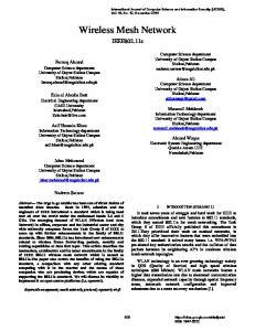
We compare the performance of Distributed Spatial Aggregation Tree (DSAT) scheme with shortest hop tree (SPT) scheme. Figure 4 shows the variation of the aggregate fair throughput as the number of sources is increased from 2 to 10. Each point on the graph is an average of 20 experiments, and in each experiment, the sources are selected randomly from the grid and the peak throughput for CBR traffic calculated for the DSAT and SPT. The average distance of the sources from the sink is 5 hops. DSAT does not give much improvement over SPT for two sources, because as stated before, merging two flows doesn’t have any advantage over two contending flows, and most instances in a random sample either cannot be spatially separated, or are already spatially separated in the SPT. DSAT starts showing better performance over SPT as the number of sources is increased and there is more option for early merging. Figure 5 shows the variation of the peak aggregate fair throughput with increase in the average path length of the flows. For each case, five sources are chosen randomly at a particular distance from the sink, and the peak aggregate fair throughput is calculated for the two routing strategies. When the sources are just one hop away, all the links contend with each other, and DSAT does not give any improvement with respect to SPT. As the sources are moved away from the sink, or the CAN, the difference between DSAT and SPT becomes visible. An interesting point is when the average hop length increases from 1 to 2, the SPT causes a decrease in the aggregate throughput because there are more links being used which contend with each other, whereas DSAT causes an increase in aggregate throughput because it is possible to spatially separate these paths and reduce contention. The figures show that DSAT routing improves the capacity of the network by separating out the paths and merging them when they interfere with each other. The throughput improvement is 10-15%. The aggregate throughput in both graphs denote the capacity of the network which remains largely unaffected by the number of sources or the path length. B. Fair rate allocation In Figure 6, we show how we do flow control to arrive at the fair throughput value for each flow if there are multiple sources in the network. We use a binary search method starting with an initial load of 2Mbps and the minimum and maximum load set to 0 and 4Mbps respectively. Then if the maximum loss rate for the flows is less than 5%, we increase the minimum load, while we decrease the maximum load otherwise. This is done until the difference between the minimum and maximum becomes less than 10Kbps. In this experiment, we choose 3 sources at an average distance of 7 hops from the sink, and do flow control to arrive at the peak fair throughput for the flows. The figure indicates clearly that the peak throughput obtained

Max. aggregate throughput (Kbps)

A. Evaluation of DSAT routing

1800

DSAT SPT

1600 1400 1200 1000 800 600 400 200 0 2

3

4

5

6

7

8

9

10

No. of sources

Fig. 4. Peak aggregate fair throughput of flows vs Number of Flows. Average path length of each flow is 5 hops.

1800 Max. aggregate throughput (Kbps)

network and packets missing deadlines, some frames cannot be reconstructed by the codec. The number of these missing frames depends on the capacity of the network and the constructed tree, as well as the delay budget.

DSAT SPT

1600 1400 1200 1000 800 600 400 200 0 2

3

4

5

6

7

8

9

Average path length

Fig. 5. Peak aggregate fair throughput of flows vs Path length. There are 5 flows in the network.

for DSAT is at around 310 Kbps, while for SPT, it is about 250 Kbps. Figure 8 shows how the loss rate varies with the increase in load. It can be observed that in DSAT, a lower loss rate can be maintained until much higher load, and even if the load is increased beyond that, the loss rate is around 20-30% lesser in DSAT from SPT. We realized that the method of flow control described above does not utilize the network capacity in the best possible way. The flow which attains the least maximum throughput decides the bit rate of every other flow. So, we implemented a modification to the above scheme where we try to provide the residual available bandwidth to the flows, which have not attained their maximum yet. We keep increasing the load on each flow until one flow reaches its maxima. This is done until each flow has reached its local maximum. Whenever one flow reaches its maximum, its load is fixed and is not increased further. Figure 7 shows how DSAT can help achieve a much higher aggregate throughput than SPT using this scheme. While the earlier figures show that DSAT helps attain a higher max-min throughput, this figure shows that once the max-min stage is reached, you can still increase the load of other flows at no cost to other flows using DSAT. On the other hand, in a shortest path tree, although the aggregate throughput can be increased, it will be at the cost of some flow.

6

100

DSAT SPT

400

Max loss rate for a source

Min throughput of a source (Kbps)

500

300

200

100

DSAT SPT

80

60

40

20

0

0 0

500

1000

1500

2000

0

500

Load (Kbps)

Fig. 6. Maximum of the minimum throughput among three flows vs Offered Load. SPT 1 SPT 2 SPT 3 SPT Agg. DSAT 1 DSAT 2 DSAT 3 DSAT Agg.

1000 800

2000

SPT DSAT DSAT + ED DSAT + ED + RR DSAT + ED + RF DSAT + ED + RR + RF

80 Packet delivery ratio

Throughput (Kbps)

1200

1500

Fig. 8. Minimum of the maximum loss among three flows vs Offered Load. 100

1400

1000 Load (Kbps)

600

60

40

400 20 200 0 0

100

200

300

400

500

600

700

Load (Kbps)

Fig. 7. SPT 1, 2 and 3 denote the throughput for flows 1, 2 and 3 in a shortest path tree as the load is increased to their local maximum. SPT Agg. denotes the aggregate throughput for shortest path tree. Similarly DSAT 1, 2 and 3 denote the throughput for 3 flows in Distributed spatial aggregation tree and DSAT Agg. shows the aggregate throughput.

C. Evaluation of other optimizations In this section, we evaluate the improvement obtained by the early dropping technique, the packet reordering schemes, and their combinations. The following acronyms are used to denote these optimizations – ED denotes Early Drop, RR denotes packet reordering based on residual delay budget, and RF denotes packet reordering based on the instantaneous throughput predicted for the flow. The instantaneous throughput is predicted by counting the number of packets transmitted in the previous 2 seconds for each flow. The packets of the flow, which has been sending a lesser number of packets in the previous time windows is given preference in the current time window. The three sources from the previous experiment are configured to send video traffic. The bit rate of the video and the delay budget is varied in the experiments. The following experiments show results for one of the sources. Figure 9 shows the variation of packet delivery ratio as the bit rate of the video traffic is increased for each source. The delay budget is fixed at 2.5 seconds. SPT experiences a large number of losses compared to DSAT because the average packet delay is greater than 2.5 seconds. As the bit rate is increased, the flow also starts to suffer from losses in the network, and so the delivery ratio decreases even further. DSAT increases the capacity of the network by spatially separating the paths, but still experiences losses due to the delay in the network. Early Drop increases the packet deliv-

0 200

250

300

350

400

Video Bit Rate (Kbps)

Fig. 9. Packet delivery Ratio vs Bit Rate of Streaming Video. Graph compares SPT, DSAT and the enhancements in DSAT. Delay Budget = 2.5s.

ery ratio to up to 20% at high bit rates, while packet reordering increases the packet delivery ratio by another 15%. This is reflected in the percentage of frames that can be reconstructed as shown in Figure 10. At a bit-rate of 300Kbps, DSAT can reconstruct 30% more frames than SPT, and further optimizations help in reconstructing 30% more frames. Figure 11 shows the variation of packet delivery ratio with the increase in delay budget. The bit rate is fixed to 300 Kbps. An infinite buffer at the receiver end will eliminate all losses, but it is not practical. Through this experiment, we demonstrate that if the network has the knowledge of the delay budget, it can help reduce losses using the optimizations stated. Figure 12 shows the variation of the percentage of frames which can be successfully reconstructed as the delay budget is increased. Its interesting to see that if the delay budget is equal to 2.5 seconds which is about the same as the path latency, and the bit rate is 300Kbps, almost all the frames can be reconstructed with DSAT and optimizations, while in SPT, just 20% of the frames can be reconstructed. Packet losses and missing frames lead to a decrease in PSNR values of the frames in the video. Figure 13 compares the PSNR values of the first 150 frames of the video for SPT, DSAT, DSAT with all optimizations, and a reference PSNR value assuming no losses. It is interesting to see that DSAT gives an improvement of over 2-3 db, while the optimizations improve the PSNR values to almost the reference value, which is a further increase of 7-8 db.

7

Percentage of frames reconstructed

100

VI. C ONCLUSIONS

SPT DSAT DSAT + ED DSAT + ED + RR DSAT + ED + RF DSAT + ED + RR + RF

80

60

40

20

0 200

250

300 Video Bit Rate (Kbps)

350

400

Fig. 10. Frames correctly reconstructed vs Bit Rate of Streaming Video. Delay Budget = 2.5s. 100

SPT DSAT DSAT + ED DSAT + ED + RR DSAT + ED + RF DSAT + ED + RR + RF

Packet delivery ratio

80

60

40

20

0 0.5

1

1.5

2

2.5

3

Delay Budget (s)

Fig. 11. Packet Delivery Ratio vs Delay Budget. Video bit rate = 300Kbps.

Percentage of frames reconstructed

100

SPT DSAT DSAT + ED DSAT + ED + RR DSAT + ED + RF DSAT + ED + RR + RF

80

60

40

20

0 0.5

1

1.5 2 Delay Budget (s)

2.5

3

Fig. 12. Frames Correctly Reconstructed vs Delay Budget. Video bit rate = 300Kbps. 40

Reference PSNR SPT DSAT Optimized DSAT

35 30

PSNR

25 20 15 10 5 0 0

20

40

60

80

Frame Number

Fig. 13. PSNR vs frame number

100

120

140

We have presented a wireless mesh architecture for efficient and cost effective transport of video streams from multiple surveillance cameras to a central monitoring station. We have addressed the two key requirements, high bandwidth and low delay jitter, for supporting good quality video over mesh networks. We proposed the construction of a distributed spatial tree that merges flows from video sources that are closely located while spatially separating those that are far apart. We provide fairness among the flows by limiting the rate of all video streams to the best achievable rate. We designed several optimizations for the mesh routers to reduce the delay jitter. Our results show that the improvement in the video quality is significant(7-10 dB) with all the optimizations and validates the design of Ganges Architecture. R EFERENCES [1] Networking Research Group, Microsoft Research. http://research.microsoft.com/mesh. [2] A. Raniwala, K. Gopalan, and T. Chiueh, “Centralized channel assignment and routing algorithms for multi-channel wireless mesh networks,” SIGMOBILE Mob. Comput. Commun. Rev., vol. 8, no. 2, pp. 50–65, 2004. [3] MIT Roofnet. http://www.pdos.lcs.mit.edu/roofnet. [4] V. Navda, A. Kashyap, and S. R. Das, “Design and evaluation of iMesh: An infrastructure-mode wireless mesh network,” in Proceedings of IEEE Int. Symp. on a World of Wireless, Mobile and Multimedia Networks (WoWMoM 2005), (Taormina, Italy), pp. 164–170, June 2005. [5] S. Mao, S. Kompella, Y. Hou, H. Sherali, and S. Midkiff, “Routing for multiple concurrent video sessions in wireless ad hoc networks,” in Proceedings of the 2005 IEEE International Conference on Communications (ICC), (Seoul, Korea), May 2005. [6] Y. Li, S. Mao, and S. S. Panwar, “The case for multipath multimedia transport over wireless ad hoc networks.,” in BROADNETS, pp. 486–495, 2004. [7] W. Wei and A. Zakhor, “Multipath unicast and multicast video communication over wireless ad hoc networks.,” in BROADNETS, pp. 496–505, 2004. [8] E. Setton, X. Zhu, and B. Girod, “Congestion-optimized multi-path streaming of video over ad hoc wireless networks.,” in ICME, pp. 1619– 1622, 2004. [9] R. Punnoose, P. Nikitin, and D. Stancil, “Efficient simulation of ricean fading within a packet simulator,” in Proceedings of IEEE Vehicular Technology Conference (VTC 2000), pp. 764–767, 2000. [10] B. R. J. Klaue and A. Wolisz, “Evalvid - a framework for video transmission and quaity evaluation,” in In Proc. of 13th International Conference on Modelling Techniques and Tools for Computer Performance Evaluation, Urbana, Illinois, USA, September 2003. [11] K. Chih-Heng, “How to evaluate mpeg video transmission using the ns2 simulator.” http://hpds.ee.ncku.edu.tw/˜smallko/ns2/Evalvid in NS2.htm.