Real-time visual astronomy using image intensifiers and Data Modeling Holger M. Jaenisch*a, William J. Collins**b, James W. Handley*a, Alex Hons***c, Miroslav D. Filipovic***c, Carl T. Case*a, and Claude G. Songy*a a
SPARTA, Inc., bCollins Electro Optics LLC, cUniversity of Western Sydney
Keywords: Data Modeling, image intensifier, astronomy, real-time imaging, image enhancement
ABSTRACT This paper presents the use of an image intensifier as an astronomical eyepiece for real-time observation of deep sky objects. The optical frequency spectra of observational astronomical objects are reported and compared with the spectral response curve of a Generation 3 intensified optical system. Image intensifier performance on various classes of deep sky objects is also reported along with methods for performing real-time image enhancement.
1. INTRODUCTION Image intensifier tubes have been in existence for over 40 years and have been both militarily and commercially applied successfully to terrestrial viewing and navigation applications in low light surroundings. These tubes take the minutest hint of illumination and transform the deepest shadows of darkness into well-lit scenes1. Because of these successes, we attempt to use image intensifiers to view meteors, galaxies, stars, clusters, and nebulae of the night sky.
2. ASTRONOMICAL SPECTRA AND THE IMAGE INTENSIFIER 2.1. Galactic spectra It is generally agreed that the spectral range of human vision is between approximately 380 to 760 nanometers (nm). The A curve (Fig. 1) represents the spectral response of a typical ITT Night Vision Generation 3 intensifier used in the I3 PIECE2. One can immediately see that the tube response extends to 900 nm with the peak near 775 nm. This region of the spectrum between 760 and 900 nm is included in the near infrared portion of the electro magnetic spectrum and is not visible to the eye in real time without the assistance of a device such as an image intensifier. Curve B (Fig. 1) is a fitted plot of galaxy types (spiral, elliptical, irregular). The slope of Curve B is a good fit to tube response of Curve A, particularly between 550 and 800 nm. The majority of spectral output falls above 700 nm and extends to 900 nm with good uniformity. Although galactic spectra extend well beyond 900 nm, this work only covers the spectrum of tube operation < 900 nm. It should also be noted that the spectrum of Curve B actually begins below the threshold of sensitivity of curve A. Generation 3 devices are essentially blind to this (violet) portion of the visible spectrum, but this narrow band between 400 and 450 nm represents a small percentage of the entire galactic spectra that is visible.
*
[email protected]; ph 1 256 337 3768; fax 1 256 830 0287; http://www.sparta.com; 4901 Corporate Dr., Suite 102; Huntsville, Alabama, USA 35805; **
[email protected]; ph 1 303 889 5910; http://www.ceoptics.com; 9025 E. Kenyon Ave.; Denver, Colorado, USA, 80237; ***
[email protected]; Intl. phone 61 2 47360135; local phone (02) 47360135; Intl fax 61 2 47360129; http://www.uws.edu.au/astronomy/index.html; Astronomy, School of Engineering and Industrial Design, University of Western Sydney, Locked Bag 1797, PENRITH SOUTH DC, NSW 1797, AUSTRALIA.
Curve B represents the average spectrum of the entire galactic mass for the three galaxy types. Within individual galactic types, the spectrum and the intensifier response can be further quantified. Ellipticals, which are classified by Hubble category from E0 (round) to E7 (elliptical), are symmetrical in shape. M87 is an example of an elliptical. The stellar population of ellipticals is called Population 1 from the work of Walter Baade at the 100 inch Mount Wilson Telescope. Ellipticals in fact are comprised of "old" Population 1 stars. Ellipticals are "metal rich", are predominately M Class, and include red giants, most of which exceed 10 billion years in age. From a spectral standpoint, ellipticals are very energetic sources in the red and infrared portions of the spectrum. Ellipticals display a uniform spectral curve across their entirety and when taken individually, their spectra are similar to the S2 curve of Fig. 1 (an M Class star). This far red/infrared spectrum makes ellipticals an excellent match to the image intensifier response (Fig. 1, Curve A). Spiral galaxies can be normal (Hubble Type S) or barred (Hubble Type SB). Both types are also classified A, B, or C, depending on the tightness of spiral structure that they display, with A being tightest and C being most open. Also the size of the nucleus relative to the spiral structure is from the largest (A) to the smallest (C). Some galaxies show disk like structure without spiral structure and are termed S0. Within the nucleus of spiral types, old Population 1 stars predominate as in ellipticals. The nuclear bulge is therefore also an excellent match for the intensifier spectral response. As we look into the spiral structure, gas, dust and young (Population 2) stars are most prominent. This makes the spiral structure more skewed towards the blue portion of the spectrum, hence making the spiral structure less visible using image intensification than the nuclear central bulge. This can be confirmed observationally by noting the increase in luminosity between the nuclear and the spiral structure. The image intensifier response to the spiral structure independent from the nuclear bulge is very dependent on the averaged spectrum that comprises the entire spiral structure. To clarify this important point, spiral galaxies that present their structure to us without oblique perspective such as M101 will appear highly intensified in the nucleus and will show little difference from visual observation in their spiral structure due to the predominately blue response in the spiral arm region. As the observer’s plane of view to the galaxy becomes more oblique, the dust lanes become more prominent. Galaxies such as M107 and NGC 4565 present an "edge on" appearance. The dust lanes have a strong infrared signature making these galaxy types ideal for imageintensified observation. Irregular galaxies have Hubble classifications of IRR1 (mostly O and B type stars and HII regions) with a general lack of dust clouds, and IRR2 (not resolvable into stars, no HII regions) with prominent dust lanes. Of these two, IRR2 types have a more red/infrared spectrum (dust lane infrared signature) and may be a better match to the intensifier spectral sensitivity. Two additional galaxy types not easily classified are Seyfert (1 and 2) and BL Lacertae objects. Both Seyfert types have unusually small and optically intense (star like) nuclei. Of the two types, Seyfert 2 has a more energetic infrared spectrum. BL Lacertae objects have rapid intensity variations in visible and infrared wavelengths and may be a good candidate for image-intensified observation. 2.2. Stellar Spectra Curve S1 (Fig. 1) is a star with spectral class G such as our sun or Capella. It is significant to note that the distribution of spectral energy lies with the majority in the visible spectrum and decreases (although still significant) in the infrared. These ‘main sequence’ stars have surface temperatures of approximately 5000 ˚K producing the spectral distribution curve of S1. Looking at Curve S2 in Fig. 1, we see a spectral distribution shifted more towards the red-infrared portion of the spectrum. This would fall into spectral class M that includes red supergiant stars such as Betelgeuse in Orion or Anteres. M stars excellently match the spectral response of the imaging tube. M stars have surface temperatures in the 3000 ˚K range causing their red shifted spectrum. Spectral class types B, A, and F are not shown. These hotter and bluer stars have spectra shifted towards blue and ultraviolet (the spectral region at the 400 nm end of Fig. 1). These star types may show modest or no intensity increase when viewed with a Generation 3 intensifier due to their spectrum falling in the region near the tubes minimum response. K types fall between G and M and are also not shown. Understanding where a star’s spectral class falls within the intensifiers effective spectral range (curve A in Fig. 1) will allow the user to predict effectiveness from an image intensification standpoint. M giants and supergiants give the greatest potential for image-intensified observability. 2.3. Nebulae The most predominate frequency for nebulae is centered at the HII line in Fig. 1, Curve D. This is the H-alpha line at 656.32 nm and is the result of spontaneous photon emission from the ionized hydrogen gas present in the nebula as
electrons decay from the 3rd to 2nd energy level. Other gases present within the nebula may also be ionized, as is the case with the great nebula in Orion (M42) in which ionized helium and oxygen are also present. These optical recombination lines give rise to other characteristic spectra causing emission lines at other wavelengths. In the case of M42, ionized oxygen at 500.7 and 495.9 nm produces the green light present with HII emission producing the greater part of the red emission. Emission nebulae will show greatly enhanced observability using Generation 3 intensification when most of their emission spectra occur within the HII region; the first emission line in the Balmer series of hydrogen emission lines. As electrons decay from higher valence levels within the hydrogen atom, they emit photons at higher frequencies. This gives rise to the Balmer series of visible emission spectra with the first line (known as hydrogen alpha or HII). There are 5 emission lines in the Balmer series that are present in the visible spectrum at 656 nm, 486 nm, 434 nm, 410 nm, and 397 nm. We can predict the image intensified observability of emission nebulae by first knowing what ionized gasses constitute their observable spectra and their corresponding emission line frequencies. These emission lines can then be plotted in relation to the tube response curve and their potential for amplification predicted. As with emission nebulae, the ionized spectra present are due to their proximity to a star(s), and in the case of planetary types, their surrounding a hot star (30,000 to 100,000 ˚K). The Ring Nebula in Lyra is a good example with a characteristic circular shell (hence planetary by Herschel) surrounding the central star with a temperature of 70,000 ˚K. The strong ionizing radiation gives rise to hydrogen (Balmer series) and oxygen lines at 500.7 and 495.9 nm. The shell of expanding gas in M57 is an excellent choice for Generation 3 intensification because of its HII abundance and to a lesser extent its oxygen lines. The central star, although observable with intensification, is nevertheless very blue in color and at the low end of the intensifier response. The observability of planetary nebulae is based on the identical criteria previously stated for emission nebulae. Certain nebulae are simply clouds of dust that are illuminated by nearby stars and reflect the stellar spectra present. The Pleiades are a good example of a reflection nebula in the presence of young (hot, blue) stars. The nebulosity present in the cluster reflects the blue spectrum present in these stars. The potential for intensified observability can be determined by the characteristic spectrum of the stars that illuminate reflection nebulae. 2.4. Visual vs. silicon based spectral sensitivity One of the first things that the astronomer notices when using an image intensifier is that the image is green. Using Table 1, it can be seen that at 505 nm, the minimum threshold of perceptible vision for green light is 1, yellow light requires 100 times the intensity to produce the equivalent visual response, orange 1000x, red incredibly 10000x, blue 2x and violet 20x. This visual spectral sensitivity is based on scotopic (rod vision). During photopic (cone) vision (light levels above approximately 10 LUX), the peak sensitivity shifts upwards to 555 nm. The image intensifier phosphor screen spectral frequency is centered at 530 nm. With the phosphor screen output illumination level at 2.25 foot lamberts maximum, the visual response falls within the threshold region between scotopic and photopic visual sensitivity. Therefore, 530 nm represents the ideal median frequency for the typical level of visual adaptation that occurs when using a Generation 3 image intensifier. Also and very importantly, as the intensifier illumination level drops (when imaging low surface brightness galactic objects for example), the eyes response becomes predominantly scotopic and the perception of color will actually disappear because of the retinal rods insensitivity to color and the visual transition to gray scale. Therefore, the green image present at higher illuminated image levels will become less apparent as the objects level of illumination decreases to the point of showing little or no color as the tube output approaches the equivalent background illumination (EBI) of the tube. Green frequency phosphor also greatly reduces the power requirement necessary by the tubes power supply because of the much greater visual sensitivity to green 530 nm light which in turn, extends the operating hours with a given (battery) power source. Color
Red
Orange
Yellow
Green
Blue
Violet
Wavelength nm
670
605
575
505
470
430
Relative Radiant Power
10,000
1,000
100
1
2
20
Table 1: Relative radiant power of light for different wavelengths (colors). It requires 10,000 times more radiant power of red than green light to cross a minimum perceptibility threshold.
In Fig. 1, the peak spectral response of the tube is at 775 nanometers. The ‘gain’ of the tube (output illumination divided by input illumination) is independent from photo response. The gain setting for the Generation 3 tube is 50,000. This gain is present across the spectrum of photo response. This brings us to one of the most important concepts concerning the use of a Generation 3 intensifier for astronomical objects: the ability to dynamically amplify the optical spectrum of a star, nebula or galaxy is directly related to the integrated spectrum of the object. The same statement applies to human vision except that the peak response is literally at the other end of the spectrum. An excellent example of the differences between visual and intensifier response is apparent with SC galaxy types such as M33. The naked eye response does not give the appearance of the galaxy nucleus as being brighter than the spiral arms to the magnitude that is actually measured with instrumentation with bolometric response. This is due to the eye responding with much greater sensitivity to the spiral arm section made up of much bluer stars than the nucleus which, although much more energetic than the spiral arms, is nevertheless comprised of much older red M class stars and large HII regions to which the eyes response is much less sensitive to (Fig. 1). The intensifier responds in a much more linear fashion in comparison to the eye, and therefore provides a more accurate response to astronomical objects over a large portion of the spectral response of human vision as compared to the eye over the same spectral range.
3. REAL-TIME IMAGING AND ENHANCEMENT 3.1. Collins Electro Optics I3 intensified eyepiece The ITT NIGHT VISION Generation 3 Image Intensifier tube in the I3 PIECE (center, Fig. 1) amplifies the light focused on its input window from the telescope. The telescope image is amplified or intensified by approximately 50,000 times. The amplified image is displayed on the rear or output end of the tube called the phosphor screen, which can be seen when the optical attachments are unthreaded from the rear of the tube housing. It is this greatly amplified image that is coupled to the human eye, a 35mm camera, a CCD camera, or video camera. Using the I3 PIECE adapter is very straightforward; all of the attachments are threaded to match the I3 PIECE adapter thread on its output end. All attachments have a stop or locating ring to facilitate their focal point location when removed and reattached3. From a light gathering standpoint, the I3 PIECE makes any telescope perform as if it were both lower in f number and larger in aperture. The image quality is excellent with sharp star images across the full field of the eyepiece. Many amateur astronomers have reduced visual acuity when their eyes are dark adapted (scotopic vision). This is unfortunate since our vision needs to be at its best during extended observing sessions, and in reality our eyes may not perform well for a number of reasons. The I3 PIECE makes extended duration viewing comfortable with an eye relief of 1.5" (using the supplied 25 mm eyepiece) and immediate image acquisition without the need for holding a steady eye position. There is far less dark adaptation time required when using the I3 PIECE as compared to conventional optics, with typical adaptation to the tube image under dark sky conditions occurring in 30 seconds or less. With a signal to noise ratio of up to 25 db, background noise is reduced to a minimum. The image background displays minor scintillation (amplifier) noise when operated in telescopes at f15 and above. Object brightness versus the background sky brightness (contrast) is fundamental to the success of using image intensification technology for astronomy. Historically, this has been a shortcoming of attempting to use low signal to noise ratio, low resolution intensifiers for visual astronomy because they produce such a noise filled image that the contrast difference between the deep sky object and the sky is reduced to nearly zero. High signal to noise ratio and high photo response in the I3 PIECE makes it possible to see subtle details in many deep sky objects that would be invisible with conventional optics. High urban levels of sky glow combined with increased humidity will reduce the visible contrast difference between astronomical objects and the sky to zero for all but the brightest starts, some planets, and the moon. Under these conditions, the I3 PIECE will make many objects visible, particularly star clusters, oblique galaxies (such as NGC 4565), and many nebulae that are not visible or are marginally visible with conventional optics at very low contrast levels. It should be noted that an important difference between the I3 PIECE and a standard CCD camera is that the I3 PIECE is a real-time device while a CCD camera is not. The image on the I3 PIECE phosphor screen is useable optically without any interface, whereas the CCD must gather light over some period of time and requires a computer interface. The CCD camera actually has greater sensitivity to low light but over a much greater period of time. Many astronomers who use an
image intensifier for the first time complain that they are disappointed with the resolution using words like grainy and low-resolution. This, however, is not the case with the image intensifier. In fact, in terms of detail in objects (resolution) that can be seen using the I3 PIECE, the tube is capable of displaying resolutions up to 64 line pairs per millimeter, that is .00062 inches or .016 mm per line pair. (There are 1120 line pairs across the 18 mm phosphor screen.) In comparison with a CCD camera, most commercially available CCD cameras have pixel sizes between 9 and 18 microns (.009 mm to .018 mm). If we use critical sampling (the Nyquist limit), which is 2 pixels across the resolution element, then we have .018 to .036 mm for our minimum sample. The image intensifier resolution is .016 mm per pair (equivalent to 16 micron pixels for a CCD), making individual element resolution of the image intensifier output phosphor screen comparable with high-end CCD camera performance. The graininess of images is taken care of through the use of much lower noise Generation 3 tubes. Any further apparent graininess is due to the short persistent phosphor used in the image intensifier and the inability of the eye to integrate the real-time image. Close examination of Fig. 2 shows that although the graininess of each of the five images decreases going from left to right, the resolution remains constant in each of the five frames. However, as the integration time changes (increases moving from left to right), the graininess dissolves into the average image that we are conditioned to seeing with our eyes. If longer persistence phosphor were used, graininess in the image would also disappear, however, image blur would begin to occur. Depending on the user application, a trade of image intensifier phosphor persistence versus graininess and image blur may reveal that an image intensifier with a medium persistence that yields frames much like the middle frame in Fig. 2 is preferred. 3.2. Archer Real-time Video Enhancer Video enhancers such as the one produced by Radio Shack (shown in Fig. 3) are one method for real-time controllable image enhancement and background removal on images captured from an image intensifier. This unit has adjustments for Fade, Video Noise Reduction (VNR), Comparator, and Enhancement as well as two sets of RCA input and outputs for both video and audio connections, and TV/VHF/RF connectors are located on the rear panel. The frequency response at –3 dB is between 25 Hz-2.2 mHz, at greater than +3 dB is .25-3.0 mHz, and at greater than + 12db is .42-2.2 mHz. This enhancement hardware allows the user to increase or decrease the brightness and contrast of the image in real-time. The Enhancement adjustment works much like an Embossing spatial convolution operator or kernel in raising the stellar image while leaving the background at a lower value and giving the appearance that the image is being illuminated from a specific compass point direction. Mathematically, this is given by -1 0 1 -1 k= 11. -1 0 1
(1)
where k is the convolution kernel operator4. An example of this is shown in Fig. 3, where the image on the left (raw image of stars in M51 Whirlpool Galaxy) is enhanced using the hardware in the center to the image on the right, where noise can now be eliminated leaving just the stars in M51. 3.3. Recursive Frame Averaging Removal of the graininess and transient noise in image frames can be accomplished easily and efficiently in hardware in real-time as the images are being collected with the image intensifier using a recursive frame averager. The recursive frame averager dramatically reduces background noise while increasing SNR. Collins reports that the averager reduces the SNR by up to 9 db3. The user can select 0, 2, 4, 8, or 16-frame averaging. For example, if 16-frame averaging is selected, 16 frames are taken initially of the scene, averaged together, and the average frame displayed. Once this initialization process is done, the frame averager then performs frame averaging and displays output in real-time streaming fashion. This is done in hardware by deleting the oldest frame in the averager, bumping each of the remaining 15 frames stored in the averager up one buffer, and receiving the current video frame from the telescope. Once the buffer is again filled, an average frame is generated and the process repeated. This frame averaging process removes transient noise that does not appear at the same location from frame to frame. When 8 or 16 frame averaging is selected, noise reduction is so dramatic that the sky background becomes very smooth and optically ‘quiet’ with very little observable noise. Fig. 2 shows output from the frame averager for 0, 2, 4, 8, and 16 frame averaging. It should be noted that the image on the left (0 averaging) shows how relatively noisy each of the input frames were to the frame averager, but due to the random nature of the noise, it was averaged away with increased number of frames to average.
3.4. Image enhancement using Data Modeling Jaenisch has proposed and demonstrated the applicability of Data Modeling for processing raw images for robust autocontrast adjustment. Data Modeling does not require the use of dark field or flat field subtraction, uses only the measured image captured from the image intensifier, and provides visually pleasing images where other auto-balancing techniques fail. This method constructs a mask that isolates the background from the object of interest, and works as long as there is contrast between the object and background. If the object is of lower value than the background, a negative is generated to make the object have higher values than the background. The first step of this process is usually to add the original image (A) to itself one or more times until the edge of the object of interest in the image becomes saturated to 255. (B). This ensures that the object itself is saturated. Once this is done, the original (A) is then subtracted from this saturated intermediate image (B) to create a new intermediate (C). This subtraction causes the values of the object in C to become low, and the background to have higher values. The values of the background in this image (C) are compared to the values of the background in the original (A) to insure that they are equivalent or of higher value. If condition is not currently met, this intermediate image is added to itself the number of times required to meet this condition. Once met, the intermediate image (C) is subtracted from the original image (A) to yield the final enhanced image. It should also be noted that once C is generated, if desired areas of the object are not low enough in value, additional subtractions of the original image from C may be necessary to insure both that the object has enough contrast with the background and that the background of C is greater than or equal to the value of the background of the original. As an equation, this can be represented as B=A+A C=B–A . D=A-C
(2)
where A is the original image, B and C are intermediate steps, and D is the final processed image. A flowchart of this is shown in Fig. 4. Attempts to reduce the mathematical complexity of this algorithm by combining individual steps into one destroys the process due to the inherent image saturation, thresholding, and renormalization that exists at each step in the process. Examples of this process are discussed in further detail in Section 4 and are shown in Fig. 7 and 8. 3.5. STV by Santa Barbara Instrument Group (SBIG) Santa Barbara Instrument Group (SBIG) has developed a hybrid design that combines traditional video technology and cooled integrating CCD camera technology for video imaging and autoguiding called the STV (shown in Fig. 5). Video cameras use uncooled camera chips and generally allow no longer than 1/30th of a second exposures. Because of its unique design, the STV allows exposures from as small as 1/1000th of a second all the way up to 600 seconds. The STV video output can be viewed on the built-in LCD display or on any external video monitor. SBIG estimates the STV will reach 14th magnitude stars with one-second integrations through an 8" SCT, and 18th magnitude in 60 seconds5. It should be noted that the STV has an actual camera size of 656 x 480 pixels, but operates in three different binning modes (656 x 480 binned 3 x 3, 640 x 400 binned 2 x 2, and 320 x 200 binned 1 x 1). Section 4 discusses an example of an image taken with the STV shown in Fig. 9. 3.6. Determination of R0 (seeing) using the STV Astronomical “seeing” is usually expressed in arc seconds, and is a measure of the minimum separation distance between the two stars in a double star that can be resolved. This can be accomplished by applying a two hole mask to an 8 or 10-inch aperture telescope. The mask simulates two telescopes 8 inches apart using only one telescope. On most nights, the seeing is poorly correlated, even over this short separation. If one had a perfect drive, the jiggle of one star image about its average position is mathematically related to the seeing. If the two images are essentially uncorrelated, then the relative motion of one star image to the other is 1.4 times the motion of a single image to the average location. This relative separation, though, is insensitive to drive errors since the images move together and both are affected in the same manner by the drive errors. By calculating the relative separation between the two, the drive error is subtracted out. This technique is called Differential Image Motion Monitor (DIMM). An accurate seeing measurement with the DIMM technique as implemented in the STV requires a bright star high in the sky, and low wind speeds. The short exposure is required to not attenuate the stellar motion. For example, if each
exposure was several seconds long on a turbulent, windy night, the stellar image centroids would move very little – the movement all takes place at shorter time scales. The STV uses exposures from 2 milliseconds up to 100 milliseconds. If the wind speed is below 4 miles per hour the measurement should be good always. With a bright star, wind speeds up to 30 mph should be tolerable. Mathematically, the long exposure FWHM in arc seconds is given by FWHM = 0.98 * λ/(4.85x10-6* R0).
(3)
where λ is the wavelength in cm (0.00006) and R0 is the atmospheric cell size in cm. R0 is the transverse phase coherence length (commonly called the Fried parameter), and most textbooks describe it as being on the order of 3 to 4 inches (7.5 to 10 cm). It is related to the rms differential image motion by R0 = {rms2/[2* λ2*(0.179*d-1/3 – 0.0968*r-1/3)]}-3/5.
(4)
where d is the individual aperture diameter in cm, r is the separation of apertures in cm, and rms is the standard deviation of spot separation in cm. The equation and methodology has been tested by numerous investigators and found to give accurate results. With great optics and an excellent mount, the FWHM of a long exposure image will be the value determined by the STV seeing monitor. Typically some blurring is contributed by each source, but the better the mount and optics, the less the contribution of the first two terms is to the aggregate FWHM. The aggregate FWHM is given by FWHM (Aggregate) = [FWHM2(optics) + FWHM2(fast drive error) + FWHM2(seeing)]1/2.
(5)
Where the FWHM (Aggregate) is what is measured by the STV and is made up of FWHM from the optics, drive error, and seeing. For this reason, the result is approximate. DIMM is demonstrated in Fig. 5 (right). On this particular night, the two images of the object using the DIMM process were separated by an amount varying between 0 arc seconds and at most approximately 6 arc seconds. At this instant in time, the two images were separated as shown in the top and isometric views on the top of the figure. The movement (dancing) of the two object images is due to instabilities in the seeing5.
4. EXAMPLES Fig. 6 shows the relative utility of image intensifiers. A low resolution (320 x 200) Casio QV-10 camera was used to capture a meteor burning up upon entry into the Earth’s atmosphere at approximately 3:00 AM CST on November 18, 2001 during the Leonids meteor shower. Jaenisch captured this series of images with the image intensifier using 1/30th second exposure with 5 seconds delay between each frame. Both the image intensifier and the camera were hand-held in this application using eyepiece projection. The Data Modeling algorithm given in Section 3.4 was applied to M51 in Fig. 7, where the original image was taken in Track and Accumulate mode with the STV and a dark frame subtracted from each frame before accumulation. Background effects present in the image are due to readout noise and sky glow, both of which are not handled with flat field and dark field subtraction. Data Modeling, however, corrects for these effects well, and does not require even initial dark field and flat field subtraction to be performed. Using the 3rd frame captured in Fig. 6, Jaenisch applied the novel background detection and subtraction algorithm given in Section 3.4 to extract the meteor, its tail, and other stars in the area (Fig. 8). This processing did an excellent job, but required an extra step to achieve each of the algorithm criteria. Fig. 9 provides five images labeled A-E for comparison. I3 PIECE images are higher resolution (> 3000000 pixels) than STV images (64000 pixels) and were cropped for display; however, all images are shown at their original resolutions. Image A is M13 taken with the STV using a single 5-second exposure and shows the lack of resolution of this device (320 x 200). This is contrasted with B, another image of M13 taken using an AP 7” f9 refractor and the I3 PIECE by removing the eyepiece from the I3 PIECE and imaging the photocathode directly. Image C is an STV image of M42, using the Track and Accumulate function and eight (8) ten second exposures while the STV autoguided the telescope.
This 320 x 200 resolution image is contrasted with D, which was taken with a 10” Meade LX200 SCT f3.3 using the Collins Electro Optics I3 PIECE and eyepiece projection. This image was captured by the camera directly thru the 25mm eyepiece that comes standard with the I3 PIECE, and represents what the image looks like visually to the observer looking into the I3 with the naked eye. Image E was taken using the same equipment setup as Image B, and shows an excellent example of the photo quality imagery that is possible with an image intensifier. It should be noted here that none of the graininess or lack of resolution complained about by astronomers can be seen, confirming what was mathematically proven earlier in this work in Section 2.5 that the I3 PIECE is actually equivalent in resolution to good CCD cameras on the market. Fig.10 shows the limiting magnitude of two different optical systems using the I3 PIECE. On the left, a AP 7” f9 refractor and Canon D30 camera were used to characterize M57 with a system limiting magnitude of 16.1. On the right, a Meade LX-200 10” SCT f6.3 using a Sony DSC F707 camera and eyepiece projection were used to characterize M67 with a system limiting magnitude of 14.56,7.
5. FUTURE WORK AND CONCLUSIONS The authors have shown in this work the applicability of image intensifiers to real-time astronomy. Specifically, the Collins Electro Optics I3 PIECE has removed many of the problems of the past in this technology area with increased resolution that is better even than most CCD cameras, and reduced noise in the intensifier tube using Generation 3 technology to remove graininess. This technologically advanced hardware could be taken one step further to provide a simple real-time method for removing the background from any image using the autonomous contrast adjustment Data Modeling algorithm described above in Section 3.4. This algorithm could be implemented in firmware and performed in real-time before the image intensifier tube displays the final image output to the eyepiece or camera, and does not require the use of a dark frame or bias frame. The same is true of the STV; the algorithm could also be integrated into its firmware to allow automatic contrast adjustment of background saturation instead of just providing dark frame subtraction. In addition, this autonomous contrast adjustment algorithm can be applied to the frequency domain of an image, where a simple inverse mask can be constructed autonomously that isolates high contrast points, and then removes them when an inverse frequency transform is applied and the image is transformed back to the spatial domain. Depending on the user application, a trade of image intensifier phosphor persistence versus graininess and image blur may reveal that an image intensifier with a medium persistence is preferred. Coupling of the I3 PIECE with the STV provides a robust real-time tool for astronomers and investigators interested in enhanced object imagery and viewing.
ACKNOWLEDGMENTS The authors would like to thank the faculty, staff, and students involved in the Astronomy Internet Masters (AIM) program at the University of Western Sydney for their advice and support, and M.P. Carroll and S.K. Roberts, TecMasters, Inc. (TMI) for their encouragement. Also, the authors would like to express their gratitude to K. Kurtts for the support given to them during this work, and Falco, Marcel, Marcus, and Alynnde Jaenisch for their help in collecting the Leonid meteor shower data.
REFERENCES 1) di Cicco, D. “Intensifying Your Viewing Experience”, S&T, pp. 63-66, February, 1999. 2) ITT Industries, “ITT Night Vision”, http://www.ittnv.com, June 1, 2002. 3) Collins, W. “Collins Electro Optics – Image Intensified Astronomy”, http://www.ceoptics.com, June 1, 2002. 4) Berry, R. and Burnell, J., The Handbook of Astronomical Image Processing, Ch 4, 12-13, Willmann-Bell, Richmond, VA, 2000. 5) Santa Barbara Instrument Group, “SBIG Santa Barbara Instrument Group”, http://www.sbig.com, May 23, 2002. 6) Martinez, P. and Klotz, A., A Practical Guide to CCD Astronomy, pp. 214-216, Cambridge University Press, Cambridge, 1998. 7) Gupta, R. Observer’s Handbook 2002, pp. 56-57, University of Toronto Press, Toronto, Ontario, Canada, 2001.
FIGURES
Fig 1: Typical spectral response curve for the Generation 3 intensifier used in the I3 PIECE (left) and typical spectral response curve for spiral, elliptical, and irregular galaxies (right).
Fig 2: Result of frame averaging using from left a) 0 frames (raw), b) 2 frames, c) 4 frames, d) 8 frames, and e) 16 frames. Note that resolution is the same in all 5 frames.
Fig 3: Result of video enhancement using Radio Shack Archer Video Processor Model #151272A (center). Image on left is a measured star field in M51, and on the right is the same star field pulled out of the noise background with the video processor.
A = raw image
B=A
Obj. saturation
C= B+A
Y
E= C-A
Bkgnd. D > Bkgnd. A
D= E
N B=C
Y
F=A - D
N E= D+ D
Fig 4: Flow of Data Modeling algorithm developed by Jaenisch for image enhancement and background subtraction using only the raw image itself.
Fig 5: STV by Santa Barbara Instrument Group (left) and an example calculation of astronomical seeing using the STV.
Fig 6: Leonids meteor shower captured with an image intensifier and a low resolution (320 x 200) Casio QV-10 camera with 1/30 sec exposure with 5 sec between each frame. Both the image intensifier and the camera were hand-held in this application using eyepiece projection.
Fig 7: Application of the autonomous auto-contrast adjustment Data Modeling algorithm to M51.
Fig 8: Data Modeling required more steps to both raise background and lower object in mask construction as mandated by the criteria given in Fig. 4.
Fig 9: Images collected using the I3 PIECE and eyepiece projection and the SBIG STV.
Fig 10: Limiting magnitude of two different optical systems using the I3 PIECE.