A title page comment if desired — not to appear in the publication.
Astronomy in the Cloud: Using MapReduce for Image Coaddition K. Wiley, A. Connolly, J. Gardner and S. Krughoff
arXiv:1010.1015v1 [cs.DC] 5 Oct 2010
Survey Science Group, Department of Astronomy, University of Washington
[email protected] and M. Balazinska, B. Howe, Y. Kwon and Y. Bu Database Group, Department of Computer Science, University of Washington ABSTRACT In the coming decade, astronomical surveys of the sky will generate tens of terabytes of images and detect hundreds of millions of sources every night. The study of these sources will involve computation challenges such as anomaly detection and classification, and moving object tracking. Since such studies benefit from the highest quality data, methods such as image coaddition, i.e., astrometric registration, stacking, and mosaicing, will be a critical preprocessing step prior to scientific investigation. With a requirement that these images be analyzed on a nightly basis to identify moving sources such as potentially hazardous asteroids or transient objects such as supernovae, these data streams present many computational challenges. Given the quantity of data involved, the computational load of these problems can only be addressed by distributing the workload over a large number of nodes. However, the high data throughput demanded by these applications may present scalability challenges for certain storage architectures. One scalable data-processing method that has emerged in recent years is MapReduce, and in this paper we focus on its popular open-source implementation called Hadoop. In the Hadoop framework, the data is partitioned among storage attached directly to worker nodes, and the processing workload is scheduled in parallel on the nodes that contain the required input data. A further motivation for using Hadoop is that it allows us to exploit cloud computing resources, i.e., platforms where Hadoop is offered as a service. We report on our experience implementing a scalable imageprocessing pipeline for the SDSS imaging database using Hadoop. This multi-terabyte imaging dataset provides a good testbed for algorithm development since its scope and structure approximate future surveys. First, we describe MapReduce and how we adapted image coaddition to the MapReduce framework. Then we describe a number of optimizations to our basic approach and report experimental results comparing their performance.
–2– Subject headings: image coaddition, Hadoop, cluster, parallel data-processing, distributed file system, SDSS, LSST
1.
Introduction
Many topics within astronomy require data gathered at the limits of detection of current telescopes. One such limit is that of the lowest detectable photon flux given the noise floor of the optics and camera. This limit determines the level below which faint objects, (e.g., galaxies, nebulae, and stars), cannot be detected via single exposures. Consequently, increasing the signalto-noise ratio (SNR) of such image data is a critical data-processing step. Combining multiple brief images, i.e., coaddition, can alleviate this problem by increasing the dynamic range and getting better control over the point spread function (PSF). Coaddition has successfully been used to increase SNR for the study of many topics in astronomy including gravitational lensing, the nature of dark matter, and the formation of the large structure of the universe. For example, it was used to produce the Hubble Deep Field (HDF 1999). While image coaddition is a fairly straightforward process, it can be costly when performed on a large dataset, as is often the case with astronomical data (e.g., tens of terabytes for recent surveys, tens of petabytes for future surveys.). Seemingly simple routines such as coaddition can therefore be a time- and data-intensive procedure. Consequently, distributing the workload in parallel is often necessary to reduce time-to-solution. We wanted a parallelization strategy that minimized development time, was highly scalable, and which was able to leverage increasingly prevelant service-based resource delivery models, often referred to as cloud computing. The MapReduce framework (Google 2004)offers a simplified programming model for data-intensive tasks, and has been shown to achieve extreme scalability. We focus on Yahoo’s popular open-source MapReduce implementation called Hadoop (Hadoop 2007). The advantage of using Hadoop is that it can be deployed on local commodity hardware but is also available via cloud resource providers (an example of the Platform as a Service cloud computing archetype, or PaaS ). Consequently, one can seamlessly transition one’s application between small- and large-scale parallelization and from running locally to running in the computational cloud. This paper discusses image coaddition in the cloud using Hadoop from the perspective of the Sloan Digital Sky Survey (SDSS) with foreseeable applications to next generation sky surveys such as the Large Synoptic Survey Telescope (LSST). In section 2, we present background and existing applications related to the work presented in this paper. In section 3, we describe cloud computing, MapReduce, and Hadoop. In section 4, we describe how we adapted image coaddition to the MapReduce framework and present experimental results of various optimization techniques. Finally, in sections 5 and 6, we discuss final conclusions of this paper and describe the directions in which we intend to advance this work in the future.
–3– 2.
Background and Related Work 2.1.
Image Coaddition
Image coaddition is a well-established process. Consequently, many variants have been implemented in the past. Examples include SWarp (SWarp 2002, 2010), the SDSS coadds of Stripe 82 (SDSS DR7 2009), and Montage (Montage 2010) which runs on TeraGrid (TeraGrid 2010). SWarp does support parallel coaddition; it is primarily intended for use on desktop computing environments and its parallelism is therefore in the form of multi-threaded processing. Parallel processing on a far more massive scale is required for existing and future datasets. Fermilab produced a coadded dataset from the SDSS database (the same database we processed in this research), but that project is now complete and does not necessarily represent a general-purpose tool that can be extended and reused. Montage most closely related to our work but there are notable differences. Montage is implemented using MPI (Message Passing Interface), the standard library for message-passing parallelization on distributed-memory platforms. MapReduce is a higher-level approach that offers potential savings in development time provided one’s application can be projected well onto the MapReduce paradigm. Hadoop in particular (in congruence with Google’s original MapReduce implementation) was also designed to achieve high scalability on cheap commodity hardware rather requiring parallel machines with high-performance network and storage. Image coaddition (often known simply as stacking) is a method of image-processing wherein multiple overlapping images are combined into a single image (see Figs. 1 and 2). The process is shown in Algorithm 1. First, a set of relevant images is selected from a larger database. To be selected, an image must be in a specified bandpass filter (line 6) and must overlap a predefined bounding box (line 9). The images are projected to a common coordinate system (line 10), adjusted to a common point spread function (PSF) (line 10), and finally stacked to produce a single consistent image (line 18).
2.2.
Experimental Dataset
Much of modern astronomy is conducted in the form of large sky surveys in which a specific telescope and camera pair are used to produce a consistent1 database of images. One recent and ongoing example is the Sloan Digital Sky Survey (SDSS) which has thus far produced seventy terabytes of data (SDSS DR7 2009). The next generation survey is the Large Synoptic Survey Telescope (LSST) which will produce sixty petabytes of data over its ten year lifetime starting this decade. These datasets are large enough that they cannot be processed on desktop computers. Rather, large clusters of computers are required. In this paper we consider the SDSS database. The SDSS camera has 30 CCDs arranged in a 1
A set of images with similar spatial, color, and noise statistics.
–4–
Algorithm 1 Coadd Input: {ims: one set of images, qr: one query} Output: {coadd: a single stacked, mosaiced image, depth: coadd′ s per-pixel coverage map} 1: tprojs ← empty // set of projected intersections 2: qf ← qr filter // bandpass filter 3: qb ← qr bounds 4: for each image im ∈ ims do 5: imf ← im filter 6: if imf = qf then 7: imb ← im bounds 8: twc ← intersection of qb and imb // Get intersection in RA/Dec 9: if twc is not empty then 10: tproj ← projection of im to twc // Astrometry/interpolation/PSF-matching 11: Add tproj to tprojs 12: end if 13: end if 14: end for 15: coadd ← initialized image from qr 16: depth ← initialized depth-map // same dimensions as coadd 17: for each image tproj ∈ tprojs do 18: Accumulate tproj illumination into coadd 19: Accumulate tproj coverage into depth 20: end for
–5–
.*-/0 1232/
'()*# '+",-
'()*# '+",-
!"#$%&
!"#$%&
@2
=>6$"/5
?-6 .*-/0 42*(56
AB-/3")&
AB-/3")&
@2
=>6$"/5
?-6 7/28-$#9 #2912"55
7/28-$#9 #2912"55
!"#$%9 7:;
!"#$%9 7:; :#"$
74GF4#HG@49I6?$##J##K;@?H49$#94L:I47#IH6#M56;I4G4@
Fig. 7.— Coadd Running Times (shorter bars are better) — Two queries (large on left, small on right) were run via three methods (from left to right: prefiltered FITS input, non-prefiltered unstructured sequence file input, prefiltered structured sequence file input). We observe that the second and third methods yielded 5x and 10x speedups relative to the first method for the large query. Note that the number of mapper input records (FITS files) for the three methods for the large query was 13415, 100058, and 13335 respectively.
– 17 –
Table 1. Coadd Running Times (minutes) For Two Query Sizes Method
1◦
1/ ◦ 4
Raw FITS input, not prefiltereda Raw FITS input, prefiltered Unstructured sequence file input Structured sequence file input, prefiltered SQL → unstructured sequence file input SQL → structured sequence file input
315.0 42.0 9.2 4.0 7.8 4.1
194.0 25.9 4.2 2.7 3.5 2.2
a This
method was not explicitly tested. The times shown were estimated by assuming linearity (see section 4.1.1 for justification) and scaling the second method’s running time by the prefilter’s reduction factor (7.5), e.g., 42.0×7.5 and 25.9×7.5.
– 18 – Fig. 8 shows a breakdown of the prefiltered job’s overall running time for the larger query into the salient stages. The last bar represents the total running time, 42 minutes, the same measurement indicated in the first bar of Fig. 7. A call to main() involves a preliminary setup stage in the driver followed by a single call runJob() which encapsulates the MapReduce process. Thus, the bar in the fourth region is the sum of the bars in the first and third regions. Likewise, the call to runJob() runs the MapReduce process and has been further broken down into the components shown in the second region. Thus, the bar in the third region is the sum of the bars in the second region. We observe that the dominating step of the overall process is Construct File Splits. This indicates that the Hadoop coadd process spent most of its time locating the FITS files on HDFS and preparing them as input to the mappers. The cost associated with this step results from a set of serial remote procedure calls (RPCs) between the client and the cluster. The actual image-processing computations are represented only in the two shortest bars labeled Mapper Done and Reducer Done indicating that Hadoop spent a small proportion of its total time on the the fundamental task. This observation suggests that there is substantial inefficiency in the associated method, namely in the RPCs involved. The next section describes one method for alleviating this problem. We never explicitly measured the performance without prefiltering but an estimate is easy to calculate. Given that the running times with prefiltering for our two experimental query sizes were 26 and 42 minutes respectively and given that the running time was dominated by the serial RPC bottleneck and given that the prefilter reduced the number of input files by a factor of 7.5 (about 13,000 files out of the 100,000 total passed the prefilter), we can estimate that without prefiltering, the process would have taken approximately 194 and 315 minutes respectively (Table 1, first row). This estimate assumes a linear relationship between the number of files to be found on HDFS and the required time, which is justified given that the number of RPCs is constant per file and the amount of time required per RPC is constant.
4.1.2.
Optimizing Hadoop with Sequence Files
While Hadoop is designed to process very large datasets, it performs better on a dataset of a given size if the total number of files is relatively small. In other words, given two datasets of identical data with one dataset stored in a large number of small files and the other stored in a small number of large files, Hadoop will generally perform better on the latter dataset. While there are multiple contributing factors to this variation in behavior, one significant factor is the number of remote procedure calls (RPCs) required in order to initialize the MapReduce job, as illustrated in the previous section. For each file stored on HDFS, the client machine must perform multiple RPCs to the HDFS namenode to locate the file and notify the MapReduce initialization routines of its location. This stage of the job is performed in serial and suffers primarily from network latency. For example, in our experimental database we processed 100,000 files. Each file had to be independently located on HDFS prior to running the MapReduce job and this location
– 19 –
"25C#2
7.*8#9+3#
2+):&';
@>
?>
>
!
!"#$
8 2+):& 7.** 1&)0 ';< #2!"& #9+3#2!" *+,!- ,2+3,!45%#! & ) ) # # 6*%5,0 .,/0 !"#$$%&'(")*
%&'!()
=.5)
;
/(#* ?%65*%()* '6/&5"@:*440
9:
9;
9< -78+*-./(
+(,&("'(*-./(* 01$121#(*+$%&'$&%()* 23*415(%1*46/&5"* 1")*46/6%
Fig. 9.— Sequence Files — A sequence file (each column) comprises a set of FITS files (layers). We convert a database of numerous FITS fits to a database of fewer actual files (sequence files) using one of two methods. The first method has no structure (top). FITS files are assigned to sequence files at random. The second method maps the SDSS camera’s CCD layout (see Fig. 3) onto the sequence file database, i.e., there is one sequence file for each CCD on the camera. FITS files are assigned accordingly and thus a given sequence file contains FITS files of only one bandpass and from only one column of the Camera.
– 22 – However, it is also worth considering a more rationally motivated sequence file structure since doing so might permit pruning, i.e., filtering as demonstrated above. We refer once again to Fig. 3 which shows the SDSS camera’s CCD layout. This time, we use the SDSS camera’s CCD arrangement not to define a prefiltering method on FITS files, but rather to impose a corresponding structure on the sequence file database. We define 30 distinct sequence file types, one corresponding to each CCD of the camera (see Figs. 3 and 9). Thus, a given sequence file contains only FITS files originating from one of the original 30 CCDs. If the sequence files are named in a way which reflects the glob filter described previously, we can then filter entire sequence files in the same way that we previously prefiltered FITS files. This method of filtering permits us to eliminate entire sequence files from consideration prior to MapReduce on the basis of bandpass or column coverage of the query. We anticipated a corresponding improvement in performance resulting from the reduction of wasted effort spent considering irrelevant FITS files in the mappers. Table 1 (row four) and Fig. 7 (third bar in each set) show the results of using structured sequence files and prefiltering in concert. We observe a further reduction in running time over unstructured sequence files by a factor of two on the larger query. The savings in computation relative to unstructured sequence files resulted from the elimination of much wasted effort in the mapper stage considering and discarding FITS files either whose bandpass did not match the query or whose sky-bounds did not overlap the query bounds. Both prefiltering methods suffer from false positives resulting from the fact that the spatial filter occurs on only one spatial axis. Likewise, the non-prefiltered method performs no prefiltering at all. Therefore, in all three methods, effort is still being wasted considering irrelevant FITS files. The prefiltering methods processed 13,000 FITS files in the mappers while the non-prefiltered method processed the entire dataset of 100,000 FITS files. However, the number of FITS files that actually contributed to the final coadd was only 3885. In the next section we describe how we used a SQL database and query prior to running MapReduce to eliminate this problem.
4.1.4.
Using a SQL Database to Prefilter the FITS Files
All three methods described previously (prefiltered FITS files, unstructured sequence files, and prefiltered structured sequence files) process irrelevant FITS files in the mappers. Toward the goal of alleviating this inefficiency, we devised a new method of prefiltering. This method consists of building a SQL database of the FITS files outside of HDFS and outside of Hadoop in general. The actual image data is not stored in the SQL database — only the bandpass filter and sky-bounds of each FITS file are stored, along with the necessary HDFS file reference data necessary to locate the FITS file within the sequence file database, i.e., its assigned sequence file and its offset within the sequence file. Running a job using this method consists of first performing a SQL query to retrieve the subset of FITS files that are relevant to the user’s query, and from the SQL result constructing
– 23 – a set of HDFS file splits 5 to specify the associated FITS files within the sequence file database (See Fig. 10). The full set of file splits then comprises the input to MapReduce. The consequence of using SQL to determine the relevant FITS files and sending only those FITS files to MapReduce is that this method does not suffer from false positives as described above. Thus, the mappers waste no time considering (and discarding) irrevelant FITS files since every FITS file received by a mapper is guaranteed to contribute to the final coadd. The intention is clearly to reduce the mapper running time as a result. Table 2 shows the number of FITS files read as input to MapReduce for each of the six experimental methods. Note that prefiltering is imperfect, i.e., it suffers from false positives and accepts FITS files which are ultimately irrelevant to the coaddition task. However, the SQL methods only process the relevant files.
5
Although the concept of a file split is complicated when one considers the full ramifications of storing files on a distributed file system, it suffices for our discussion to define a file split simply as the necessary metadata to locate and retrieve a FITS file from within a host sequence file.
– 24 –
&'( !)*)+),% !"#73%*"#%$%7 89:&7;%,7 *?)*7.$%"


![Hyrax: Cloud Computing on Mobile Devices using MapReduce [PDF]](https://m.moam.info/img/260x300/hyrax-cloud-computing-on-mobile-devices-using-mapr_648f03c1098a9e69678b456f.jpg)