common classification results in binary and non-binary vox- elization approaches. The latter can be further divided into filtered [30] [27], multivalued voxelization ...
Real-time Voxelization for Complex Models Zhao Dong Wei Chen Hujun Bao Hongxin Zhang Qunsheng Peng State Key Lab of CAD&CG, Zhejiang University, 310027, Hangzhou, China {flycooler, chenwei, bao, zhx, peng}@cad.zju.edu.cn
Abstract In this paper we present an efficient voxelization algorithm for complex polygonal models by exploiting newest programmable graphics hardware. We first convert the model into three discrete voxel spaces according to its surface orientation. The resultant voxels are encoded as 2D textures and stored in three intermediate sheet buffers called directional sheet buffers. These buffers are finally synthesized into one worksheet, which records the volumetric representation of the target. The whole algorithm traverses the geometric model only once and is accomplished entirely in GPU (graphics processing unit), achieving real-time frame rate for models with up to 2 million triangles. The algorithm is simple to implement and can be integrated easily into diverse applications such as volume based modelling, transparent rendering and collision detection.
1. Introduction As an alternative to traditional geometric representation, the volumetric representation plays an important role in computer graphics community since the 1980s. It provides a uniform, simple and robust description to synthetic and measured objects and founds the basis of volume graphics [19]. Conceptually, a reformulation process is required to generate volumetric representation from geometric object. This stage is typically called voxelization. It accomplishes the conversion from a set of continuous geometric primitives to an array of voxels in the 3D discrete space that approximates the shape of the model as closely as possible. This concept was first introduced by Arie Kaufman [20] [18]. Since then its applications in diverse fields have been broadly explored, including volume modelling [31], virtual medicine [21], haptic rendering [22], visualization of geometric model [32], CSG modelling [10], collision detection [13] [2] [11] and 3D spatial analysis [1] etc. There are many strategies to conduct voxelization. Basically, they can be classified as surface voxelization [5]
[28] [16] and solid voxelization [27] [12] methods. Another common classification results in binary and non-binary voxelization approaches. The latter can be further divided into filtered [30] [27], multivalued voxelization [8] [15], object identification voxelization [16] and distance transform [26] [29]. As the form of processed primitives is concerned, there are methods for line [4], triangle [5], polygon [20] [30] [17], CSG [10], parametric surface [18] [27] and implicit surface [28] voxelization. Concerning the structure of the volume, the result can be stored in the form of regular grid [31], general 2D lattices [26] or distance transform [33]. Most previous work focuses on the sampling theory involved in voxelization and rendering. By introducing welldefined filters in the stages of voxelization and reconstruction, the rendering quality is greatly improved. However, due to the rapid development of the modelling and sensor technologies, the size and complexity of the models are even larger. This puts high demands on the performance of the voxelization algorithm, especially for time-critical applications such as virtual medicine, haptic rendering and collision detection. Most of researchers rely on standard graphics systems for fast voxelization. However, to our best knowledge, achieving real-time frame rate for a moderate size volume resolution is still a challenge. Thanks to modern graphics hardware [23] [24], its powerful flexibility and programmability enlight us to overcome the problems in an alternative way. This paper describes a novel real-time voxelization approach for polygonal surfaces as well as solid and multi-valued voxelization. We decompose the task into three stages, namely, rasterization, texelization and synthesis which are accomplished entirely in GPU (graphics processing units). The resultant volume is represented as one or multiple 2D textures in video memory which can be reused conveniently. With mainstream graphics card, it can convert millions of triangles or complex deformable models into a 2563 volume at 10 fps or even real-time. The rest of this paper is organized as follows. Section 2 gives a brief review of related works. The voxelization al-
gorithm is outlined in section 3. The implementation details are described in section 4. Section 5 presents our preliminary efforts to extend the fundamental algorithm to a flexible and configurable voxelization engine. Experimental results and technical discussions are given in section 6. Conclusions and future work are addressed in section 7.
2. Previous Work The research focus of voxelization in 1990s were mainly on modelling aspects such as robustness and accuracy. In 1993, S.Wang et al. [30] proposed voxelization filters and normal estimation for accurate volume modelling. Many efforts [28] [16] [27] were later introduced for improving the rendering quality by using enhanced normal vector estimation schemes and smoothing filters. In addition, Dachille and Kaufman [5] presented an efficient approach for incremental triangle voxelization. Recently, Haumont and Warzee [12] proposed a solid voxelization method by means of a 3D seed-filling approach. Widjaya et al. [33] accomplished the voxelization in general 2D lattices, including hexagonal lattices and 3D body-centered cubic lattices. More recently, Varadhan et al. [29] applied the max-norm distance computation algorithm to determine whether the surface of a primitive intersects a voxel. Attentions have also been paid on the performance improvement. One effective way is to exploit the data coherence and workload distribution in a shared memory multiprocessor [25]. As voxelization is basically a 3D scan conversion process, it is natural to make use of rasterization graphics hardware in parts of or the whole voxelization pipeline. The slicing-based voxelization algorithm presented in [3] generates slices of the underlying model in the frame buffer by setting appropriate clipping planes and extracting each slice of the model. These slices constitute the final volume. The algorithm was later extended to a wide range of 3D objects [8] [9] [10] and applications including 3D spatial analysis [1] and collision detection [2]. However, its algorithmic complexity is proportional to the slice number of the resultant volume. Likewise, the technique presented in [6] projects the object to six faces of its bounding box through standard graphics system for the outermost parts and read back the information from depth buffer. Its main disadvantage lies in the convexity requirement of the processed model and hence restricts its usages. Based on the concept of depth peeling [7], Heidelberger et al. [15] [14] presented an effective algorithm for fast layered depth image (LDI) generation that can be extended to voxelization. Though the algorithm achieves relative accurate results, its performance is dominated by the scene complexity and the scene depth complexity. And the accessed depth-lists need to be sorted by CPU at each frame.
Typically, there are three deficiencies for graphicshardware-accelerated voxelization algorithms. First, the performance decreases greatly following the increase of the scene complexity and the volume resolution since the model is traversed multiple times. Second, the access of frame buffer demands high bandwidth between main memory and video memory, which is still a heavy bottleneck in modern graphics hardware. Third, the voxelization results are directly stored in color or depth buffer and cost lots of video memory. Therefore, it is difficult to afford interactive frame rate at the volume resolution of 256×256×256. The algorithm presented in this paper aims to address these three issues using programmable graphics hardware, i.e, the algorithm complexity, the amount of the data transfer and the storage/usage of the result volume.
3. The New Voxelization Algorithm Without loss of generality, we present the algorithm by instancing triangular mesh models in this section. It can easily be adapted to general surface models by slightly changing the voxelization pipeline.
Figure 1. Illustration of the voxelization of a triangle.
A triangular mesh model T is usually represented as a sequence of vertices with their positions, normals and texture coordinates associated with a list of indices that form each triangle. Assume a regularly sampled volume P of 2L ×2M ×2N voxels with spacing d be defined in the bounding box B of the model. A voxel pijk stands for voxelized values including occupancy, density, color and gradient (Figure 1). The input of voxelization is T and its output is an array of attributed voxels pijk (i = 0...L − 1, j = 0...M − 1, k = 0...N − 1).
3.1. The Key Idea In the standard rasterization hardware, triangles are scanconverted into a 2D frame buffer. Only the frontmost frag-
ments are kept in the frame buffer storing the rasterization results. Whereas, voxelization is a 3D rasterization procedure and hence a discrete voxel space is required. The voxel space consists of an array of voxels that store all voxelized values. It can be represented as 2D or 3D textures in graphics hardware. Since writing directly to 3D texture is not supported in mainstream graphics card of PC platform, we choose to encode the volume in 2D texture. We call the texture worksheet as it records all voxelization information. Note that each texel in the graphics card typically consists of four components for red, green, blue and alpha channels respectively. Depending on the bit-depth of each voxel, one texel can represent one or multiple voxels. For instance, an 8-bit red component can store 8 voxels for binary voxelization. The conversion from volume space to worksheet invokes an encoding procedure called texelization. The storage of worksheet equals the size of the volume. For example, one 2048×2048 texture with four components is sufficient for binary voxelization at the resolution of 5123 . Note that the width and length of a worksheet may be very large and it might be divided into multiple patches. Each patch has the same width and length as that of the volume which corresponds to a slab of the volume along some axis direction (Figure 2). In high volume resolution cases, multiple worksheets are needed. To simplify the explanation, we suppose that one worksheet is used in following sections. Worksheet
cept and is not explicitly represented. In order to add a voxel to the worksheet, a blending operation is carried out at corresponding location. When all triangles are processed, the worksheet encodes the discrete voxel space. The 2D rasterization in standard graphics hardware involves a 2D linear interpolation process. If a triangle is parallel to the rasterization direction, the interpolation process results in a line segment in the discrete voxel space. Therefore, a triangle should be rasterized along the direction that is most parallel to its orientation. And three directional sheet buffers are used as intermediate space during the rasterization and texelization procedures. Each sheet buffer represents a part of the discrete voxel space. After these sheet buffers are accomplished, an additional reformulation process is performed to transcode them to the final worksheet (Figure 3). In this stage, each element is first transformed to the discrete voxel space and then encoded to the appropriate texel in the worksheet. Actually, the worksheet reformulates the slabs of the volume along a desired axis direction.
2D to 3D
2D to 3D
Sheet buffer along X
Sheet buffer along Z
3D to 2D
2D to 3D
Discrete Volume Space Slab
Composited Worksheet
Slab
Sheet buffer along Y
Patch Slab Slab
Figure 3. Synthesis of three directional sheet buffers.
Volume
Figure 2. The worksheet versus the slabs of the volume.
To sum up, the voxelization algorithm consists of three stages as follows. • Rasterization The triangles are rasterized to the discrete voxel space.
The conversion from the triangles to the discrete voxel representation can be accomplished in programmable graphics hardware. The volume is generated slab by slab. In other words, the worksheet is filled patch by patch. For each slab, only the triangles that intersect the slab are processed. Each chosen triangle is rasterized against an axis direction along which it has the maximum projection area. The position of each voxel is transformed to its 3D volume coordinates immediately. These coordinates are used to find the correct position in the worksheet. Note that, the discrete voxel space is only a virtual con-
• Texelization Each voxel is encoded and accumulated in some directional sheet buffer. • Synthesis Three sheet buffers are transcoded to the worksheet representing the final volume.
3.2. Voxel Access The simplest representation of voxelization is binary encoding that represents the occupiness of the triangles in the voxel space. Since each voxel is mapped into the set of
(0, 1), one bit is used for a voxel. For multivalued voxelization, more bits or bytes are required. For example, we can store the vector quantized normals, texture coordinates or colors in two, four bytes or even more bytes. It is also possible to encode the object identification or material identification. Suppose that the resolutions of the volume and worksheet are 2L ×2M ×2N and 2W ×2H respectively. Therefore 2L ×2M ×2N =2W ×2H ×C where C is the number of voxels encoded in a texel. For instance, C equals 32 for binary voxelization if a texel is composed of four 8-bit components. The numbers of patches along x and y axis are 2W −L and 2H−M . During rasterization, each patch corresponds to a volume slab and is placed in the worksheet orderly. To render the volume, a list of proxy rectangles is built like 2D slicing-based volume rendering. Every patch of the worksheet is then fetched and texture mapped to consecutive layers of rectangles. Since one element of each patch might encode multiple voxels, an efficient method to store and fetch a voxel within the worksheet is required. Accounting for this, four lookup operations are designed. Suppose the volume coordinates of the voxel are (px, py, pz). First, the corresponding patch is determined by dividing pz with C. Thereafter, the texel in the (px, py) is accessed from the found patch. Then, bit offset of correct component is decided again by pz and C. Finally, a lookup table facilitates accessing bits from a component.
3.3. Solid Voxelization The algorithm described above is designed for surface voxelization. To perform solid voxelization for closed objects, a 3D scan-filling operation similar to the 2D scanfilling algorithm is required to fill voxels of the inner region of the object. It traverses the volume slice by slice and line by line in a slice. Voxels on each scan line are checked from left to right. A flag is set for each scan line to indicate if the current voxel is inside the object or not. The flag is initially set to false and it changes its value when the scan line spans a voxel that intersects the boundary of the object. To eliminate the errors caused by singular points, we perform scan-filling along three axis directions and then check their common voxels.
• Dynamic Vertex and Index Buffers Putting the geometric data in AGP memory and updating them dynamically do not pay large performance penalty. • Multiple Render Targets In shader program, four render targets can be used simultaneously. • Dependent Texture Fetching The accessed texel value can be used to fetch another texture in the shader program.
4.1. Dynamic Index Buffer Updating As stated in section 3, the triangles are rasterized against three directions depending on their orientations. An expensive way is to traverse all the triangles of the model three times and rasterize them to different worksheets by comparing their surface normals in shader program. Alternatively, a preprocess can be performed to classify the geometric primitives into three groups according to their surface normals. Note that, the classification need be done only once for static models. If the model is deformable, the classification should be conducted by updating the dynamic index buffer that locates in Accelerated Graphics Port (AGP) memory. The fast transfer speed from AGP 8× to video memory makes the dynamic updating in real-time. Moreover, we can further divide the three groups into multiple smaller sets to avoid traversing the whole model for each volume slab. Each set bucket sorts the triangles that intersect the slab. Similarly, for deformable objects the intersection status of each triangle is checked dynamically. During the rasterization, two clipping planes are set along the slab borders to ensure accurate results. By means of multiple render targets, we can rasterize multiple slabs simultaneously, yielding better performance. In general, the performance penalty for dynamic index buffer is low. And the model is traversed approximately only once in rasterization stage.
4.2. Lookup Textures Many lookup textures are utilized in our implementation to replace the complex computation in shader program.
Programmable graphics hardware [23][24] makes the computation in GPU flexible and adjustable. In particular, our GPU supported algorithm exploits the following functionalities and features:
• Fetching One Bit One useful operation is to access one bit. To fetch the kth bit of an 8-bit component, we build a 256×8 lookup texture whose component is 0 or 1. Its (s, t) texel stores the value in the tth bit of s. A simple texture fetching instruction accomplishes the operation.
• Huge Texture Size The width and length of a texture can be 2048×2048. It provides enough space to keep a moderate size volume in the worksheet.
• Storing One Bit To store a bit into a component, an 8×1 texture is created. Its sth texel stores 2s . By setting the alpha blending operation as addition and the
4. Hardware Implementation
source/destination blending factors as one/one, the required bit value can be put at correct location during rasterization. • Worksheet Composition During the synthesis stage, three directional sheet buffers should be composited to one worksheet. This involves two transformations as illustrated in Figure 3. One is the transformation from 2D sheet buffers along different directions to 3D voxel space. The other transforms from the voxel space to the final 2D worksheet destination. To speed up these transformations, we build 2D textures that facilitate the lookup from the source coordinates to the destination coordinates. To compose the resultant volume along z-direction in the worksheet, we make two lookup textures that help mapping each location of the x and y direction sheet buffers to that of z direction sheet buffer, which is equivalent to the final worksheet. In fact, in most cases, one element of the worksheet corresponds to multiple consecutive voxels. And these voxels form a line in the other sheet buffers. Consequently, we need only build the lookup textures for the first voxel of each element of the worksheet. The locations of other voxels in the x,y directional sheet buffers can be obtained by offsetting operations in shader program. This scheme saves lots of memory in GPU.
ometric primitives from host applications. Its front/end interface converts the primitives to vertex arrays that will be handled directly. In many applications, only parts of models need be voxelized. The region of interests (ROI) could be determined rapidly by updating index buffer dynamically in CPU. Meanwhile, CPU accomplishes the normal-based classification and bucket sorting for polygonal models. The updated data is transferred through AGP port. In GPU, the classified geometric primitives are rasterized in a streaming mode. The results are encoded and stored as 2D textures in three direction sheet buffers. To render or access some patch of the textures, a common technique is to create a proxy rectangle and texture map the patch on it. In general, the proposed voxelization engine distributes the workload in CPU and GPU as outlined in Figure 4.
CPU Interfaces to Applications Geometry Proxy Geometry
Framebuffer Access
ROI Computation in AGP Geometry Array
4.3. Usages of the Resultant Volume Rasterization
Texelization
Synthesis
GPU
{
The resultant volume is represented as a worksheet in video memory, and hence consecutive access of the volume data are replaced by operating on 2D texture. For instance, rendering of the volume can be accomplished conveniently by accessing each internal voxel as described in Section 3.2. If multiple objects are to be manipulated, we can keep two resultant volumes as 2D textures simultaneously. Boolean operations can be done pairwise by means of several shader instructions. However, if the resultant volume has to be processed offline, a frame buffer read operation from video memory to host memory is required. The performance penalty is significant, especially for large size buffers. For 512×512 resolution, the transfer costs 75ms in our testing platform. Hence we recommend to use the volume in GPU directly.
Worksheets(2D Textures)
Applications: Solid Voxelization Volume-based Modelling Transparent Ilustrations Collision Detection
Figure 4. The proposed voxelization engine.
5. Applications of the Algorithm 4.4. Workload Distribution 5.1. Voxelization of Other Forms of Surfaces Since the operations on textures are convenient in the programmable context, the voxelization algorithm can be extended to geometric forms other than triangles as well as multipurpose volumetric manipulation tasks by slightly changing the pipeline. Three stages serve transparently for cumbersome voxelization and form an adjustable voxelization engine. The voxelization engine accepts a list of ge-
• Implicit Surface When host application computes the ROI of the target surface, we generate a sequence of rectangles embedded in the ROI and deal with them from front to back. We rasterize each rectangle to a render target. Every pixel in the render target represents a sampled point in 3D space. Its coordinates are
used to evaluate the implicit surface. If the result satisfies given conditions, the pixel is output and transformed to the worksheet subsequently. Generally, binary voxelization can be achieved by extracting the defined iso-surface while solid voxelization involves a procedure to find an interval that satisfies some inequation. Ideally, this method can handle very complex implicit surface given that the shader program supports enough long instruction slots. • Parametric Surface The rasterization of parametric surface is conducted in vertex shader instead of pixel shader. We build a boodle of points that cover the parametric field. Each point is considered as a vertex to be processed in vertex shader. Its texture coordinates in parametric domain are used to calculate the positions in 3D space. These positions are transcoded to the worksheet immediately.
handle arbitrarily-shaped geometries and the performance is dependent entirely on the volume resolution.
6. Results and Discussions Our experiments were carried out on a PC with a single 2.4 GHz Pentium IV CPU and 2GB RAM. An ATI Radeon 9800 Pro graphics card with 256MB RAM is equipped. All shader programs are written in Vertex/Pixel Shader 2.0 of Direct3D 9.0b version.
6.1. Performance
Transparent illustration has been an open problem in graphics community. Nevertheless, it becomes simple if rapid voxelization is feasible. Our initial attempt is based on the multivalued voxelization algorithm. Typically, we can choose to store the combinations of the vector quantized normals, texture coordinates and material identifications in the worksheet. By enabling the lighting in the rendering stage, the appearance of the model can easily shown. Furthermore, our voxelization engine can be integrated seamlessly into a slicing-based volume rendering. By rendering the volume data and voxelized slices orderly in 3D space, complex deformable geometric models are semitransparently shown in the volumetric scene. This technique is very promising in surgical planning, intra-operation navigation and radiation therapy.
Table 1 lists the voxelization performance in milliseconds for models at the volume resolution of 2563 . The respective images are illustrated in Figure 5 by assigning different colors. The voxelization timing consists of three parts, i.e, rasterization, texelization and synthesis. As the algorithm traverses the model approximately once, its performance is insensitive to the scene complexity. The rasterization timings depend on mainly the triangle numbers. For the Blade model with 1,765,388 triangles, it costs about 75 ms. On the other hand, texelization and synthesis are image space operations and their performances are dominated by the volume resolution and the bit-depth of voxel. In the 7th column, the preprocess timings for classifications are listed. It is also scene complexity-dependent. Note that, the dynamic updating for normal-based classification and bucket sorting take place only once for static models. In the last column, we report the normal surface rendering timings that depend on the scene complexity only. We do not list the performance of the visualization of the voxelized volume that depends mainly on the volume resolution and costs about 8 ms in average. We tested our binary surface voxelization algorithm for the Wagner model under different volume resolutions. The model has 60,246 triangles and 30,215 vertices. Timing statistics is reported in Table 2. To store the volume in one worksheet, we represent a voxel using one bit for 5123 resolution. It is clear that bit-operations are much more expensive than byte-operations. Specifically, we encode each vertex normal using 16 bits in 1283 resolution.
5.3. Collision Detection
6.2. Quality
Collision detection is a fundamental issue in many fields. We propose to transfer the intersection computation from geometric space to image space by our voxelization algorithm. We perform voxelization for the surfaces of the common parts of objects. Collision queries are carried out with 2D textures in image space. Since voxelization is no longer the bottleneck, the collision detection can reach real-time frame rate even for complex and deformable models. It can
The accuracy of the result is proportional to the volume resolution. Meanwhile, the bit-depth affects the performance as well as the consumed memory. If multivalued voxelization is required for high resolution volume, multiple worksheets are used given that there are enough video memory. If the blending operations for floating point textures are supported, less worksheets are needed and the performance will improve dramatically. At the moment, we
• CSG Models The voxelization of CSG model is straightforward. The nodes are first voxelized into respective worksheets. Then the constructions are done from bottom to top automatically in image space since boolean operations on 2D textures are well-defined by blending operations in GPU.
5.2. Transparent Illustration
Model Duck Hugo Bunny Dragon Buddha Blade
#Triangles 1,254 16,928 69,451 871,326 1,087,514 1,765,388
#Vertices 947 8,634 34,834 439,370 550,868 898,796
Rasterization 9.0ms 9.7ms 12.0ms 38.0ms 47.0ms 75.0ms
Texelization 8.0ms 8.3ms 8.0ms 8.0ms 7.8ms 8.0ms
Synthesis 10ms 10ms 11ms 11ms 10ms 12ms
Preprocess 0.8ms 7.0ms 27.0ms 330.0ms 415.0ms 660.0ms
Surface Rendering 0.7ms 0.8ms 1.3ms 10.8ms 13.5ms 20.8ms
Table 1. Voxelization timings for different model sizes. Volume resolution: 2563 , bit-depth: 8.
Resolution 5123 2563 1283 643
Bit-depth 1 8 16 8
Memory 16MB 16MB 4MB 256KB
Voxelization 500ms 30ms 24ms 21ms
Points 620,381 151,347 38,012 9,379
Result Rendering 240ms 10ms 6ms 4ms
Table 2. Voxelization of timings for Wagner model in different volume resolutions. conclude that 2563 resolution with 8-bit depth voxel is a good choice under current hardware conditions. To demonstrate the versatility of the voxelization engine, several preliminary experiments have been conducted. The left part of Figure 7 shows two images of surface and solid voxelization effects for an implicit surface (x4 − 5x2 + y 4 − 5y 2 + z 4 − 5z 2 + 11.8 = 0). Both of them take 25ms. In the right part of Figure 7, the voxelization effect of a transparent cerebra model with 36,758 triangles and 29,371 vertices is shown. After inserting it into an MRI head volume data with the resolution of 1283 , the intermixing effect is achieved by proposed hybrid volume rendering technique. The frame rate is about 10 fps. In our experiments, aliasing effects exist in solid voxelization for closed polygonal models. Prolonged lines appear where some voxels at the raterization stage are missing. This shows the gap and difference between software-based voxelization and graphics-hardware-accelerated algorithms.
6.3. Comparisons There are two typical graphics-hardware-accelerated methods, namely, the slicing-based voxelization [8] [9] and layered depth image (LDI) extraction [14]. However, there are two major differences. On one side, the slice-based voxelization method needs to rasterize the model the same times as the resolution of the volume along z direction. Though the results can be rendered to 3D textures as the algorithm proposed, this feature has not been supported in consumer graphics hardware of PC platform. Based on the experimental data reported in section 6.1, the slicing-based voxelization method costs about 5 sec-
onds (20.8ms × 256) for the blade model at the resolution of 2563 . On the other side, LDI approach reduces the traversal number to the scene depth complexity. It is view-dependent and is sensible to the model and needs to download the depth images from video memory. The depth lists have to be resorted pixel by pixel in CPU. Therefore, its efficiency is affected by the volume resolution greatly.
7. Conclusions and Future Work Fast or even real-time voxelization is essential for interactive graphics applications. We have presented a scheme to solve this problem by representing the resultant volume as 2D textures which can efficiently implemented. The approach is simple, robust and easy-to-implement. We believe it will be a useful tool in the near future with the rapid growth of graphics hardware performance. As future work is concerned, an important issue is the improvement of the voxelization quality, i.e, achieving separability, minimality robustness and accuracy simultaneously. The blending operations for floating point textures are available with the launching of NVidia Geforce 6800 Ultra. We would like to design more efficient voxelization algorithm based on it. It is also inspiring if the graphics card will provide 3D render target feature to avoid texelization operations. In addition, we intend to investigate enhanced voxelization algorithms for line, curve and comprehensive boundary representations such as point cloud models.
References [1] S. Beckhaus, J. Wind, and T. Strothotte. Hardware-based voxelization for 3d spatial analysis. In Proceedings of the 5th International Conference on Computer Graphics and Imaging, pages 15–20, Canmore, Alberta, Canada, August 2002. ACTA Press. [2] M. Boyles and S. Fang. Slicing-based volumetric collision detection. ACM Journal of Graphics Tools, 4(4):23–32, 2000. [3] H. Chen and S. Fang. Fast voxelization of 3d synthetic objects. ACM Journal of Graphics Tools, 3(4):33–45, 1999. [4] D. Cohen-Or and A. Kaufman. 3D line voxelization and connectivity control. IEEE Computer Graphics and Applications, 17(6):80–87, /1997. [5] F. Dachille and A. Kaufman. Incremental triangle voxelization. In Proceedings of Graphics Interface, pages 205–212, May 2000. [6] G. P. Evaggelia-Aggeliki Karabassi and T. Theoharis. A fast depth-buffer-based voxelization algorithm. ACM Journal of Graphics Tools, 4(4):5–10, 1999. [7] C. Everitt. Interactive order-independent transparency. Technical report, NVIDIA Corporation., May 2001. [8] S. Fang and H. Chen. Hardware accelerated voxelization. Computers and Graphics, 24(3):433–442, 2000. [9] S. Fang and H. Chen. Hardware accelerated voxelization. Volume Graphics, pages 301–315, 2000. [10] S. Fang and D. Liao. Fast csg voxelization by frame buffer pixel mapping. In Proceedings of the ACM/IEEE Volume Visualization and Graphics Symposium 2000, pages 43–48, Salt Lake City, UT, USA, October 2000. [11] N. Gagvani and D. Silver. Shape-based volumetric collision detection. In Proceedings of the IEEE Symposium on Volume visualization 2000, pages 57–61. ACM Press, 2000. [12] D. Haumont and N. Warzee. Complete polygonal scene voxelization. ACM Journal of Graphics Tools, 7(3):27–41, 2002. [13] T. He and A. Kaufman. Collision detection for volumetric objects. In Proceedings of IEEE Visualization 1997, pages 27–35. IEEE Computer Society Press, 1997. [14] B. Heidelberger, M. Teschner, and M. Gross. Real-time volumetric intersections of deforming objects. In Proceedings of Vision, Modeling, Visualization 2003, pages 461–468, Munich, Germany, November 2003. [15] B. Heidelberger, M. Teschner, and M. Gross. Volumetric collision detection for deformable objects. April 2003. [16] J. Huang, R. Yagel, V. Filippov, and Y. Kurzion. An accurate method for voxelizing polygon meshes. In IEEE Symposium on Volume Visualization, pages 119–126, 1998. [17] M. W. Jones. The production of volume data from triangular meshes using voxelisation. Computer Graphics Forum, 15(5):311–318, 1996. [18] A. Kaufman. Efficient algorithms for 3d scan-conversion of parametric curves, surfaces, and volumes. In Proceedings of ACM SIGGRAPH 1987, pages 171–179, USA, July 1987. ACM Press. [19] A. Kaufman, D. Cohen, and R. Yagel. Volume graphics. IEEE Computer, 26(7):51–64, 1993.
[20] A. Kaufman and E. Shimony. 3d scan-conversion algorithms for voxel-based graphics. In Proceedings of ACM Workshop on Interactive 3D Graphics, pages 45–76, Chapel Hill, NC, USA, October 1986. ACM Press. [21] K. Kreeger and A. Kaufman. Mixing translucent polygons with volumes. In Proceedings of IEEE Visualization 1999, pages 191–198, USA, October 1999. [22] W. McNeely, K. Puterbaugh, , and J. Troy. Six degree-offreedom haptic rendering using voxel sampling. In Proceedings of ACM SIGGRAPH 1999, pages 401–408, 1999. [23] Microsoft Corporation. DirectX 9.0 SDK, December 2002. [24] NVIDIA Corporation. Cg specification, August 2002. [25] C. E. Prakash and S. Manohar. Shared memory multiprocessor implementation of voxelization for volume visualization. HPC for Computer Graphics and Visualization, 17(3):135– 145, 1995. (Proc. Eurographics’98). [26] C. Sigg, R. Peikert, and M. Gross. Signed distance transform using graphics hardware. In R. Moorhead, G. Turk, and J. van Wijk, editors, Proceedings of IEEE Visualization 2003. IEEE Computer Society Press, October 2003. [27] M. Sramek and A. Kaufman. Alias-free voxelization of geometric objects. IEEE Transactions on Visualization and Computer Graphics, 5(3):251–267, 1999. [28] N. Stolte. Robust voxelization of surfaces. Technical Report TR.97.06.23, State University of New York at Stony Brook, 1997. [29] G. Varadhan, S. Krishnan, Y. J. Kim, S. Diggavi, and D. Manocha. Efficient max-norm distance computation and reliable voxelization. In Proceedings of the Eurographics/ACM SIGGRAPH symposium on Geometry processing, pages 116–126. Eurographics Association, 2003. [30] S. Wang and A. Kaufman. Volume sampled voxelization of geometric primitives. In Proceedings of IEEE Visualization 1993, pages 78–84. IEEE Computer Society Press, October 1993. [31] S. Wang and A. Kaufman. Volume-sampled 3d modeling. IEEE Computer Graphics and Applications, 14(5):26–32, 1994. [32] R. Westermann, O. Sommer, and T. Ertl. Decoupling polygon rendering from geometry using rasterization hardware. In Proceedings of the 10th Eurographics Workshop on Rendering, pages 53–64, 1999. [33] H. Widjaya, T. Mueller, and A. Entezari. Voxelization in common sampling lattices. In Proceedings of Pacific Graphics 2003, pages 497–501, Canmore, Alberta, Canada, October 2003.
Figure 5. Voxelization results for different models. Volume resolution: 2563 .
Figure 6. Voxelization results for Wagner model under different resolutions.
Figure 7. Applications of the voxelization engine.