Allen et al.19 demonstrated that laser beams with OAM have helical phase ...... Franke-Arnold S, Barnett SM, Padgett MJ, Allen L. Two-photon entanglement.
Realising high-dimensional quantum entanglement with orbital angular momentum Melanie McLaren1, 2, Filippus S. Roux2 and Andrew Forbes1, 2 1.
Laser Research Institute, University of Stellenbosch, Stellenbosch 7602, South Africa 2.
CSIR National Laser Centre, P.O. Box 395, Pretoria 0001, South Africa
Abstract We report the first quantum entanglement experiment in South Africa. The spatial modes of the entangled photon pair are investigated with their potential for highdimensional entanglement. The generation, measurement and characterisation of the entangled states are examined in detail, where we show high-dimensional entanglement in a Hilbert space of dimension 25. We highlight the experimental challenges contained within each step and provide practical techniques for future experiments in the quantum regime.
Introduction One of the most astonishing features of quantum mechanics is that of the entanglement of particles. First introduced as an objection to quantum mechanics by the famous Einstein, Podolsky and Rosen (EPR) thought experiment1, entanglement represents the notion of non-local quantum correlations between two or more quantum-mechanical systems. That is, for an entangled pair of particles the measurement of an observable for one particle immediately determines the corresponding value for the other particle, regardless of the distance between the two particles. This property of entangled systems led to a number of implications that disturbed many scientists and resulted in the emergence of hidden variable theories. Local hidden variable theory assumes that nature can be described by local processes, where information and correlations propagate at most at the speed of light and where the observables of a physical system are determined by some unknown (hidden) variables.
1
It was not until the 1960s, when Bell’s inequality and its generalization, ClauserHorne-Shimony-Holt (CHSH) Bell’s inequality2, demonstrated the possibility of practical experiments to test the validity of quantum theory with respect to local hidden variable theories. A slew of experiments followed to test Bell’s inequality, each of which violated the inequality and in turn verified quantum mechanical predictions of entanglement3,4,5,6. These results encouraged the search for a method of producing maximally entangled states. Spontaneous parametric down-conversion (SPDC) has proved to be the most efficient technique in generating two-particle entanglement. Shih and Alley7 were the first to demonstrate a violation of Bell’s inequality using SPDC generated photon pairs. This was the start of various polarisation-entanglement experiments, however, in 2001 it was shown that orbital angular momentum (OAM) could also be used as a basis for entanglement and provided an advantage over polarisation with regard to the number of states available8. Quantum entanglement has sparked an interest in a number of scientific fields, such as quantum information processing9, quantum cryptography10 and quantum teleportation11. In this paper we report on the first entanglement experiment in South Africa. We create a bi-photon pair entangled in their spatial modes, allowing quantum states of high-dimension. In particular we illustrate how to generate, measure and quantify quantum entanglement of photons. Each process requires a number of sensitive steps, which we outline in detail. The paper should serve as a useful guide to encourage further quantum experiments in the region.
Theory Entangled states An entangled state can be simply viewed as two states which are inseparable. If we consider two subsystems A and B of a pure state
, then that state can be written as ,
where
and
(1)
are orthonormal bases of A and B, respectively. This state is not
entangled; it is merely a product of the two systems, allowing the properties of each system to be separated. A superposition state of the form of Eq. (1) is given as,
2
. Here
(2)
represents the expansion coefficients. If the state cannot be separated into a
product of the two systems A and B, it is entangled. For example, the following superposition state is entangled: .
(3)
Both Eqs (2) and (3) represent a two-photon state, where each photon can carry bits of information, the number of which depends on the basis used. The degree of entanglement of any quantum system can be characterized by calculating the twophoton density matrix: .
(4)
In order for this matrix to be physically allowed, it must have positive eigenvalues and a trace equal to unity. Eq. (4) is only true for pure quantum states. The density matrix has been determined for mixed states12 and can be written as .
(5)
The density matrix allows various measurements to be calculated, which describe the quantum state, such as linear entropy, fidelity and concurrence. These will be defined in a subsequent section. The density matrix is not limited to a two-dimensional qubit system, but can also be calculated for d-dimensional, qudit, quantum systems. A qubit system can carry at most only two bits of information per photon. For example, polarization entangled photons can carry a horizontal or vertical state, represented by
and
. A qudit
system can carry d bits of information per photon; an obvious benefit for quantum information processing applications13.
Angular momentum In demonstrating quantum entanglement, a measurement must be made of one of the properties of single photons. It is possible to measure the position, momentum, energy and time of arrival of single photons14-16. However, the most well documented entanglement measurements have been demonstrated using angular momentum: both spin angular momentum (SAM) and orbital angular momentum (OAM).
3
Spin angular momentum Angular momentum associated with circularly polarised light is known as spin angular momentum and is quantified by
per photon. The direction of the electric
field oscillation of light as it propagates, specifies the type of polarisation. For linearly polarised light, the field oscillates in a single plane, whereas the field rotates about the propagation axis for circularly polarised light. The direction of the rotation specifies the handedness of the circular polarisation; clockwise specifies right-handed, anticlockwise specifies left-handed. Polarization offered an efficient way in which to demonstrate photon entanglement and much was learnt in terms of optimising the efficiency of generating and detecting entangled photons17,18. However, the limit on the amount of SAM carried per photon, prevented measurements of high-dimensional entanglement. Orbital angular momentum The OAM of light is associated with the spatial distribution of the light wave. In 1992 Allen et al.19 demonstrated that laser beams with OAM have helical phase fronts and possess an azimuthal phase dependence of
, where
(azimuthal phase index
of integer value) represents the number of azimuthal phase rotations in one full cycle from 0 to
. A light beam propagating along z with an
-dependent azimuthal
phase has a field amplitude described by, , where ! 0 is an amplitude distribution,
(6)
is an integer and ! is the azimuthal angle. A
common example of such beams is the Laguerre-Gaussian (LG) modes, a complete basis set of orthonormal modes, shown in Eq. (7).
.
Here
and p are the azimuthal and radial mode index, respectively. The 1/e radius of
the Gaussian term is given by the Rayleigh range by
with the beam waist
, the Guoy phase by
and
Laguerre polynomial. The intensity distribution of an LG mode with
(7)
4
,
represents a , consists
of a zero on-axis intensity surrounded by
concentric rings. The radius of
maximum intensity for such modes is proportional to
for
.
This non-zero OAM results from the helical phase front of LG beams. This is not a unique property to LG beams and is found in both higher-order Bessel beams20 and Ince-Gaussian beams21. It is therefore possible to study OAM entanglement using modes other than those in the LG basis. An analogy between polarisation and OAM can be made using the Poincare sphere and its equivalent, the Bloch sphere22. Any polarisation state can be represented in a convenient graphical manner using the Poincaré sphere [Fig. (1)].
Figure 1: Analogy between polarization and OAM can be seen using (a) the Poincare sphere and (b) the Bloch sphere.
According to this representation, the two circularly polarised states lie at the north (right-handed) and south (left-handed) poles. Linearly polarised states lie on the equator, while the states which lie between the poles and equator represent elliptical polarisation. Similarly, any OAM state can be represented on the surface of an equivalent sphere, known as the Bloch sphere [Fig. 1(b)]. The north and south poles of the sphere represent the states
and
, while the points around the equator,
, represent the superposition states. Any vector q
on the sphere can be
described using the spherical co-ordinates ! and ! by,
!! $ !" $ q = cos # & ! + exp(i! )sin # & '! . "2% "2%
(8)
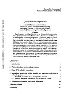
Figure (2) shows superpositions of OAM modes in two different bases: the LG basis and the Bessel-Gauss (BG) basis.
5
Figure 2: Intensity distributions for superposition modes of OAM for different azimuthal indices. For each image, the superposition is between and . Both bases, LG and BG, can be used to measure OAM. The higher order Bessel modes vary with the azimuthal phase index23.
Entangled states in OAM The seminal paper by Mair et al.8 was the first experiment to demonstrate OAM as a property of single photons produced by SPDC. They showed that OAM is conserved in the SPDC process and consequently showed entanglement involving these modes24. That is, the OAM of the entangled photon pair must sum to the OAM of the pump. The two-photon state for OAM can be written as , where
is the probability of finding one photon in state
, where the pump beam has zero OAM. As
6
(9) and the other in state
can assume any integer value, Eq.
(9) is true for d–dimensional two-photon states, where
ranges over d different
values. The conjugate variable of OAM is angular position, which can be described by an aperture with an angular width
. Similar to Heisenberg’s uncertainty relationship
between momentum and position, the relationship between OAM and angular position is described by25, .
(10)
A violation of the inequality in Eq. (10) satisfies the EPR-Reid criterion26, which is analogous to the original EPR paradox. These correlations demonstrate entanglement not only for discrete variables such as OAM but for continuous variables like angular position as well.
Generation of entangled photons The most commonly used and most efficient method of producing entangled photon pairs is that of spontaneous parametric down conversion (SPDC)27. This non-linear optical process decays a pump photon into two photons (signal and idler) in a crystal of optical non-linearity,
. Both energy and momentum are conserved in this decay
process, also known as the phase matching conditions: (11) (12) Here,
are the frequencies and
the wave vectors of the pump,
signal and idler photon, respectively.
Figure 3: Phase matching conditions for non-collinear and collinear SPDC.
Due to these conditions, the measurement of one photon in a particular direction and energy, forces the existence of the other correlated photon pair of definite energy and direction. There are two types of SPDC, namely type I and type II. In type I, the
7
down-converted photons are produced with the same polarisation, orthogonal to that of the pump. Photons of the same wavelength are emitted on concentric cones centred around the pump axis of propagation. The diameter of the cone depends on the angle between the pump beam and the optical axis of the crystal. Type II SPDC emits one photon with the same polarisation as the pump and the other with orthogonal polarisation. In both cases, the process is said to be degenerate if the down-converted photon pair have the same wavelength (i.e.
) and non-degenerate
otherwise. SPDC can be further characterised into collinear and non-collinear processes, depending on the position of the optic axis relative to the pump. By simply changing the tilt of the crystal, we are able to change the opening angle of SPDC, moving from non-collinear to collinear down-conversion [see Fig. (4)], allowing an optimal position to be found depending on the application.
Figure 4: SPDC is the most efficient method for producing entangled photons, however, the probability of a spontaneous decay into a pair of entangled photons is very low, approximately 1 in every photons are down-converted. Therefore a very sensitive electron multiplier CCD camera is needed to image the ring of photons. (a) Far-field image of the collinear down-converted light from the BBO crystal. (b) Far-field image of the nearcollinear down-converted light from the BBO crystal. (c) Far-field image of the non-collinear down-converted light from the BBO crystal. The change from non-collinear to collinear requires a very small change in tilt.
It has been found that the intensity profile of the far-field down-converted light follows the function28 , where
(13)
is the focal length of the Fourier lens with radial coordinate
. The phase-
matching parameter establishes the opening angle of SPDC and is given by , and
, for refractive index
, crystal
length L. The propagation of light through an optical system can be described by étendue, which when normalised to the wavelength
8
, gives an estimate of the
number of detectable transverse modes, written as29 .
(14)
Here, A is the area of the near-field beam and
is the far-field opening angle. We
have chosen to measure OAM entanglement in the near-field, effectively setting A to be constant. Thus, as we change
from collinear to near-collinear, the opening angle
increases, yielding a larger OAM spectrum.
Spiral bandwidth We know that SPDC produces pairs of photons that are entangled in OAM8. The number of OAM modes generated in this process is known as the generation spiral bandwidth and is dependent on two main factors: the size of the pump beam and the length of the crystal. As the radial intensity distribution increases with
, the size of
the pump waist determines the highest OAM mode achievable. Thus a larger pump waist is favourable over a tightly focused spot. The phase matching conditions become more restrictive for thicker crystals, which consequently diminishes the probability of generating higher OAM modes. A thinner crystal (e.g. 0.5 mm thick) will produce a wider spectrum of OAM modes, but at the cost of efficiency. A compromise between the spiral bandwidth and efficiency will be determined by the aim of the experiment. The bandwidth generated at the crystal is not necessarily the bandwidth detected. This is dependent on the design of the experiment, including the single-photon source, the measurement methods and the detection components. The following section describes each aspect of the experimental setup used to demonstrate quantum entanglement.
Experimental design Components Figure 5 shows a general idea of the design of the experiment. A source to generate single photon pairs is an obvious requirement. As previously mentioned, SPDC is a widely used method, which we too use for this paper. A particular property of a photon needs to be chosen so as to determine the measurement scheme. Such properties include the measurement of the conjugate variables energy and time, or momentum and position. We chose to measure the OAM of photons mainly owing to
9
its potential for high dimensional entanglement and the ease at which we can measure OAM using SLMs. Finally, we also need a method to detect not only single photons but also the coincidence counts from entangled photon pairs.
Figure 5: Schematic of the experimental setup used to generate, measure and detect entangled photons. The source, S, generates the photon pairs, which are then measured in a particular basis at M and then finally detected at D.
We examine these experimental segments to highlight the challenges involved in setting up each. Source The SPDC process requires a balance between generating sufficient photon pairs for reasonable counting times, and errors introduced when many photon pairs are produced within the same time window. The balance between these parameters is largely determined by the energy and the repetition rate of the pump source. In our experiment a mode-locked ultraviolet pump source with a wavelength of 355 nm and average power of 350 mW was used. The laser produces pulses at 80 MHz, each pulse made up of ~109 photons. The SPDC process produces on average 1 photon pair in every ~105 pulses, or 800 per second. This relates to an efficiency of ~10-12. The time between photon pairs in turn dictates the time window of the detection system (gating time). Since the pulses arrive at intervals of 12.5 nanoseconds, we select a gating time of 12.5 nanoseconds to minimise the error of multiple photon pairs arriving at the same time. The high repetition rate of the laser is only possible with mode-locked systems, and is used here only as a means to increase the sample rate. Increasing the energy of the pulse would also increase the pair production rate through an improved efficiency of the SPDC process.
Unfortunately this also
increases the error in the system by way of multiple pair generation. The length of the non-linear crystal also has an effect on the SPDC efficiency, that is, a thicker crystal will produce more photon pairs per pulse. We observed an increase in coincidence counts when changing from a 0.5-mm-thick crystal to a 3-mm-think crystal of approximately three times. However, this must be weighed up against the generated spiral bandwidth (the width of the distribution of OAM modes), which is also
10
dependent upon crystal length. Measurement A spatial light modulator enables the phase of an incoming beam to be shaped according to the encoded hologram. That is, a Gaussian beam illuminating a phaseonly forked hologram of particular azimuthal index,
, produces a helically-phased
beam in the first diffraction order. This process also operates in reverse, in that a beam with OAM
incident on a forked hologram with an azimuthal index
, will
produce a Gaussian beam.
Figure 6: A spatial light modulator encoded with an azimuthal phase dependence,
,
shapes a Gaussian beam into a helically-phased beam in the first diffraction order. This process also works in reverse such that an LG beam can be converted into a Gaussian beam.
Only the fundamental mode (a Gaussian beam) can propagate through single-mode fibres (SMF). The hologram on the SLM together with the SMF, act as a “matchfilter” such that an incoming beam with OAM
will only couple into the SMF if the
hologram is encoded with the same azimuthal phase index, . The angular position states are measured by defining a narrow “slice” of the hologram30, representing an aperture [see Fig. (7)]. The orientation and width of the aperture can be varied; however, a very narrow slice results in a significant reduction in the number of coincidence counts detected. Thus, there is a minimum limit to which the width can be defined.
11
Figure 7: Hologram used to measure angular position correlations. The conjugate variable of OAM is angular position. By setting a particular aperture, we can measure the angular position correlations by varying the aperture width and its orientation.
Detection The detection of photon pairs requires particular devices, which are both electronically fast and efficient. The single photons are typically measured using avalanche photo-diodes (APDs) with a quantum efficiency of approximately 60%. Evidently, the laboratory must be as dark as possible when using single photon detectors. Nonetheless, the measured dark count rate, the single photon count rate of the dark laboratory without lasing source, is approximately
as the laboratory
does allow in some external light. The coincidence count rate is recorded using a coincidence counter connected to two single photon detectors. When a photon is detected by one detector it starts the trigger in the second detector and when a photon arrives in the second, a coincidence is recorded. Of course, there must be a limit placed on the interval in which the second photon is detected, known as the gating time. There are a number of counting instruments available, which vary in price and gating time. The HydraHarp 400 was used with a gating time set at 12.5 ns. Even with a very narrow time interval, uncorrelated photon coincidence counts may be recorded, know as accidental counts and can be estimated as from each detector and
, where is the gating time.
12
and
are the single count rates
Experiment
Figure 8: Experimental setup used to detect the OAM eigenstate after SPDC. The plane of the crystal was relay imaged onto two separate SLMs using lenses, L1 and L2 (f1 = 200 mm and f2 = 400 mm), where the LG modes were selected. Lenses L3 and L4 (f3 = 500 mm and f4 = 2 mm) were used to relay image the SLM planes through 10 nm band-width interference filters (IF) to the inputs of the single-mode fibres (SMF).
Figure 8 shows our experimental setup. A mode-locked ultraviolet pump source with a wavelength of 355 nm and average power of 350 mW was used to pump a 3-mmthick type I barium borate (BBO) crystal to produce collinear, degenerate entangled photon pairs via SPDC. An interference filter was placed after the crystal to reflect the pump beam and transmit the 710 nm down-converted light. The front plane of the crystal was then imaged (f1 = 200 mm, f2 = 400 mm) onto two separate phase-only spatial light modulators (SLMs). Just as polarisers were used to “select” a particular polarization state, the SLMs allow a specific state to be chosen into which the photon will be projected. Initially, the Laguerre-Gaussian basis set was chosen to measure the OAM states, however any orthogonal basis set can be chosen such as the BesselGaussian basis23. The SLM planes were then reimaged (f3 = 500 mm, f4 = 2 mm) and coupled into single-mode fibres (mode-field diameter =
) so as to extract only
the Gaussian modal components. Interference filters centred at 710 nm were placed in front of each fibre coupler to prevent any scattered pump light to enter the fibres. The fibres connected to single-photon avalanche detectors allowed the arrival of a photon pair to be registered using a HydraHarp 400 coincidence counter.
13
Table 1: Specifications of the experimental equipment used to perform quantum entanglement.
Equipment
Manufacturer
Specifications
Laser source
Newport
355 nm, 350 mW
Non-linear crystal
Castech
BBO, type I, degenerate
Spatial light modulator
HoloEye
Phase-only, NIR, 1920x1080 pixels
Interference filters
Thorlabs
Central wavelength: 710 +/- 10 nm
Single-mode fibre
Thorlabs
630-680 nm
Avalanche photodiodes
Perkin Elmer
Dark count ~ 200 counts
Coincidence counter
PicoQuant: HydraHarp400
8 channels
An object can be imaged in two ways, either using a single lens (2f-imaging system) between the object and image plane or using two lenses (4f-imanging system). While both methods image the intensity of the object, only the latter method images both the intensity and phase of the object. This is important when considering the properties of two-photon correlations31, as the wave fronts of the signal and idler beams must sum to that of the pump beam in order to detect a coincidence signal. An additional lens function can be added to the SLM to compensate for a mismatch in wave fronts. However this method requires additional optimisation for each SLM. A simpler and more effective method, which we use in our experimental setup, makes use of a 4fimaging system. Assuming the pump beam has a planar wave front at the crystal, a 4fimaging scheme will image modes with planar wave fronts onto both SLMs. As the down-conversion process is not very efficient, alignment of the system becomes rather difficult. We used a method of “back projection” or “retrodiction”, first proposed by Klyshko32, to align the system, by passing a 710 nm diode laser beam through each of the single mode fibres so as to pass through the system in reverse. There are a number of benefits in using this method. Firstly, the pump beam and both back-projected beams must overlap at the plane of the crystal. Initially the SLMs were switched off and therefore only acted as mirrors, allowing a single beam to be aligned with the pump beam. Thereafter, the SLMs were switched on with a grating hologram to separate the diffraction orders. The tilt of the
14
SLMs was changed such that the first diffraction order from each SLM was overlapped with the pump beam. The measured coincidences can also be numerically determined by calculating the overlap integral of the back-projected signal, idler beams with the pump field at the crystal plane. The coincidence rate is proportional to the overlap intergal33, that is, ,
where
,
and
are the modes of the signal, idler and pump beams,
respectively. If a back-projected beam of the overlap for
is of equal size with the pump, then
will be very strong, while higher OAM modes, whose intensity
distribution increases with projected beam of the
(15)
, will have very weak overlaps. Thus, if the back-
is smaller than the pump, the overlap will be less strong for
mode but also more significant in higher modes. The ratio of the pump waist is given as34:
with the signal (idler) waist
.
(16)
In terms of the imaging systems shown in Fig. (8), we calculated our ratio to be . This appears to be a fair ratio when finding a balance between efficiency and spiral bandwidth. Miatto et al.34 investigate three different ratios; 0.5, 2 and 4 with regard to LG modes with increase with
. They show that although the spiral bandwidth does
, the count rate for
drops almost to the accidental count rate.
Back-projection also allows us to view the modes that we generate on the SLMs, which guarantees that we are indeed measuring in the correct basis. We placed a flipup mirror between the BBO crystal and lens L1 so as to reflect the back-projected light onto a CCD camera (placed 200 mm from L1). The alignment of the beam with the centre of the hologram is very important, as seen in Fig. (9), where a misaligned beam results in an uneven intensity distribution.
15
Figure 9: The alignment of the beam with the centre of the SLM has a significant effect on the coincidence measurements, such that measurements with a theoretically value of zero become non-zero with misalignment.
On the single photon level, this uneven distribution corresponds to measuring nonzero coincidence counts where there should be none. Back-projection provides visual confirmation that the beam is centred on the hologram. However, we performed an additional optimisation on the spatial position of the beam on the SLM using the knowledge that OAM is conserved in down-conversion. That is, for a pump beam with OAM of
, we would only expect to see a coincidence count when
. Thus, if a hologram of
is encoded onto SLM A and
on SLM
B, we do not expect to observe any coincidence counts. If we do see counts, the hologram is repositioned until a minimum count rate is obtained and then repeated for on SLM A. The measurements of OAM are sensitive to lateral position alignment, while the angular position measurements are sensitive to the axial positions of the image planes. Observing the back-projected beam on the CCD allowed us to ensure both SLMs were placed in the correct image plane. Both lenses L1 and L2 were placed upon micrometer translation stages to allow for small adjustments along the axis of propagation to find the correct image plane. The size of variable aperture between lenses L1 and L2 was decreased until a clear image of the “slice” was seen. Once each step was carefully executed, both single-mode fibres were connected to their respective detectors and the flip-up mirror was moved out of the beam path. With the UV laser pumping the crystal, the coincidence count rate was recorded. A few minor adjustments were made to the angular position of both SLMs so as to
16
maximise the coincidence count rate.
Quantum measurements After following a rigorous alignment procedure, we were able to perform a number of fundamental tests. The first of which was to demonstrate the conservation of OAM. Each SLM was encoded with holograms ranging
from -20 to 20, one after another.
Figure 10 shows the measured coincidence counts known commonly as the spiral bandwidth.
Figure 10: Experimental results showing (a) a density plot of the coincidence counts per second and (b) the non-zero diagonal elements representing a spiral bandwidth plot. The FWHM of the spiral bandwidth is approximately 15.
The anti-correlated diagonal is consistent with OAM conservation, that is
.
While the coefficients in the OAM spectrum demonstrate a decreasing trend from , the size of the mode is another contributing factor as the mode increases with the azimuthal index, which results in a loss of efficiency, resulting in a decreasing trend from
. Another important feature obtained from Fig. (10a) is the values of
the off diagonal elements. Theoretically these should be zero, but experimentally this is often impossible to achieve as the spiral bandwidth is highly sensitive to misalignment. We measured the off-diagonal elements to be less than 5% of their corresponding diagonal element. From Fig. (10b) we measured the full-width-halfmaximum (FWHM) value to be 15. The spiral bandwidth experiment offers an effective method to test whether the setup is correctly aligned. Similarly, the angular position can be used to ensure the optics are placed in the correct image planes. An angular sector hologram was encoded onto
17
each SLM; one hologram fixed at a particular orientation while the other hologram rotated in small increments through
. In a ghost imaging experiment, an aperture is
placed in one arm and the detector in the other arm is scanned through its transverse position, resulting in the reconstruction of the aperture shape. Similarly, the width of the angular hologram was determined from the measured coincidence counts. A sharp coincidence peak was recorded when the holograms were both orientated at the same angle, see Fig. (11), where the width of the peak gives the width of the angular “slice”.
Figure 11: Experimental measurements showing (a) a density plot of the coincidence counts per second using the angular holograms. The holograms on each SLM were rotated through
. (b) Probability distribution of the angular position
for
, taken along
the red dotted line in (a).
From the data recorded for both the spiral and angular bandwidths, we calculated the uncertainty relationship between the two. A profile from the centre of each spectrum was plotted and fitted with a Gaussian distribution (Fig. (12)), which gave the following widths
and
taking the product of the two
. Therefore, by , the EPR-Reid criterion is
violated as the product is clearly smaller than the uncertainty relation of 0.25 in Eq. (10).
18
Figure 12: Probability distributions for (a) the OAM position
for
for
and (b) the angular
. A Gaussian distribution has been fitted to both to determine the
widths of each plot, which were used to demonstrate the EPR-Reid criterion.
Bell inequalities The EPR paradox does not eliminate the possibility of hidden variables. To do this, a violation of Bell’s inequality must be shown. In order to demonstrate this, the correlations between the two entangled photons must also be observed for superposition states35, described by . Here
(17)
denotes the degree of rotation. By choosing a particular value for , we
generated superposition holograms for a range of angles . The holograms were varied on both SLMs, by fixing one at orientation
and rotating the other
, and
the coincidence count rates were measured. Bell showed that the sinusoidal behaviour seen in figure B cannot be simulated by classical correlations and the deviation from classical theory can be calculated using Bell’s inequality or a variation thereof derived by Clauser et al2.
19
Figure 13: The normalised coincidence counts as a function of the orientation of the holograms on each SLM. The orientation of the hologram on SLM A was fixed while those on SLM B were rotated from 0 to
.
The Bell parameter S can be defined as35: . Where
is a different orientation from
measured coincidence counts
.
(18)
is calculated directly from the
at particular orientations,
. (19)
The inequality is violated when an entangled system is
. For the CHSH inequality, the upper limit for . For
inequality by 26 standard deviations,
, we observed a violation of the , indicating an entangled system.
State tomography Lastly, it is important to form a characterisation of the entangled states by measuring the degree of entanglement. This is attained by performing a state tomography on the system. We previously introduced the concept of a density matrix used to describe the statistical state of a quantum system. Using particular coincidence measurements, we are able to reconstruct36 the two-photon density matrix: (20)
20
where
focused on the equator states states
. From the Bloch sphere22, we
represents the Pauli matrices for
and
in Eq. (16) together with the pure
, shown in Fig. (14).
Figure 14: Holograms used to perform a state tomography on the system with the aim of calculating the density matrix. These include two pure states and the corresponding four superposition states. All six holograms were cycled through on each SLM, resulting in 36 coincidence measurements.
In matrix form, the qubit density matrix is written as:
(21)
Here
and
are the amplitudes and phases of the density matrix elements. The
probability to detect one photon in state
and the other in state
is expressed by
the diagonal terms. The off-diagonal terms are determined from measurements in the superposition states. We generated six different states on each SLM, resulting in a total of 36 coincidence measurements. Therefore for a two-dimensional state, we use an over-complete set of measurements (36) to determine the 16 density matrix elements. We used a least squares fitting program to calculate the best density matrix according to our measurements. We followed the procedure in Jack et al.36 where the 10 amplitudes and 6 phases from the density matrix in Eq. (21) are chosen such that the following equation is minimised: (22)
21
The experimentally measured coincidence counts are represented by counts predicted from the density matrix are given by
and the
. In matrix form, the two-
dimensional reconstructed density matrix was calculated to be
.
(23)
Eq. (23) shows the real and imaginary parts of the density matrix, shown graphically in Fig. (15).
Figure 15: Graphically representation of the (a) real and (b) imaginary parts of the twodimensional density matrix.
As previously mentioned, the density matrix can be used to calculate various quantifying parameters. Firstly, the linear entropy37
defines the
purity of the system, where the linear entropy of a pure entangled state is zero. We calculate a linear entropy of 0.02 for the above density matrix. The fidelity is a measure of how close our reconstructed state is to the target state, which is the (pure) maximally entangled state in this case. The fidelity is given by . Here,
is the target state with
is our measured reconstructed state. We measured a fidelity of indicating that our reconstructed state can be considered a pure ( entangled state.
22
(24) and , ), maximally
We chose to study OAM entanglement with the objective of measuring entanglement in higher dimensions. The above mentioned density matrix was reconstructed using two bits of information per photon, that is
and its superpositions. However, in
high-dimensional entanglement we encode multiple bits of information per photon. For example, for dimension dimension
, we could use
, we could use
or
and for
. An equivalent density matrix to Eq.
(20) can be written for d-dimensions as, , where
are complex coefficients with
Mann matrices39 are represented by
(25) for normalisation. The Gell-
for
and
identity matrix. Thus, following a similar procedure used for the density matrix for higher dimensions from
to
is the d-dimensional , we reconstructed
. A detailed description
on similar measurements can be found in Agnew et al.40 The linear entropy and fidelity of each density matrix was calculated and plotted in Fig. (16).
Fig. 16: (a) Fidelity and (b) linear entropy as a function of dimension. The red triangles represent the experimental measurements, while the blue dots represent the threshold states in Eq. (26).
23
The results indicate that the degree of entanglement decreases as the dimensionality increases, however the results do not fall below the threshold states, which lie on the threshold of the high-dimensional Bell inequality41. These are given by , where
is the probability above which the Bell inequality is violated,
(26) is the
maximally entangled state of two d-dimensional systems and I is the identity matrix of dimension
.
Discussion We have demonstrated a method to achieve a quantum entanglement setup together with procedures to measure and quantify the entangled system. By using the OAM basis we can choose to perform measurements in two-dimensional entangled states, or extend the setup to higher dimensions by altering the phase holograms used in the measurement scheme40. For example, we have shown a violation of a Bell-type inequality for dimension two and high fidelity states in dimension five (Hilbert space of dimension twenty five). High-dimensional entanglement offers further possibilities such as closing the detection loophole in Bell experiments42. Likewise, instead of using a Gaussian shaped source to pump the crystal, any number of pump shapes can be used, for example a Hermite-Gaussian beam43. In so doing, the down-conversion process can be better understood, possibly improving the measured spiral bandwidth.
References 1. Einstein A, Podolsky B, Rosen N. Can quantum-mechanical description of physical reality be considered complete? Phys. Rev. 1935; 47: 777-780. 2. Clauser J, Horne M, Shimony A, Holt R. Proposed experiment to test local hidden-variable theories. Phys. Rev. Lett. 1969; 23: 880–884. 3. Freedman S, Clauser J. Experimental test of local hidden-variable theories. Phys. Rev. Lett. 1972; 28: 938–941. 4. Clauser J. Experimental investigation of a polarization correlation anomaly. Phys. Rev. Lett. 1976; 36: 1223–1226. 5. Aspect A, Grangier P, Roger G. Experimental tests of realistic local theories via bell’s theorem. Phys. Rev. Lett. 1981; 47: 460–463.
24
6. Aspect A, Grangier P, Roger G. Experimental realization of einsteinpodolskyrosen-bohm gedankenexperiment: A new violation of bell’s inequalities. Phys. Rev. Lett. 1982; 49: 91–94. 7. Shih Y, Alley C. New type of einstein-podolsky-rosen-bohm experiment using pairs of light quanta produced by optical parametric down conversion. Phys. Rev. Lett. 1988; 61: 2921–2924. 8. Mair A, Vaziri A, Weihs G, Zeilinger A. Entanglement of the orbital angular momentum states of photons. Nature 2001; 412: 313–316. 9. Bennett C, Di Vincenzo D. Quantum information and computation. Nature. 2000; 404: 247–255. 10. Jennewein T, Simon C, Weihs G, Weinfurter H, Zeilinger A. Quantum crytography with entangled photons. Phys. Rev. Lett. 2000; 84: 4729–4732. 11. Bouwmeester D, Pan J, Mattle K, Eibl M, Weinfurter H, Zeilinger A. Experimental quantum teleportation. Nature. 1997; 390: 575–579. 12. Nielsen MA, Chuang IL. Quantum computation and quantum information. Cambridge: Cambridge University Press; 2009. 13. Gisin N, Ribordy G, Tittel W, Zbinden H. Quantum cryptography. Rev. Mod. Phys. 2002; 74:145-195. 14. Kwiat PG, Steinberg AM, Chiao RY. High-visibility interference in a Bellinequality experiment for energy and time. Phys. Rev. A. 1993; 47: R2472R2475. 15. Rarity JG, Tapster PR. Experimental violation of Bells inequality based on phase and momentum. Phys. Rev. Lett. 1990; 64: 2495 – 2498. 16. Howell JC, Bennink RS, Bentley SJ, Boyd RW. Realization of the EinsteinPodolsky-Rosen Paradox UsingMomentum- and Position-Entangled Photons from Spontaneous Parametric Down Conversion. Phys. Rev. Lett. 2004; 92: 210403. 17. Shih Y. Entangled biphoton source – property and preparation. Rep. Prog. Phys. 2003; 66: 1009 – 1044. 18. Rangarajan R, Goggin M, Kwiat P. Optimizing type-I polarization-entangled photons. 2009; 17: 18920 – 18933. 19. Allen L, Beijersbergen M, Spreeuw R, Woerdman J. Orbital angular momentum of light and the transformation of Laguerre-Gaussian laser modes. Phys. Rev. A. 1992; 45: 8185–8189.
25
20. Volke-Sepulveda K, Garcés-Chávez V, Chávez-Cerda S, Arlt J, Dholakia K. Orbital angular momentum of a high-order Bessel light beam. J. Opt. B: Quantum Semiclass. Opt. 2002; 4: S82 – S89. 21. Bandres MA, Gutiérrez-Vega JC. Ince gaussian beams. Optics Lett. 2004; 29(2): 144-146. 22. Padgett MJ, Courtial J. Poincare-sphere equivalent for light beams containing orbital angular momentum. Opt. Lett. 1999; 24: 430–432. 23. McLaren M, Agnew M, Leach J, et al. Entangled Bessel-Gaussian beams. Opt. Express. 2012; 20: 23589-23597. 24. Vaziri A, Weihs G, Zeilinger A. Experimental two-photon, three dimensional entanglement for quantum communication. Phys. Rev. Lett. 2002; 89: 240401. 25. Franke-Arnold S, Barnett SM, Yao E, Leach J, Courtial J, Padgett MJ. Uncertainty principle for angular position and angular momentum. New J. of Phys. 2004; 6 (103): [8]. 26. Reid MD. Demonstration of the Einstein-Podolsky-Rosen paradox using nondegenerate parametric amplification. Phys. Rev. A. 1989; 40: 913 – 923. 27. Ou ZY, Mandel L. Violation of bell's inequality and classical probability in a two-photon correlation experiment. Phys. Rev. Lett. 1988; 61: 50–53. 28. Romero J, Giovannini D, Franke-Arnold S, Barnett SM, Padgett MJ. Increasing the dimension in high-dimensional two-photon orbital angular momentum entanglement. Phys. Rev. A. 2012; 86: 012334(6). 29. van Exter MP, Aiello A, Oemrawsingh SSR, Nienhuis G, Woerdman JP. Effect of spatial filtering on the Schmidt decomposition of entangled photons. Phys. Rev. A. 2006; 74: 012309(4). 30. Leach J, Jack B, Romero J, et al. Quantum correlations in optical angle-orbital angular momentum variables. J. of Opt. 2010; 329: 662 – 665. 31. Pittman TB, Strekalov DV, Klyshko DN, Rubin MH, Sergienko AV, Shih YH. Two-photon geometric optics. Phys. Rev. A. 1996; 53: 2804 – 2815. 32. Klyshko D. A simple method of preparing pure states of an optical field, of implementing the Einstein–Podolsky–Rosen experiment, and of demonstrating the complementarity principle. Soviet Physics Uspekhi. 1988; 31: 74 – 85. 33. Franke-Arnold S, Barnett SM, Padgett MJ, Allen L. Two-photon entanglement of orbital angular momentum states. Phys. Rev. A. 2002; 65: 033823(5). 34. Miatto F, Giovannini D, Romero J, Franke-Arnold S, Barnett SM, Padgett MJ.
26
Bounds and optimisation of orbital angular momentum bandwidths within parametric down-conversion systems. Eur. Phys. J. D. 2012; 66: 178. 35. Leach J, Jack B, Romero J, et al. Violation of a bell inequality in twodimensional orbital angular momentum state-spaces. Optics Express. 2002; 17: 8287–8293. 36. Jack B, Leach J, Ritsch H, Barnett S, Padgett MJ. Precise quantum tomography of photon pairs with entangled orbital angular momentum. New J. of Phys. 2009; 811: 103024. 37. White AG, James DFV, Munro WJ, Kwiat PG. Exploring Hilbert space: Accurate characterization of quantum information. Phys. Rev. A. 2001; 65: 012301. 38. Wootters WK. Entanglement of formation of an arbitrary state of two qubits. Phys. Rev. Lett. 1998; 80: 2245–2248. 39. Peskin ME, Schroeder DV. An introduction to quantum field theory. Don Mills, Canada: Addison-Wiley Publishing Company; 1995. 40. Agnew M, Leach J, McLaren M, Roux FS, Boyd RW. Tomography of the quantum state of photons entangled in higher dimensions. Phys. Rev. A. 2011; 84: 062101. 41. Collins D, Gisin N, Linden N, Massar S, Popescu S. Bell inequalities for arbitrarily high-dimensional systems. Phys. Rev. Lett. 2002; 88: 040404. 42. Vertesi T, Pironio S, Brunner N. Closing the detection loophole in Bell experiments using qudits. Phys. Rev. Lett. 2010; 104: 060401. 43. Romero J, Giovannini D, McLaren MG, Galvez EJ, Forbes A, Padgett MJ. Orbital angular momentum correlations with a phase-flipped Gaussian mode pump beam. J. Of Optics. 2012; 14: 085401.
27