Realm-Based Spatial Data Types: The ROSE Algebra1
Ralf Hartmut Güting Markus Schneider Praktische Informatik IV, FernUniversität Hagen Postfach 940, D-5800 Hagen, Germany
[email protected],
[email protected]
Abstract: Spatial data types or algebras for database systems should (i) be fully general (which means, closed under set operations, hence e.g. a region value can be a set of polygons with holes), (ii) have formally defined semantics, (iii) be defined in terms of finite representations available in computers, (iv) offer facilities to enforce geometric consistency of related spatial objects, and (v) be independent of a particular DBMS data model, but cooperate with any. We offer such a definition. A central idea is to use realms as geometric domains underlying spatial data types. A realm as a general database concept is a finite, dynamic, user-defined structure underlying one or more system data types. A geometric realm defined here is a planar graph over a finite resolution grid. Problems of numerical robustness and topological correctness are solved below and within the realm layer so that spatial algebras defined above a realm enjoy very nice algebraic properties. Realms also interact with a DBMS to enforce geometric consistency on object creation or update. The ROSE algebra is defined on top of realms and offers general types to represent point, line, and region features together with a comprehensive set of operations. It is described within a polymorphic type system and interacts with a DBMS data model and query language through an abstract object model interface. An example integration of ROSE into the object-oriented data model O2 and its query language is presented.
Keywords: Spatial data types, algebra, realm, finite resolution, numerical robustness, topological correctness, geometric consistency, object model interface, ROSE.
1
This work was supported by the DFG (Deutsche Forschungsgemeinschaft) under grant Gu 293/1-1
−
1
−
1 Introduction We consider a spatial database system to be a full-fledged DBMS with additional capabilities for the representation and manipulation of geometric data. As such, it provides the database technology needed to support applications such as geographic information systems. The standard DBMS view for the organization of spatial information is the following: A database consists of several classes of objects. A spatial object is just an object with an associated value (“attribute”) of a spatial data type, such as, for example, point, line, or region. This is true regardless of whether the DBMS uses a relational, complex object, object-oriented or some other data model. Hence the definition and implementation of spatial data types is probably the most fundamental issue in the development of spatial database systems. Although spatial data types (SDTs) are used routinely in the description of spatial query languages (e.g. [LiN87, JoC88, SvH91, To90]), have been implemented in some prototype systems (e.g. [RoFS88, OrM88, Gü89]), and some formal definitions have been given [Gü88a, ScV89, GaNT91], there is still no completely satisfactory solution available according to the following criteria: • Generality. The geometric objects used as SDT values should be as general as possible. For example, a region value should be able to represent a collection of disjoint areas each of which may have holes. More precisely, this means that the domains of data types point, line, and region must be closed under union, intersection, and difference of their underlying point sets. This allows for the definition of powerful data type operations with nice closure properties. • Rigorous definition. The semantics of SDTs, that is, the possible values for the types and the functions associated with the operations, must be defined formally to avoid ambiguities for the user and the implementor. • Finite resolution. The formal definitions must take into account the finite representations available in computers. This has so far been neglected in definitions of SDTs. It is left to the programmer to close this gap between theory and practice which leads rather inevitably not only to numerical but also topological errors. • Treatment of geometric consistency. Distinct spatial objects may be related through geometric consistency constraints (e.g. adjacent regions have a common boundary). The definition of SDTs must offer facilities to enforce such consistency. • General object model interface. Spatial data types as such are rather useless; they need to be integrated into a DBMS data model and query language. However, a definition of SDTs should be valid regardless of a particular DBMS data model and therefore not depend on it.2 Instead, the SDT definition should be based on an abstract interface to the DBMS data model which we call the object model interface. The purpose of this paper (together with a companion paper [GüS93]) is to develop a formal definition of spatial data types fulfilling these criteria. A central idea is to introduce into the DBMS the concept of a realm. A realm is in general a finite, user defined structure that is used as a basis for one or more system data types. Realms are somewhat similar to enumeration types in programming languages. A realm used as a basis for spatial data types is essentially a finite set of points and non-intersecting line 2
This also holds for the implementation level: A spatial type extension package (STEP) should be able to cooperate with any extensible DBMS offering a suitable interface regardless of its data model.
−
2
−
segments. Intuitively, it describes the complete underlying geometry of an application. All points, lines and regions associated with objects (from now on called spatial attribute values) can be defined in terms of points and line segments present in the realm. In fact, in a database spatial attribute values are then never created directly but only by selecting some realm objects. They are never updated directly. Instead, updates are performed on the realm and from there propagated to the dependent attribute values. Hence, all attribute values occurring in a database are realm-based. Furthermore, the algebraic operations for the spatial data types are defined to construct only geometric objects that are realmbased as well. So the spatial algebra is closed with respect to a given realm. This means in particular that no two values of spatial data types occurring in geometric computation have “proper” intersections of line segments. Instead, two initially intersecting segments have already been split at the intersection point when they were entered into the realm. One could say that any two intersecting SDT values (say, lines or regions) “have become acquainted” already when they were entered into the realm. This is a crucial property for the correct and efficient implementation of geometric operations. Realm objects - points and segments - are defined not in abstract Euclidean space but in terms of finite representations. All geometric primitives and realm operations (e.g. updates) are defined in error-free integer arithmetic. For mapping an application’s set of intersecting line segments into a realm’s set of non-intersecting segments the concept of redrawing and finite resolution geometry from [GrY86] is used. Although intersection points computed with finite resolution in general move away from their exact Euclidean position, this concept ensures that the unavoidable distortion of geometry (that is, the numerical error) remains bounded and very small and that essentially3 no topological errors occur. This means that a programmer has a precise specification that directly lends itself to a correct implementation. It also means that the spatial algebra obeys algebraic laws precisely in theory as well as in practice. Furthermore, it is rather obvious that realms also solve the geometric consistency problem. Most closely related to this work are the formal definitions of spatial data types (or algebras) given by Güting [Gü88a, Gü88b], Scholl and Voisard [ScV89, Vo92], and Gargano et al. [GaNT91]. All of these proposals do not fulfill most of the criteria given above. In [Gü88a, Gü88b] data types for points, lines, and regions are available but too restricted, e.g. a region is a single simple polygon (without holes). In [ScV89] general regions are defined; in Voisard’s thesis [Vo92] this has been extended to general types for points and lines. However, the definitions are unnecessarily complex. In [GaNT91] there is only a single type for all kinds of geometric objects; a value is essentially a set of sets of pixels. We feel this is not sufficient, since many interesting spatial operations cannot be expressed. As mentioned, all of these proposals give formal definitions. However, those of Güting and of Scholl and Voisard are not based on finite resolution; hence the numeric correctness problems are not addressed. Gargano et al. base their definitions in principle on a finite underlying set (of pixels). But this is not practical since these finite representations are far too large to be efficiently manageable. The geometric consistency problem is not solved in any of these proposals; there is some weak support in [Gü88a] through an area data type, but it is not sufficient. Finally, all three proposals have connected their spatial types to a fixed data model − Güting and Gargano et al. to the relational model and Scholl and Voisard to a complex object algebra. Only Scholl and Voisard emphasize a clean interface 3
See the discussion in Section 2 and in [GüS93].
−
3
−
between the spatial algebra and the general object model. We shall extend their work by offering an abstract interface not dependent on any particular data model. Separating geometric primitives from the remainder of geometric modeling was already proposed by Frank and Kuhn [FrK86]. Because of the conflict between the infinite precision real numbers of Euclidean geometry and the finite precision number systems of computers they suggest to abandon coordinate-based geometry and to only consider the topological structures of point sets underlying spatial values. Their topological data model (later continued in [EgFJ89]) is based on simplicial complexes and has a similar purpose as our concept of realms. Essentially they offer an irregular triangular network partition of the plane as a geometric domain over which spatial objects could be defined. However, the connections are missing to the underlying finite arithmetic as well as to spatial data types based on this model. Also, in our view a triangular partition contains too much information; it is sufficient to keep those points and segments in a geometric domain that are needed for spatial attribute values. Finally, their model is an abstract one whereas we show realms within a database context. Our description and formal development of realm-based spatial data types is given in two papers. In the first paper [GüS93] the lower layers, namely numerically robust geometric primitives, realms and their update operations and a number of realm-based structures (cycles, faces, ...) and primitives have been defined. In this paper spatial data types points, lines, and regions and their operations, that is, the spatial algebra (called ROSE algebra), are described and defined formally. Related issues such as modeling partitions of the plane within the type system and an abstract object model interface are addressed. We also show how the ROSE algebra can be integrated with a DBMS data model and query language, using O2 as an example. In the following section we first provide an informal overview of the complete concept.
2 Overview: Realm-Based Spatial Data Types A realm is a set of points and non-intersecting line segments over a discrete domain, that is, a grid, as shown in Figure 1.
Figure 1: Example of a realm Values of spatial data types can be composed from the objects present in a realm. Figure 2 shows some values definable over the realm of Figure 1. Our realm-based spatial data types are called points, lines,
−
4
−
C A
B
D
Figure 2: Realm objects defined over the realm of Figure 1 and regions, hence A and B represent regions values, C is a lines value, and D a points value. The precise structure of these values is not yet relevant here. One can imagine A and B to belong to two adjacent countries, C to represent a river, and D a city. The underlying grid of a realm arises simply from the fact that numbers have a finite representation in computer memory. In practice, these representations will be of fixed length and correspond to INTEGER or REAL data types available in programming languages (or to special, higher precision implementations of number systems). Of course, the resolution will be much finer than could be shown in Figure 1. The concept of a realm as a basis of spatial data types serves the following purposes: • It enforces geometric consistency of related spatial objects. For example, the common part of the borders of countries A and B is exactly the same for both objects. • It guarantees nice closure properties for the computation with spatial data types above the realm. For example, the intersection of region B with line C (the part of river C lying within country B) is also a realm-based lines value. • It shields geometric computation in query processing from numeric correctness and robustness problems. This is because such problems arise essentially from the computation of intersection points of line segments which normally do not lie on the grid. With realmbased SDTs, there are never any new intersection points computed in query processing. Instead, the numeric problems are treated below the realm level, namely, whenever updates are made to a realm. • Additionally, a data structure representing a realm can be used as an index into the database. Our implementation concept assumes that each point and segment in a realm has an associated list of logical pointers to the spatial attribute values defined over it in the database. Let us now focus on the treatment of numerical correctness problems below and within the realm level. This is necessary because geometric data coming from the application are not intersection-free, as required for a realm. Application data can at the lowest level of abstraction be viewed as a set of points and intersecting line segments. These need to be transformed into a realm. As mentioned before, the fundamental problem is that intersection points usually do not lie on the grid.
−
5
−
D’ B
D
A
D
A
Figure 3
B
Figure 4
In Figure 3, the intersection point D’ of line segments A and B will be moved to the closest grid point D. This leads, for example, to the following topological errors: (1) A test whether D lies on A or B fails. (2) A test whether D lies properly within some area defined below A and B will incorrectly yield true. (3) If there is another segment C between the true intersection point and D, D will be reported to lie on the wrong side of C. The basic idea to avoid these errors is to slightly change segments A and B by transforming them into chains of segments going through D, as shown in Figure 4. However, this does not suffice, since it allows a segment to drift (through a series of intersections) by an arbitrary distance from its original position. For example, a further intersection of A with some segment C (Figure 5) is resolved as shown in Figure 6, where intersection point E has already a considerable distance from the true intersection point of A and C. Note in particular that segment A has in Figure 6 been moved to the other side of a grid point (indicated by the arrow) which may later be reported to lie on the wrong side of A.
D
A E
Figure 5
B C
D
A E
B C
Figure 6
A refined solution was proposed by Greene and Yao [GrY86]. The idea is to define for a segment s an envelope E(s) roughly as the collection of grid points that are immediately above, below, or on s. An intersection of s with some other segment may lead to a requirement that s should pass through some point P on its envelope (the grid point closest to the true intersection point). This requirement is then fulfilled by redrawing s by some polygonal line within the envelope rather than by simply connecting P with the start and end points of s. Figure 7 shows a segment s (drawn fat) together with the grid points of its envelope. Slightly above s a redrawing of s through P is shown. Intuitively, the process of redrawing can be understood as follows: Think of segment s as a rubber band and the points of the envelope as nails on a board. Now grip s at the true intersection point and pull it around P. The resulting polygonal path is the redrawing. The number of segments of this path is in the worst case logarithmic in the size of the grid, but it seems that in most cases only very few segments are created. This approach guarantees that the polygonal line describing a segment always remains within the envelope of the original segment. We adopt the technique for realms. It then means
−
6
−
P
s Figure 7: Redrawing of a segment s through an envelope point P that by redrawing a segment can never drift to the other side of a realm point. It might still happen, though, that after a redrawing a realm point is found to lie on a segment which it did not originally. The formal definition of realm-based SDTs is organized as a series of layers. Each layer defines its own structures and primitives, using the notions of the layers below. These layers are described bottom-up in the companion paper [GüS93] and in the rest of this paper. Let us briefly provide an overview of this development. The lowest layer introduces robust geometric primitives. It defines a discrete space N × N where N = {0, ..., n − 1} is a subset of the natural numbers. The objects in this space are points and line segments with coordinates in N, called N-points and N-segments. A number of operations (predicates) such as whether an N-point lies on an N-segment or whether two N-segments intersect, and which N-point is the result of intersecting two N-segments, are defined. The crucial point is that these definitions are given in terms of error-free integer arithmetic, hence they are directly implementable. Next, geometric realms are defined as described above; elements are called R-points and R-segments. Basic operations on realms are insertion and deletion of N-points and N-segments which may trigger the redrawing of segments as described above. Realms offer an interface to cooperate with a database system. For example, the operation of inserting an N-segment returns besides a modified realm a redrawing of the inserted segment and a set of redrawings of segments in the database that need to be modified together with logical pointers to database representations of these segments. The second layer defines certain structures present in a realm that serve as a basis for the definition of SDTs. A realm can be viewed as a planar graph; an R-cycle is a cycle of this graph. An R-face is an R-cycle possibly enclosing some other disjoint R-cycles corresponding to a region with holes. An Runit is a minimal R-face. These three notions support the definition of a regions data type. An R-block is a connected component of the realm graph; it supports the definition of a lines data type. For all of these structures there are also predicates defined to describe their possible relationships. This completes the scope of [GüS93]. The definitions of the first two layers needed in this paper are reviewed in Section 3. The third layer (Section 4) introduces spatial data types points, lines, and regions and defines the structure of corresponding values. A points value is a set of R-points. There are two alternative views of lines and regions. The first is that a lines value is a set of R-segments and a regions value a set of R-units. The other view is equivalent but “semantically richer”: A lines value is a set of disjoint Rblocks and a regions value a set of (edge-) disjoint R-faces. There are also spatial algebra primitives defined on values of these types.
−
7
−
The following two sections prepare the definition of the fourth and final layer. In Section 5 a flexible type system is introduced that allows one to precisely describe polymorphic operations that are central to the ROSE algebra. In this type system it is also possible to cleanly model partitions of the plane so that operations can be constrained to be applicable to partitions or regions of partitions. A partition is essentially a set of objects whose regions attribute values are disjoint. In Section 6 the object model interface (OMI) is defined. We identify a number of concepts that need to be present in the DBMS data (or object) model to allow it to cooperate with our spatial algebra. The OMI has two parts. The first part is needed to define the semantics of operations of the ROSE algebra, in particular for complex operations that manipulate sets of objects. The second part is needed to embed the ROSE algebra into a query language; it consists of a number of facilities within the query language that are required to make a full use of the ROSE algebra possible. The corresponding idea at the system level is that any extensible database system offering an OMI implementation can cooperate with a spatial type extension package (STEP) realizing the spatial algebra. Then as a top layer the ROSE algebra is described in Section 7; the semantics of all operations are formally defined. There are four classes of operations: • spatial predicates expressing topological relationships (e.g. inside, adjacent) • operations returning atomic spatial values (e.g. intersection, contour) • operations returning numbers (e.g. length, dist) • operations on sets of objects (e.g. overlay, fusion) The last group of operations manipulates not only SDT values but also the objects they are associated with. In Section 8 we show how the ROSE algebra can be integrated with a given DBMS data model and query language, choosing O2 as an example. This illustrates the object model interface. Example queries in O2SQL/ROSE are also shown to demonstrate the “expressive power” of this spatial algebra.
3 Review: Robust Geometric Primitives, Realms, and Realm-Based Structures In this section we review the concepts and formal definitions from [GüS93] needed as a basis for defining the ROSE algebra. We have already mentioned that there are several layers of definitions each of which introduces its own structures and operations and uses the notions of the layers below. To be able to distinguish operations of the various layers we use the following typographical convention: • Layer 1 - robust geometric primitives: underscore (e.g. intersect) • Layer 2 - realms and realm-based primitives: underscore italic (e.g. area-disjoint) • Layer 3 - spatial algebra primitives: bold italic (e.g. area-disjoint) • Layer 4 - ROSE operations: bold (e.g. inside) A summary of the various layers with their objects and operations is given in the Appendix. 3.1
Robust Geometric Primitives
The lowest layer introduces a finite discrete space N × N with N = {0, ..., n − 1} ⊆ N, points and line segments over this space, and some simple predicates and operations on them. All definitions are
−
8
−
based on error-free integer arithmetic which enables direct and robust implementation. An N-point is a pair (x, y) ∈ N × N. An N-segment is a pair of distinct N-points (p, q); the segments (p, q) and (q, p) are defined to be equal. PN denotes the set of all N-points and SN the set of all N-segments. Formal definitions of robust geometric primitives defined on N-points and N-segments are given in [GüS93]. We explain the primitives informally here: Two N-segments meet if they have exactly one end point in common. They overlap if they are collinear and share a (partial) N-segment. If they have exactly one common point but do not meet, they intersect. They are disjoint if they are neither equal nor meet nor overlap nor intersect. The on primitive tests whether an N-point lies on an N-segment; the in primitive does nearly the same but the N-point must not coincide with one of the end points of the N-segment. The intersection primitive calculates the intersection point of two N-segments and rounds it to the nearest N-point. 3.2
Realms
Realms serve as a basis for SDTs and essentially represent a finite, user-defined set of points and nonintersecting line segments over a discrete domain. Given N, a realm over N, or N-realm for short, is a set R = P ∪ S such that (i)
P ⊆ PN, S ⊆ SN
(ii) ∀ s ∈ S : s = (p, q) ⇒ p ∈ P ∧ q ∈ P (iii) ∀ p ∈ P ∀ s ∈ S : ¬ (p in s) (iv) ∀ s, t ∈ S, s ≠ t : ¬ (s and t intersect) ∧ ¬ (s and t overlap) The elements of P and S are called R-points and R-segments. There is an obvious interpretation of a realm as a spatially embedded planar graph with set of nodes P and set of edges S. 3.3
Realm-Based Structures and Primitives
This layer defines certain structures and relationships between these structures that can be discovered within a realm and that are useful for the definition of SDTs. A realm can be viewed as a planar graph; informally, an R-cycle is a cycle of this graph. An R-face is an R-cycle possibly enclosing some other disjoint R-cycles corresponding to a region with holes. An R-unit is a minimal R-face. These three notions support the definition of a regions data type. An R-block is a connected component of the realm graph; it supports the definition of a lines data type. For all of these realm-based structures predicates (primitives) are defined to describe their possible relationships. We now review the most important formal definitions. An R-cycle c is just a cycle in the graph interpretation of a realm, defined by a set of R-segments S(c) = {s0, ..., sm-1}, such that (i)
∀ i ∈ {0, ..., m-1} : si meets s(i+1) mod m
(ii)
No other pairs of segments in S(c) meet.
Obviously the following relationships may exist between an N-point p and an R-cycle c: (i)
p on c
:⇔
∃ s ∈ S(c) : p on s
−
9
c1 (i)
−
(iv)
c2
(iii)
(vi) (ii) (v) Figure 8: Possible relationships between two R-cycles
For p = (x, y) let sp = ((x, y), (x, n − 1)) (that is, a vertical segment extending from p upwards to the edge of the grid). Let Sr(c) be the set of segments in S(c) whose right end point, but not the left one, is on sp (the left end point is the smaller one of the two end points in the (x, y)-lexicographical order). Let Si(c) be the segments in S(c) that intersect sp. Then (ii)
p in c
:⇔
(iii)
p out c :⇔
¬ p on c ∧ |Sr(c)| + |Si(c)| is odd ¬ (p on c ∨ p in c)
Hence c partitions the set PN into three subsets Pin(c), Pon(c), and Pout(c). Let P(c) := Pon(c) ∪ Pin(c). Cycles are interesting because they are the basic entities for the definition of regions over realms. The relationships shown in Figure 8 may be distinguished between two R-cycles c1 and c2. The following terminology is introduced for these configurations: c2 is • (area-)inside (i, ii, iii) • edge-inside (ii, iii) • vertex-inside (iii)
c1 and c2 are • area-disjoint (iv, v, vi) • edge-disjoint (v, vi) • (vertex-)disjoint (vi)
c1. The meaning is that (i) c2 is (w.r.t. area) inside c1, (ii) additionally has no common edges with c1, (iii) has not even common vertices with c1. Similarly (iv) c2 is disjoint w.r.t. area with c1, (v) additionally has no common edges with c1, (vi) additionally has not even common vertices with c1. area-inside is the standard interpretation of the term inside, vertex-disjoint the standard interpretation of the term disjoint. Furthermore there are two positive notions: c1 and c2 are adjacent if they are area-disjoint and have common edges, they meet if they are edge-disjoint and have common vertices. The predicates are formally defined as follows: c1 (area-)inside c2
:⇔ P(c1) ⊆ P(c2)
c1 edge-inside c2
:⇔ c1 area-inside c2 ∧ S(c1) ∩ S(c2) = ∅
c1 vertex-inside c2
:⇔ c1 edge-inside c2 ∧ Pon(c1) ∩ Pon(c2) = ∅
c1 and c2 are area-disjoint
:⇔ Pin(c1) ∩ P(c2) = ∅ ∧ Pin(c2) ∩ P(c1) = ∅
c1 and c2 are edge-disjoint
:⇔ c1 and c2 are area-disjoint ∧ S(c1) ∩ S(c2) = ∅
c1 and c2 are (vertex-)disjoint
:⇔ c1 and c2 are edge-disjoint ∧ Pon(c1) ∩ Pon(c2) = ∅
c1 and c2 are adjacent
:⇔ c1 and c2 are area-disjoint ∧ S(c1) ∩ S(c2) ≠ ∅
− c1 and c2 meet
10
−
:⇔ c1 and c2 are edge-disjoint ∧ Pon(c1) ∩ Pon(c2) ≠ ∅
One can observe similar ways how an R-segment s can lie within an R-cycle c:
(i)
(iii)
(ii)
•
s (area-)inside c (i, ii, iii)
•
s edge-inside c (ii, iii)
•
s vertex-inside c (iii)
Figure 9: Possible relationships of an R-segment lying within an R-cycle For an R-point p and an R-cycle c we have two possibilities: (i) (ii)
•
p (area-)inside c (i, ii)
•
p vertex-inside c (ii)
Figure 10: Possible relationships of an R-point lying within an R-cycle Formal definitions are left to the reader. Based on the concept of R-cycles, for the definition of a SDT for regions the notions R-face and R-unit are introduced which describe regions from two different perspectives and which are used equivalently. Both of them essentially define polygonal regions with holes. An R-unit is a “minimal” R-face in the sense that any R-face within the R-unit is equal to the R-unit. Hence R-units are the smallest region entities that exist over a realm. In the next section a region (data type) will be defined that can either be viewed as a set of R-faces or, equivalently, as a set of R-units. The first view emphasizes a minimal representation of the boundary of a region whereas the latter view supports the definition of set operations for regions. An R-face f is a pair (c, H) where c is an R-cycle and H = {h1, ..., hm} is a (possibly empty) set of R-cycles such that the following conditions hold (let S(f) denote the set of segments of all cycles of f): (i)
∀ i ∈ {1, ..., m} : hi edge-inside c
(ii)
∀ i, j ∈ {1, ..., m}, i ≠ j : hi and hj are edge-disjoint
(iii)
Each cycle in S(f) is either equal to c or to one of the cycles in H (no other cycle can be formed from the segments of f)
The first two conditions allow a hole within a face to touch in a vertex the boundary cycle c or another hole. This is necessary in order to achieve closure under operations (e.g. subtracting face g from face f may lead to a hole in f). On the other hand, to allow two holes to be area-disjoint makes no sense, since then adjacent holes could be merged by eliminating common boundary segments (similarly for adjacency of a hole with the boundary). The last condition ensures uniqueness of representation, that is, there are no two different interpretations of a set of segments as sets of faces. Note that in a given set of faces it is entirely possible for a hole of one face to contain some other faces (“islands”). m
The grid points belonging to an R-face f are defined as P(f) := P(c) \
∪ Pin ( hi ) . i=1
−
11
−
The possible relationships between an R-point p or an R-segment s and an R-face f = (c, H) are: (i)
p (area-)inside f :⇔ p area-inside c ∧ ∀ h ∈ H : ¬ p vertex-inside h
(ii)
s (area-)inside f
:⇔ s area-inside c ∧ ∀ h ∈ H : ¬ s edge-inside h
The various notions of inside and disjoint can be extended for the comparison of two R-faces f = (f0, F ) and g = (g0, G ), for example: f (area-)inside g :⇔ f0 area-inside g0 ∧ ∀ g ∈ G : g area-disjoint f0 ∨ ∃ f ∈ F : g area-inside f This definition is illustrated in Figure 11.
g f
g1
f1
f2
g2
Figure 11: Example of the relationship f area-inside g f area-disjoint g :⇔ f0 area-disjoint g0 ∨ ∃ g ∈ G : f0 area-inside g ∨ ∃ f ∈ F : g0 area-inside f f edge-disjoint g :⇔ f0 edge-disjoint g0 ∨ ∃ g ∈ G : f0 edge-inside g ∨ ∃ f ∈ F : g0 edge-inside f The meaning of the remaining predicates edge-inside, vertex-inside, vertex-disjoint, adjacent, meet should be clear; definitions are omitted for brevity. We add a primitive encloses: f encloses g
:⇔ ∃ f ∈ F : g0 area-inside f
An R-unit as a minimal R-face is defined as follows. Let F(R) denote the set of all possible R-faces. Let f be an R-face. f is an R-unit
:⇔ ∀ g ∈ F(R) : g area-inside f ⇒ g = f
We denote by U(R) the set of all R-units. Figure 12 shows an example of a realm with all its R-units ui and an emphasized R-face which is not an R-unit. In [GüS93] the equivalence of two representations of a region over a realm is formally established, namely, as a set of (pairwise) edge-disjoint R-faces, and as a set of area-disjoint R-units. Operations called faces and units are defined to convert between the two formal representations. Hence the equivalence can be expressed as: ∀ F ⊆ F(R): faces(units(F)) = F. The operation units is defined as units(F) := {u ∈ U(R) | ∃ f ∈ F: u area-inside f}. The operation faces basically works as follows: From a given set of area-disjoint R-units, its multiset of boundary segments is formed. Then, all segments occurring twice are removed. The remaining set of segments defines uniquely a set of edge-disjoint R-faces. - As a result, we can now freely convert between the two formal representations and use in the definition of operations always the more convenient one.
−
−
12
u1 u3
u2
u4 u6
u5 u7 u8 u9
Figure 12: Example of an R-face which is not an R-unit Let T be a set of R-segments, that is, T ⊆ S. Then cycles(T) denotes the set of all cycles (in the graph interpretation of realm R) that can be formed from segments in T. Furthermore, we say that a set T of R-segments describes a set of pairwise edge-disjoint R-faces :⇔ there exists a set of edge-disjoint Rfaces F such that T = S(F). If T describes a set of edge-disjoint R-faces, then a function regions(T) is defined to return this set of faces. For the definition of an SDT for lines the notion of an R-block is introduced. A set T of R-segments is called connected :⇔ ∀ r, t ∈ T ∃ s1, ..., sm ∈ T : r = s1, t = sm, and ∀ i ∈ {1, ..., m − 1} : si and si+1 meet. An R-block b is a connected subgraph in the graph interpretation of a realm, defined by its set of R-segments S(b). Two R-blocks b1 and b2 are disjoint :⇔ ∀ s1 ∈ S(b1) ∀ s2 ∈ S(b2) : s1 and s2 are disjoint. For an R-point p we consider the angularly sorted cyclic list Lp of R-segments s ∈ S(b1) ∪ S(b2) that meet in p. p is called a meeting point if Lp is the concatenation of two sublists Lp,1 and Lp,2 so that all R-segments of Lp,1 are elements of S(b1) and all R-segments of Lp,2 are elements of S(b2), or vice versa (see Figure 13). Let b1 and b2 be two R-blocks. b1 and b2 meet
:⇔
b1 and b2 intersect :⇔
∃ s ∈ S(b1) ∃ t ∈ S(b2): s and t meet in a meeting point ∧ ∀ s ∈ S(b1) ∀ t ∈ S(b2) : s ≠ t ∧ (s and t meet in p ⇒ p is a meeting point) ∀ s ∈ S(b1) ∀ t ∈ S(b2) : s ≠ t ∧ ∃ s ∈ S(b1) ∃ t ∈ S(b2) : s and t meet in p ∧ p is not a meeting point
Again, we have two equivalent representations of a lines value, namely, as a set of segments, or as a set of disjoint R-blocks. For a set of segments T ⊆ S, blocks(T) denotes its partition into maximal connected components. Then S(blocks(T)) = T. Some primitives relate an R-block b and an R-face f. b (area-)inside f
:⇔
∀ s ∈ S(b) : s area-inside f
b and f meet
:⇔
∀ s ∈ S(b) : ¬ s area-inside f ∧ ∃ s ∈ S(b) ∃ t ∈ S(f) : s and t meet
−
p
b2
b1
13
−
b1
p’
b2
Figure 13: p is a meeting point, p’ is not a meeting point. b and f intersect
:⇔
∃ s ∈ S(b) : s area-inside f
Embedding N-points in the Euclidean plane, we can define the distance dist(p, q) between two N-points, the length length(s) of an N-segment, and the area area(c) inside an R-cycle in the wellknown way. The area inside an R-face f = (c, H) is defined as area(f) := area(c) − ∑ area(h). h∈H
4 Realm-Based Spatial Data Types The realm-based structures reviewed in the previous section form the basis for a definition of spatial data types. The basic types introduced are called points, lines, and regions4 and will be part of a spatial algebra defined in Section 7. There is a “flat” and a “structured” view of values of these types. The “flat” view is the following: For a given realm R, a value of type points is a set of R-points, a value of type lines is a set of R-segments, and a value of type regions is a set of R-units. The “structured” view, that we shall assume as the formal definition, is as follows: For a given realm R, a value of type points is a set of R-points, a value of type lines is a set of pairwise disjoint R-blocks, and a regions value is a set of pairwise edge-disjoint R-faces. We have shown in [GüS93] that the two views are equivalent. The first view is conceptually very simple and supports a direct understanding of set operations. The second view is “semantically richer” and shows lines and regions values as consisting of a number of components (blocks or faces). Moreover, it allows one to express relationships between these components and also emphasizes the representation of the boundary in case of regions. Note that a regions value may have holes. Holes are important because (i) they allow for an adequate modelling of area features, and (ii) they make it possible to obtain closure under point set operations. Figure 14 illustrates the data types. It should be obvious that these data types have very nice closure properties. They are closed under the geometric operations union, intersection, and difference with regard to the same realm. That is, the result of such an operation is a realm-based value as well and corresponds to the definitions of the spatial data types given above. The geometric operations can be reduced to the corresponding settheoretic ones and are defined as follows. Let P1, P2 be two points values, L1, L2 two lines values, and R1, R2 two regions values. Then
4
Unfortunately, there is a collision between the typographical conventions for realm-based primitives and for data types (both underscore italic). It cannot be avoided in order to remain consistent with [GüS93] and [Gü93] (the latter will be used below as a framework for defining signatures).
−
a points value
14
−
a lines value
a regions value
Figure 14: Examples of spatial values union (P1, P2) := P1 ∪ P2 union (L1, L2) := blocks(S(L1) ∪ S(L2)) union (R1, R2) := faces(units(R1) ∪ units(R2)) For intersection and difference the definitions are analogous. Due to the underlying realms, these operations both in theory and in practice obey the usual algebraic laws (commutativity, associativity, distributivity, ...). The realm-based primitives reviewed in the previous section offer a formal basis for the definition of spatial algebra primitives of which union, intersection, and difference have just been introduced. The following further primitives are needed. Let F and G be two regions values. F and G are area-disjoint
:⇔ ∀ f ∈ F ∀ g ∈ G : f and g are area-disjoint
F and G are adjacent
:⇔ F and G are area-disjoint ∧ ∃ f ∈ F ∃ g ∈ G : f and g are adjacent
The meaning of the remaining predicates (area-)inside, edge-inside, vertex-inside, edge-disjoint, (vertex-)disjoint, meet should be clear; definitions are omitted for brevity. We define two further predicates intersect and encloses: F and G intersect
:⇔ (units(F) ∩ units(G) ≠ ∅)
F encloses G
:⇔ ∀ g ∈ G ∃ f ∈ F : f encloses g
Let P and Q be two points values. P and Q are disjoint
:⇔ P ∩ Q = ∅
Let K and L be two lines values. K and L are disjoint
:⇔ ∀ k ∈ K ∀ l ∈ L : k and l are disjoint
K and L meet
:⇔ (∀ k ∈ K ∀ l ∈ L : k and l are disjoint ∨ k and l meet) ∧ (∃ k ∈ K ∃ l ∈ L : k and l meet)
K and L intersect
:⇔ (∀ k ∈ K ∀ l ∈ L : k and l are disjoint ∨ k and l intersect) ∧ (∃ k ∈ K ∃ l ∈ L : k and l intersect)
Let P be a points value, L a lines value, F a regions value, and v, w lines or regions values. P (area-)inside F
:⇔ ∀ p ∈ P ∃ f ∈ F : p area-inside f
−
−
15
L (area-)inside F
:⇔ ∀ l ∈ L ∃ f ∈ F : l area-inside f
L and F meet
:⇔ ∀ l ∈ L ∀ f ∈ F : ¬ l area-inside f ∧ ∃ l ∈ L ∃ f ∈ F : l and f meet
L and F intersect
:⇔ ∃ l ∈ L ∃ f ∈ F : l and f intersect
P on_border_of v
:⇔ ∀ p ∈ P ∃ s = (q1, q2) ∈ S(v) : p = q1 ∨ p = q2
v border_in_common w
:⇔ ∃ s ∈ S(v) ∃ t ∈ S(w) : s = t
5 The Type System The ROSE algebra that we are going to define is a system of spatial data types together with operations between these types. Many of the operations are applicable to several types. Hence we need a framework and notations to describe polymorphic operations. We would also like to express certain constraints for the applicability of some operations. For example, an adjacency test operation for regions should only be allowed if the two operands are known to come from a set of disjoint regions (that is, a partition of the plane). Similarly, an overlay operation should be constrained to two partition operands and not be applicable to arbitrary collections of objects with region attributes. In this section we briefly review a type system powerful enough to express polymorphic operations and the mentioned constraints in a precise manner. 5.1
Second-Order Signature
A system of several sets and functions between these sets is called a many-sorted algebra. A manysorted signature describes the syntactic aspect of a many-sorted algebra. It consists of two sets of symbols called sorts and operators; operators are annotated with strings of sorts. Each sort is the name of a set of the algebra and each operator the name of a function. For example, the symbols lines, regions, and bool may be sorts and intersectslines regions bool an operator. The annotation with sorts defines the functionality of the operator. A signature defines a set of terms. Second-order signature, introduced in [Gü93], is a system of two coupled many-sorted signatures where the top-level signature offers kinds (sets of types) as sorts and type constructors as operators. The terms of this signature define a collection of types, that is, a type system. A simple example is shown below. Each line describes a group of operators (type constructors in this case) with the same functionality. kinds DATA, GEO, SET type constructors
GEO
→ DATA
int, real, bool
→ GEO
points, lines, regions
→ SET
set
Here int, set, etc. are type constructors which generally have one or more argument kinds and one result kind. A type constructor with zero argument kinds is called a constant type. In the example all constructors except for set are constant types. The terms of this signature, and therefore the available
−
16
−
types of this type system, can be classified by result kinds. For example, there are exactly three types of kind GEO. The types of kind SET are set(points), set(lines), and set(regions). In this example the set of types is finite, but this is generally not the case. A second, bottom-level, signature uses the types defined by the top-level signature as sorts. Usually one does not write the bottom-level signature directly but rather a signature specification which allows one to quantify over kinds and so to define polymorphic operations. For example, we can define:
∀ data in DATA. ∀ geo in GEO.
data × data
→ bool
=,
geo × regions
→ bool
inside
Here data and geo are type variables ranging over the kinds DATA and GEO, respectively. The semantics of such a signature specification is a many-sorted signature which is obtained by substituting for each type variable all types in the respective kind. Hence the first specification says that the comparison operators are defined for two integers, two reals, or two boolean values. The second specification defines an inside operator with functionalities points × regions → bool, lines × regions → bool, and regions × regions → bool. This completes already the description of the basic scheme of second-order signature. Of course, there are also other ways of specifying polymorphic operations; for a discussion and references see [Gü93]. The basic scheme has been extended in [Gü93] to support the definition of flexible database query languages. Some of these techniques are needed in this paper: Extensions of the concept of signature. The purpose is to include for a given collection of types (sorts, to be precise) “automatically” product types, union types, list types, and function types. If s, s1, ..., sn and t are sorts then • (s1 × ... × sn) is a sort (the product sort, denoting tuples of instances of the si) • (s1 ∪ ... ∪ sn) is a sort (the union sort, denoting instances in any of the si) • s+ is a sort (the sort denoting non-empty lists of instances of s) • (s1 × ... × sn → t) is a sort (denoting functions from s1 × ... × sn into t). With these extensions one can, for example, define the following operations:
∀ geo in GEO. (set(geo))+
→ set(geo)
union
set(geo) × (geo → bool)
→ set(geo)
select
Here the union operator takes one or more operands that are all sets of geometric values of the same type and returns a set (the union) of this type. The select operator takes an operand of type set(geo) and a predicate on type geo and returns a subset of the operand set fulfilling the predicate. Specification techniques. Two additional specification techniques are illustrated by the following example:
∀ geoi in GEO.
(set(geoi))+
→ data: DATA weight
The notation geoi is related to operators with a variable number of operands and means that for each substitution of the variable geoi an instance of the kind GEO is selected independently. Hence one
−
17
−
possible operand combination for weight would be set(points) × set(lines) × set(lines). With the quantification “∀ geo in GEO” all operands would have to be of the same type (e.g. set(points)). The notation “data: DATA” is to be read as “some type data in DATA” and means that there is a type mapping associated with the weight operator. Intuitively the idea is that the operator determines itself the result type within the kind DATA, depending on the given operand types. This is sometimes useful when it is not possible or desirable to describe the result type precisely in the signature. To define the semantics of such an operator one needs to supply a type mapping function (as a part of a second-order algebra, see [Gü93] for details). In this example, the weight operator might return a value of type int if all operands are sets of points (and return the total number of points), and a value of type real otherwise (say, the total area or length). Some examples of meaningful operators with type mappings occur in the ROSE algebra defined below. Dynamic kinds. (This extension has not yet been covered in [Gü93]). Sometimes it is necessary to modify dynamically the set of instances of a kind, that is, to create new types. For a kind K, the notation new(K) creates a new (anonymous) type in K; the value of new(K) is a type that can be used in type expressions. 5.2
The Type of a Partition
The term partition is used to refer to a disjoint subdivision of the plane into regions with associated (non-spatial) attributes. For partitions, one would like to define special operations like testing for adjacency (of two regions of a partition) or overlay (of two partitions, resulting in a new partition). The question is how partitions can be described in a type system so that the operations can be constrained to partition operands. We feel that a partition should be modeled as a set of objects with associated regions attribute values and an additional constraint that for any pair of objects in one particular partition, their regions values are disjoint. To say this in a more general way, we would like to model and manipulate sets of values such that for any two distinct values in such a set a certain condition holds. To consider an example different from partitions, let us assume we would like to model sets of integers with the property that there are no two consecutive integers in the set. The idea to make this possible in the type system is to introduce restriction types and to collect them within a special kind. Let d be a data type and p be a binary predicate on d. Then d p denotes a kind; each type d’ in d p describes a set of values of type d such that for any two distinct elements of d’ the predicate p holds. Furthermore, any such type d’ is defined to be a subtype of d which means that all operations defined for type d are also applicable to instances of type d’. For the “non-consecutive integer” example, we could introduce a predicate “two-apart” on integers, being true if the difference of the two operands is at least two. Then inttwo-apart denotes a kind whose element types have carrier sets5 with the desired property. Hence the set {3, 5, 10} would have a type within this kind whereas for the set {1, 2, 3} there would not exist a type within kind inttwo-apart. The types themselves are anonymous (i.e. no explicit names for them need to be introduced). 5
For a type, its set of instances is called the carrier.
−
18
−
We use this as follows: The kind regions area-disjoint contains all types whose carriers are sets of regions values such that any two distinct values of the type are area-disjoint. A quantification “∀ area in regions area-disjoint” binds the area type variable to any such type. Hence an adjacency test can be defined as:
∀ area in regions area-disjoint.
area × area → bool
adjacent
Here the quantification selects first one particular partition of the plane as a type area. Hence it is guaranteed that any two arguments for the operator adjacent are from the same partition and are either area-disjoint or equal. Note that when a new partition is created in query processing, we can obtain a corresponding new anonymous type for it with the notation new(regions area-disjoint). On the side of the database system this should be supported by making it possible to define restriction types and to use them as attribute domains. For example, assume an operation area_disjoint applicable to values of type regions has been made known to the DBMS. One might write: type mycountries = restrict (regions, area_disjoint); class states (name: string; region: mycountries; pop: integer)
An insertion of a new object into class states should then at least conceptually be viewed as preceded by an insertion of a new regions value into the extension of type mycountries. It should be checked that the new value is area_disjoint with all values already present.
6 The Object Model Interface Spatial data types as such are rather useless; they need to be integrated into a DBMS data model and query language. On the other hand, the definition of SDTs should be valid regardless of any particular data model and therefore not depend on it. Consequently, SDTs should not be firmly embedded into a particular DBMS data model. Instead, the SDT definition should be based on an abstract interface to the DBMS data model which we call the object model interface (OMI). Different DBMS data models can then use the spatial algebra as a provided resource for dealing with geometry. In this section we define an object model interface for the ROSE algebra. In fact, there are two aspects of the interface: (1) There are basic concepts and operations in the object model that are needed to define the ROSE algebra, and (2) there are constructs and notations needed to embed the ROSE algebra into the query language, that is, to use the ROSE algebra. 6.1
Object Model Interface Concepts for Defining the ROSE Algebra
The concepts that are needed to define the ROSE algebra are the following: • • • • • • •
object types/classes collections of objects functions for accessing (attribute) values from objects data types int, real, bool a pool of names (for new objects/functions) an object aggregation function an object extension function
−
19
−
Object types/classes. We assume that each DBMS data model has some notion of one or more object types or classes. For example, in a relational system, this would be relations; in an object-oriented system we may have object class hierarchies, and objects may have a complex structure. In terms of our type system we model this by a kind OBJ; each DBMS object class is represented as a type obj in OBJ. Collections of objects. The structures manipulated in (and obtained as a result of) queries may be sets of tuples, nested relations, sequences of object identifiers, graphs, etc. The most simple, universally valid and data model-independent abstraction is that of a set of objects. If a set of objects is not directly available, the DBMS data model must provide functions to transform its structures containing objects into a set of objects, and vice versa. In the type system we have a type constructor set applicable to object types. Functions for accessing attribute values. The OMI views an object as an abstract entity whose internal structure is hidden. It is assumed that objects may have associated values of standard or spatial data types and that these values can be accessed by means of attribute functions of type obj → data, for any type obj in OBJ and data type data. Data types int, real, bool. We assume that standard data types for integers, real numbers, and boolean values exist. Some ROSE operations yield results of these types. A pool of names. Some operations require (new) names as parameters, in particular for introducing derived attributes (attribute functions). We introduce this pool of names as a type ident in a kind IDENT. Object aggregation function. Some spatial operations construct new objects as “aggregation objects”. For that purpose the DBMS data model has to provide a “⊗” (product) function which for two objects o1 of type obj1 and o2 of type obj2 forms an aggregation object o1 ⊗ o2. The same symbol is used to denote a corresponding type mapping operation; hence there is also a product type obj1 ⊗ obj2 and object o1 ⊗ o2 is of type obj1 ⊗ obj2. On the product type all attribute functions defined on either obj1 or obj2 are valid; this should be expressed by the type mapping (defined within the object model). In a relational setting, this corresponds to concatenating two tuples when forming a join; the result tuple has the attributes of both operand tuples. Object extension function. Sometimes it is necessary to add an attribute to objects of a given object type. For that purpose the DBMS data model must offer an extension function denoted by “⊕”. At the instance level, this operation adds a data type value to an object, hence o ⊕ v is an object o extended by a value v. At the type level, the given object type obj is extended by a attribute function attr mapping objects into values of some data type data. Hence obj ⊕ (attr, data) denotes such an extension type of which o ⊕ v is an instance if o has type obj and v has type data. 6.2
Concepts for Embedding the ROSE Algebra into a DBMS Query Language
This part of the object model interface contains requirements about certain notations and constructs needed in the DBMS query language to allow an embedding and a full use of the ROSE algebra. Facilities are needed to
− • • • • •
20
−
denote a (spatial) data type value denote a collection of objects together with an attribute (attribute function) extend objects by derived (attribute) values allow naming of an SDT value or a new attribute offer a grouping operation.
To motivate why these facilities are needed we give a brief preview of some operations of the ROSE algebra:
∀ obj in OBJ. ∀ geo, geo1, geo2 in GEO. geo × regions lines × lines set(obj) × (obj → geo1) × geo2 set(obj) × (obj → geo) × ident
→ bool → points → set(obj) → set(o: OBJ)
inside intersection closest decompose
The meaning of the first two operations should be obvious. The closest operator takes a collection of objects together with a spatial attribute function and a further SDT value v and returns those objects whose attribute value is closest to v (usually one object). The decompose operator also takes a collection of objects with a spatial attribute. It produces a new collection of objects as follows: For each object in the operand set its attribute value is decomposed into its components (a component is a point, a block, or a face). If there are n components, then n copies of the original object are produced each of which has one component as the value of a new attribute. The name of the new attribute is supplied as the third parameter of type ident. We now discuss each of the mentioned facilities in turn and illustrate them in the context of the relational model by (a) showing corresponding notations from geo-relational algebra [Gü88] and (b) by extensions that might be used for SQL. In examples, relations cities (cname: string; center: points; pop: int) states (sname: string; territory: regions; language: string) are used. Denote a data type value. This is needed to supply operands to operations like inside or intersection. There are two cases: (i) within the scope of an “object set iteration”, and (ii) without object set iteration. In the first case, each object in a set is considered in turn and it suffices to write down the name of an attribute to denote a single data type value. Q1:
Calculate the population (in thousands) of all cities in Germany.
(a) cities select[center inside Germany] extend[pop/1000 {thousands}] (b) select cname, thousands: pop/1000 from cities where center inside Germany Here within the scope of a select or extend operator of geo-relational algebra or within the whereclause or select-clause of SQL we have an “object set iteration” and an attribute name denotes a data type value. In the second case (without object set iteration), one would like to refer to a single data type value, in particular, to the attribute value of some specific object. A notation is needed to identify a single object
−
21
−
and to access one of its attributes. In the geo-relational algebra this is done by an extract operator. An error message should appear if none or more than one object is identified by the condition. Q2:
Provide the geometry of the city Hagen (assuming there is only one “Hagen” in the cities relation).
(a) cities extract[cname = “Hagen”; center] {Hagen} (b) let Hagen extract center from cities where cname = “Hagen” Here we have extracted a single points value from the cities relation. We have also assigned a name (Hagen) to this value so that it can be used in later queries. Denote a collection of objects together with an attribute. This is needed for operations like closest or decompose. Recall the signature for closest: set(obj) × (obj → geo1) × geo2
→ set(obj)
closest
We need a notation to supply the two related operands “set(obj)” and “(obj → geo1)”. Q3:
Determine the city or cities closest to Hagen.
(a) cities select[cname ≠ “Hagen”] Hagen closest[center] (b) closest Hagen column center from cities where cname ≠ “Hagen” In this example, “cities” corresponds to the “set(obj)” and “center” to the “(obj → geo1)” operand. In geo-relational algebra first the set of objects is written and then the points value (the “geo2” operand); the attribute is given separately in brackets. For an extended SQL we suggest to introduce a “column α from β” construct to denote a set of objects β with an attribute α. This construct should be viewed as returning the two operands separately as they are needed by the ROSE algebra. In contrast, writing “select α from β” would yield a set (or multiset) of attribute values, that is, an operand of type set(geo1). This is not what the operator needs; in fact, a set of values is not even available in the ROSE type system given below. Extend objects by derived (attribute) values. This is needed to make the results of spatial operations available. In geo-relational algebra this is provided by the extend operator, in SQL by expressions in the select-clause, as in query Q1. Allow naming of an SDT value or a new attribute. We have already seen two instances of this. In query Q2 a name (Hagen) was assigned to an SDT value. An attribute name must also be provided for derived attributes, as in query Q1. Finally, new attribute names are needed by operations that construct new objects such as decompose.
− Q4:
22
−
Decompose all states into their basic areas.
(a) states decompose[territory {basic_area}] (b) decompose into column basic_area column territory from states Here (a) shows the style for naming the new attribute that would be used in geo-relational algebra (although there was no decompose operator). For the extended SQL we have invented an “into column α” construct for the same purpose. Offer a grouping operation. This is needed to support a “fusion” operation (which essentially groups a collection of objects and forms the union of the areas in each group). Q5:
Determine all regions of the states speaking the same language.
(a) states fusion[language; territory] (b) fusion territory from states group by language These applications of the fusion operator are really abbreviations of the use of grouping: (a) states group_by[language; group sum[territory]] (b) select sum(territory) from states group by language In geo-relational algebra and in SQL such a grouping operation is available; it is used together with a sum aggregate function of the ROSE algebra. There may be several attributes for grouping and several aggregate expressions.
7 The ROSE Algebra We are now ready to define the ROSE algebra itself (ROSE stands for RObust Spatial Extension). It is a realm-based algebra, since data types are defined on realms and since operations operate on and produce realm-based spatial values. All values occurring as operands are assumed to be defined over the same realm. Defining the ROSE algebra means that we will give a second-order signature with the types points, lines, and regions as well as types of the object model interface. The algebra then consists of carrier sets for the types and functions for the operations. The carrier sets for the three spatial types have already been defined in Section 4. In this section we formally define the functions for all operations. The type system of the ROSE algebra, as discussed in Sections 5 and 6, is summarized in the following specification:
−
23
−
kinds IDENT, DATA, EXT, GEO, OBJ, SET type constructors → IDENT ident → DATA int, real, bool, ... → EXT lines, regions → GEO points, lines, regions OBJ → SET set Kind DATA describes the (standard) data types of the object model interface; there will be other types in addition to the three that are required. There is a kind EXT just containing types lines and regions which supports the definition of operations not suitable for points. The operations of the ROSE algebra are divided into four groups. For each group we give an informal introduction, show the signature, and then define the semantics of the operations. 7.1
Spatial Predicates
These operations compare two spatial values with respect to their topological relationships and return a boolean value. The predicates’ names are self-explanatory.
∀ geo in GEO. ∀ ext, ext1, ext2 in EXT. ∀ area in regions area-disjoint. geo × geo
→ bool
=, ≠, disjoint
geo × regions
→ bool
inside
regions × regions
→ bool
area_disjoint, edge_disjoint, edge_inside, vertex_inside
ext1 × ext2
→ bool
intersects, meets
area × area
→ bool
adjacent, encloses
points × ext
→ bool
on_border_of
ext1 × ext2
→ bool
border_in_common
For each operator op of the ROSE algebra we define a function fop which gives the operator’s semantics and which has domains and codomain according to the operator’s signature entry. An underlying realm R is assumed in all definitions. Of course, we rely on the primitives introduced in Sections 3 and 4. Let v1, v2 be two values of the same type in GEO. Then f=(v1, v2) := (v1 = v2) f≠(v1, v2) := (v1 ≠ v2) fdisjoint(v1, v2) := (v1 and v2 are disjoint) Let v be a value of a type in GEO and F be a value of type regions. finside(v, F) := (v inside F) Let v1, v2 be each either a lines or a regions value.
−
24
−
fintersects(v1, v2) := (v1 and v2 intersect) fmeets(v1, v2) := (v1 and v2 meet) Let F and G be two regions values of a subtype area in regions area-disjoint. fadjacent(F, G) := (F and G are adjacent) fencloses(F, G) := (F encloses G) The remaining definitions are omitted; they all just lift spatial algebra primitives to the ROSE level. 7.2
Operators Returning Spatial Data Type Values
The second group of operations consists of operators returning atomic spatial values as results. The operators intersection, plus, and minus realize the closure properties of the ROSE algebra with respect to intersection, union, and difference of two atomic spatial values. The common_border operator finds the common boundary line(s) of two regions or lines values. The vertices operator returns the vertex (corner) points of a lines or regions value and produces a points value. The contour operator calculates a lines value from a regions value’s boundary. The interior operator is applied to a lines value and yields a regions value which is composed of all regions that are enclosed by segments of the lines value. If F is a regions value, interior(contour(F)) can be used to remove all holes of F; both operators are not inverse to each other.
∀ geo in GEO. ∀ ext, ext1, ext2 in EXT. points × points
→ points
intersection
lines × lines
→ points
intersection
regions × regions
→ regions
intersection
regions × lines
→ lines
intersection
geo × geo
→ geo
plus, minus
ext1 × ext2
→ lines
common_border
ext
→ points
vertices
regions
→ lines
contour
lines
→ regions
interior
Note that the intersection operator applied to two lines values does not yield a lines value as the settheoretic intersection of the underlying segment sets (see operator common_border) but a points value. Let P and Q be two points values, K and L be two lines values, and F and G be two regions values. fintersection(P, Q) := intersection(P, Q) fintersection(K, L) := {p ∈ R | ∃ s ∈ S(K) ∃ t ∈ S(L) : s and t meet in p ∧ p is not a meeting point} fintersection(F, G) := intersection(F, G) fintersection(F, L) := blocks({s ∈ S(L) | ∃ f ∈ F : s inside f})
−
25
−
Let v1 and v2 be both either two points values, two lines values, or two regions values. fplus(v1, v2) := union(v1, v2) fminus(v1, v2) := difference(v1, v2) Let K and L be two lines values and F and G be two regions values. fcommon_border(K, L) := intersection(K, L) fcommon_border(F, L) := fcommon_border(L, F) := blocks(S(F) ∩ S(L)) fcommon_border(F, G) := blocks(S(F) ∩ S(G)) Let v be a lines or regions value. fvertices(v) := {p ∈ R | ∃ s ∈ S(v) : s = (p, q)} Let F = {f1, ..., fn} = {(c1, H1), ..., (cn, Hn)} be a regions value. n
fcontour(F) := blocks( ∪ S(ci)) =1
Let L be a lines value. finterior(L) := regions(
∪
c ∈ cycles ( S ( L ) )
S ( c ) - {s ∈ S(L) | ∃ c ∈ cycles(S(L)) : s edge-inside c})
Forming the interior of a lines value L is a somewhat more complex operation. First, the union of all segments is computed that occur in any cycles that can be formed from the segments of L. From this set of segments all segments are removed that lie properly within (edge-inside) some cycle. Hence only segments of “outer cycles” remain. Since these segments describe a set of edge-disjoint R-faces, the regions function can be applied to return a corresponding regions value. 7.3
Spatial Operators Returning Numbers
The third group of operations contains spatial operators returning numbers. The no_of_components operator yields the number of components (R-points, R-blocks, or R-faces) of a spatial value. The dist operator calculates the minimal distance between any two spatial values. The diameter of a spatial value is defined as the largest distance between any of its components. The length operator calculates the length of all segments of a lines value. The area operator computes the sum of the areas of all faces of a regions value. The perimeter operator calculates the sum of the length of all cycles of a regions value. If we intend to compute only the sum of the length of the outer cycles and not of the holes of a regions value, we can use the contour operator to eliminate holes first.
∀ geo, geo1, geo2 in GEO. geo
→ int
no_of_components
geo1 × geo2
→ real
dist
geo
→ real
diameter
lines
→ real
length
regions
→ real
area, perimeter
−
26
−
Let v and w be values of types in GEO. Let L be a lines value and F be a regions value. fno_of_components(v) := card(v) fdiameter(v) := max{dist(p, q) | p, q ∈ fvertices(v)} flength(L) := farea(F) :=
∑
length(s)
s ∈ S ( L)
∑ area(f)
f∈F
fperimeter(F) :=
∑
length(s)
s ∈ S ( F)
Note that the four operators diameter, length, area, and perimeter are not invariant against redrawing, i.e., each of these four operations applied before and after a necessary redrawing of one or more segments of a lines or regions value will yield slightly different results. We want to define the dist operator in a way that is invariant against redrawing, since it has besides a numerical aspect also a topological one. Consider a set of spatial objects with a spatial attribute and a spatial reference value for which the nearest spatial object has to be computed. If the distance calculations between spatial reference value and spatial attribute value vary depending on possible redrawings, the answer regarding the nearest spatial object may vary, too, and lead to topological inconsistency. Note the relationship to the closest operator discussed below. Therefore we define the distance function as follows. GP will denote the set of grid points associated with a spatial value. For a points value v let GP(v) := v, for a lines value v let GP(v) := E(S(v)) (the union of the envelope points of all segments of v), and for a regions value v let GP(v) := E(S(v)) ∪ Pin(v). Then 0, fdist(v, w) := min{dist(p, q) | p ∈ GP(v), q ∈ GP(w)}
if GP(v) ∩ GP(w) ≠ ∅ otherwise
Although the sets of grid points used in the definition may be very large, this operation can be efficiently implemented, since it can be reduced to distance computations between a point p and a segment s. There it is only necessary to consider those envelope points that are neighbours of the intersection point of s with a perpendicular line going through p. 7.4
Spatial Operators on Sets of Objects
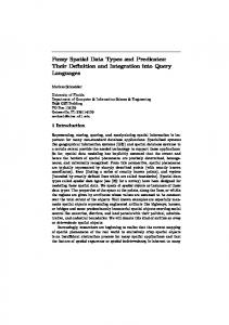
Operators of the last group take sets of objects as operands; some of them create new sets of objects as a result. The sum operator aggregates over the values of some spatial attribute of an object set and computes the geometric union of all these values. The closest operator yields that object of an object set whose spatial value is nearest to a spatial reference value. The decompose operator was already explained in Section 6.2; it multiplies each object of an object set according to the number of components of its spatial attribute value and adds this component as a new attribute. The overlay operator allows to superimpose one partition of the plane on another one and to combine them into area-disjoint regions. As described in Section 5.2, partitions are given as sets of objects with an attribute of a type in regions area-disjoint. The resulting set of objects contains one object for each new region obtained as the intersection of a region of the first partition with a region of the second partition.
−
27
−
overlay
Figure 15: Overlaying two partitions of the plane Note that it is not required that the plane is covered completely by the regions of a partition. Thus it is possible that a region of the first partition does not intersect any region of the second partition. In this case it will not be part of any new object6 (Figure 15). The fusion operator merges the values of a specified (set of) spatial attribute(s) on the basis of the equality of the values of another (set of) non-spatial attribute(s). For each group of equal non-spatial attribute values a (set of) new spatial value(s) is created as the geometric union of a set of spatial values of the group7. In Figure 16, a partition of districts with their land use is given. The task is to compute the regions with the same land use. Neighbour districts with the same land use are replaced by a single region, that is, their common boundary line is erased. Each of the hatched areas on the left is part of an object describing a district. On the right after the application of the fusion operator all areas belonging to the same group gi form a single regions value and are hatched in the same way. The signature for these operations is as follows:
∀ obj, obj1, obj2 in OBJ. ∀ geo, geo1, geo2 in GEO. ∀ area1, area2 in regions area-disjoint. ∀ datai in DATA. ∀ geoj in GEO. set(obj) × (obj → geo)
→ geo
sum
set(obj) × (obj → geo1) × geo2
→ set(obj)
closest
set(obj) × (obj → geo) × ident
→ set(o: OBJ)
decompose
set(obj1) × (obj1 → area1) × set(obj2) × (obj2 → area2) × ident set(obj) × (obj → datai)+ × (obj → geoj)+
→ set(o: OBJ)
overlay
→ set(o: OBJ)
fusion
Since the operations of this group deal with sets of objects, for their semantics definition the concepts of the object model interface are needed.
6
This corresponds to the standard join operation. If regions of one partition not intersecting a region of the other partition were in the result, it would be similar to an outer join.
7
The fusion operator could be extended to allow grouping also by spatial attributes. For efficient implementation this requires a capability of sorting by spatial data type values, which means the ROSE algebra would have to provide a “less-than” operator for each of the three SDTs imposing a linear order.
−
28
−
d1 d3 d6
g1
d5 d7
d2
g2
fusion
g1
g3
d9
g4
d8 d4
wheat
g3
g2
oats
barley
rye
Figure 16: Merging a partition of districts concerning the same land use For the definition of the sum operator let O = {o1, ..., on}, for n ≥ 0, be the operand set of objects and attr the attribute function yielding an SDT value for each object. union(...(union(attr(o1), attr(o2)), ...), attr(on)) fsum(O, attr) := ∅
if O ≠ ∅ otherwise
For the definition of the closest operator let O be the set of objects, attr the attribute function, and rv the reference value for which the nearest spatial value has to be calculated. Then fclosest(O, attr, rv) := {o ∈ O | ∀ o’ ∈ O : fdist(rv, attr(o)) ≤ fdist(rv, attr(o’))} The decompose operator has an unspecified result type in OBJ; hence in addition to its semantics function fdecompose it needs a type mapping τdecompose, as described in Section 5.1. When an operator alpha with a type mapping is used in a query and applied to some operands (say alpha(a, b, c)), then this will lead to a call of its semantics function falpha(a, b, c) during query execution. Additionally it will lead to a call of the type mapping function τalpha during query parsing; the type mapping function is called not with the actual operands (i.e., a, b, c) but instead with the actual types of these operands. These types can vary because of the polymorphic specification of operators which is the reason why type mappings are needed at all. The only exception to this rule are operands of type ident; for them not the type ident but the actual identifier is passed to the type mapping function. This is because the main purpose of such operands is the use in type mappings. fdecompose(O, attr, name) := {o ⊕ v | o ∈ O, v ∈ attr(o)} τdecompose(set(obj), (obj → geo), name) := obj ⊕ (name, geo) Hence each object is extended by one of the components of its spatial attribute; the new object type is an extension of the operand object type by a new attribute name of type geo. For example, the call in query Q4 (Section 6.2) “decompose(states, territory, basic_area)”would lead to the following calls
−
29
−
of semantics function and type mapping: fdecompose(states, territory, basic_area) τdecompose(set(state), (state → regions), basic_area) The overlay operator also needs a type mapping: foverlay(O1, attr1, O2, attr2, name) := {(o1 ⊗ o2) ⊕ v | ∃ o1 ∈ O1 ∃ o2 ∈ O2 : fintersects(attr1(o1), attr2(o2)) = true ∧ v = fintersection(attr1(o1), attr2(o2))} τoverlay(set(obj1), (obj1 → area1), set(obj2), (obj2 → area2), name) := (obj1 ⊗ obj2) ⊕ (name, new(regions area-disjoint)) Here the resulting object type is the product of the two operand types extended by a new attribute name of a new type in the kind regions area-disjoint. The fusion operator is not formally defined since it is only an abbreviation of a corresponding grouping operation, as described in Section 6. The semantics definition would rely on a formalization of the semantics of the grouping operation.
8 Integration with a DBMS Query Language: O2SQL/ROSE The purpose of this section is two-fold: (i) We show the integration of the ROSE algebra with one particular data model and query language, which further illustrates the concepts and requirements of the object model interface. (ii) We demonstrate the “expressive power” of the ROSE algebra (within the context of a query language) by showing some example queries. For the integration example we select O2 as one of the state-of-the-art object-oriented database systems with O2SQL as its current and future standard query language [Ba89, BaCD89, BaDK92, O293]. O2SQL is a functional language that deals with and allows to construct atomic values, tuples, sets and lists, provides operations on these structures, and allows one to define methods on classes. Flat as well as nested structures can be constructed, and all levels of a structure can be accessed. Elements of sets and lists and components of tuples may be of any type or class. The syntax of O2SQL has an SQL-like style through a select-from-where construct corresponding to the three algebraic operations projection, cartesian product, and selection, extended by object-oriented features. In the sequel we demonstrate the integration of our ROSE algebra with O2SQL by presenting example queries. The notations regarding class definitions and queries comply with the notations in [BaDK92, O293]. A few notational extensions are necessary. Examples are based on the following simple database which models spatial aspects of Germany. The keyword public means that components of a tuple structure are “visible” and can be accessed. class State public type tuple (name : string, territory : regions) end;
−
30
−
class City public type tuple (name : string, zipcode : integer, statistical_data : tuple ( foundation_date : integer, population : integer, unemployment_rate : real), municipal_area : regions) end; class Highway public type tuple (number : string, way : lines) end; class River public type tuple (name : string, route : lines) end; class District public type tuple (name : string, region : regions, land_use : string) end; A class is a description of a group of objects but not a persistent repository for them in a database. In O2 only objects associated with names are persistent. We therefore introduce for each class a named collection of objects: name Cities : set(City); name States : set(State); name Highways : set(Highway); name Rivers : set(River); name Districts : set(District); Spatial attributes are defined in the same way as attributes of standard data types, using the SDTs of the ROSE algebra. Note however, that we have compromised on the typing of regions attributes. In the example database, each of these attributes should really have its own type areai within the kind regionsarea-disjoint in order to be able to model partitions of the plane. Such a sophisticated typing is not available in O2. We will therefore assume that for the O2 integration the definition of the ROSE algebra is slightly changed so that all operators defined on areai types are defined on regions instead. This does not change the definition of syntax or semantics of these operators because any value of some type areai in regionsarea-disjoint is in fact a regions value; it just means that type checking cannot ensure any more that they are applied to partitions. The syntax of the spatial operations of the ROSE algebra in a query language is not prescribed by the signature of the operations but is part of the process of embedding the operations into the desired query language, i.e., dependent on the extended query language. Here, we select infix syntax for spatial predicates and the two operations plus and minus and a functional syntax for all other operations. Q1:
List the names and the land use of districts which are neighbors with the same land use. select from
tuple (dname1: d1.name, dname2: d2.name, land_use: d1.land_use) d1 in Districts, d2 in Districts where d1.region adjacent d2.region and d1.land_use = d2.land_use
−
31
−
All spatial predicates of the ROSE algebra (first group of spatial operations) can be used as selection criteria in the where clause, just like conventional predicates. The result of this query is a set of tuples each formed by the tuple constructor tuple. Components of tuples are accessed by the field extraction operator denoted by a dot. Hence here we have the facility of the OMI: Denote a data type value (within an object set iteration). Q2:
Which states are enclosed by which other states? select from
tuple (state1: s1, state2: s2) s1 in States, s2 in States where s1.territory encloses s2.territory
The result of the query is a set of tuples, each tuple being a pair of State objects. Q3:
Determine which highways cross which rivers and list their names, their geometries and their crossings. select
tuple (name: r.name, route: r.route, number: h.number, way: h.way, crossing: intersection (r.route, h.way)) from r in Rivers, h in Highways where r.route intersects h.way
Each tuple of the query result contains an attribute ‘crossing’ whose value is the intersection of a river and a highway value. (OMI: Extend objects by derived attribute values, allow naming of a new attribute.) Q4:
Associate with each state those cities lying inside that state. select
from
tuple (state: s, cities_in_state: select c from c in Cities where c.municipal_area inside s.territory) s in States
The result is a set of tuples, each tuple being a pair of a State object and a set of City objects whose geometry lies inside the geometry of the State object. Q5:
Which rivers form partially the boundary line of which states? In which parts do they agree? select from
tuple (rname: r.name, sname: s.name, border: common_border (s.territory, r.route)) s in States, r in Rivers where s.territory border_in_common r.route
Q6:
Compute the length of the river and highway network. length (sum (select attribute way from h in Highways) plus sum (select attribute route from r in Rivers))
Here we have introduced a first extension to O2SQL to fulfill the requirement of the OMI: Denote a collection of objects together with an attribute. The notation is “select attribute attr from s in S”
−
32
−
where attr is the name of the attribute and S the set of objects.8 This is analogous to the “column α from β” construct discussed in Section 6.2. It is interesting to observe that in this query first a single lines value is formed to which then the length function is applied. Using the sum aggregate function of O2 applicable to sets of reals, one might formulate the query as follows: sum (select length(h.way) from h in Highways) + sum (select length(r.route) from r in Rivers) Actually the result will only be the same if no two highways use the same piece of the highway network. But a more important issue to be discussed here is the view of aggregate functions. The sum aggregate function of O2 used in this last example is applied to a set of values. In contrast, the only aggregate function of the ROSE algebra (sum) is applied to a set of objects with a spatial attribute. The rationale behind this is to keep the type system of the object model interface as simple as possible. For example, in the relational model sets of values are not available. The ROSE algebra only assumes that collections of objects and atomic values exist. Q7:
Calculate the perimeter of Bavaria (class State is assumed to describe states within Germany). perimeter (element (select s.territory from s in States where s.name = “Bavaria”))
The O2SQL element operator extracts the unique element of a singleton set. This is exactly the facility “denote a data type value (without object set iteration)” of the OMI. The expression “element ...” denotes the territory of Bavaria. Q8:
Calculate the region outside Bavaria where wheat is cultivated. sum (select attribute region from d in Districts where d.land_use = “wheat”) minus element (select s.territory from s in States where s.name = “Bavaria”)
This query yields an atomic spatial value. Q9:
Determine all cities that are located in areas which are completely enclosed by highways. select c from c in Cities where c.municipal_area inside interior (sum (select attribute way from h in Highways))
This query yields a set of City objects fulfilling the where condition. Q10: Check if the highways form a connected network. no_of_components (sum (select attribute way from h in Highways)) = 1 8
For the SQL embedding in Section 6.2 we have used a keyword “column”. This seemed to fit with SQL which also speaks of “tables” rather than relations. For O2 which uses terms like “tuple”, a keyword “attribute” appears adequate. Of course, this is just a matter of taste.
−
33
−
Q11: List the name(s) of the highway(s) being closest to Munich. define Munich as element (select c.municipal_area from c in Cities where c.name = “Munich”); select from
h.number h in closest (select attribute way from h in Highways, Munich)
In the first step a named query of O2 defines Munich as a regions value. This is the facility “allow naming of an SDT value” of the OMI. The closest operator takes as operands a class or any other homogeneous set of objects together with a spatial attribute defined on that object type, and a spatial reference value (in this case Munich). It returns a set of objects which can be used in a query at all those positions where a set expression is allowed. Q12: Determine the component regions of the state Schleswig-Holstein (which consists of a main land area as well as several islands in the North Sea). select from
s.component s in decompose into component select attribute territory from s in States where s.name = “Schleswig-Holstein”
The decompose operator has three arguments: a class or any other homogeneous set of objects, an SDT attribute to be decomposed, and a name for the new attribute resulting from decomposition. The query yields a set of regions values. Here we have introduced a second extension to O2SQL to offer the facility “allow naming of a new attribute” of the OMI, using a phrase “into attr”, as in Section 6.2. Q13: Partition the state Bavaria with respect to the districts of land use. overlay into districts_within_Bavaria (select attribute territory from s in States where s.name = “Bavaria”, select attribute region from d in Districts) The result is a set of objects with a new attribute “districts_within_Bavaria”. Each partition for the overlay is given as a set of objects with a regions attribute. Q14: Compute the regions of the same land use. fusion (Districts; land_use; region) The fusion operator requires three arguments which are syntactically separated by semicolons: a set of objects, a list of non-spatial attributes used for grouping, and a list of spatial attributes used for geometric union. In the query above the District objects are grouped according to equal land use and for each group the geometric union of the regions values of the “region” attribute is formed. O2SQL offers a grouping operator group so that the query can be formulated without an explicit fusion operator:
− group with
34
−
d in Districts by (land_use: d.land_use) (region: sum (select attribute p.region from p in partition))
Here the group operator is applied to a set of District objects. It groups District objects by values of their “land_use” attribute and produces for each group one result tuple with two attributes. The first attribute “land_use” receives the value of the “land_use” attribute of the group; the second attribute “region” is determined in the with-clause by an expression which computes for each group the geometric union of the “region” attribute values. One can refer to the current group by a keyword partition.
9 Conclusions In this paper and the companion paper [GüS93] we have defined the ROSE algebra, a system of realmbased spatial data types. After the geo-relational algebra [Gü88a] which was implemented in the Gral system9 [Gü89, BeG92] this is a second attempt to define a spatial algebra for database systems and in some sense it represents what we have learned in the meantime. In closing, let us summarize the highlights of the ROSE algebra. It may also be interesting to compare to the geo-relational algebra (in the sequel geo-algebra for short). General types and operations. The ROSE algebra has very general data types to represent points, lines, and regions in the plane. For example, it is now possible to represent the whole area of a state including islands or separate land areas in a single regions value, or a complete highway network in a single lines value. On the one hand, this generality makes the spatial objects and operations conceptually more difficult, requires a quite elaborate system of definitions, and also needs more effort in the implementation. This is why in the geo-algebra a decision was made to deal only with simple polygons and single-component objects. On the other hand, the generality is needed in applications (with Gral this became obvious when the German state of Niedersachsen had to be represented which encloses - as a hole - the state of Bremen). We feel that through the several layers of definitions of the ROSE algebra we have managed the complexity. Apart from the better capability to model spatial objects, an important benefit is that the types are now closed under set operations of the underlying point sets - for any type one can form union, difference (plus, minus) or aggregate over its values (sum) which makes the rather complex fusion operation [ScV89, GaNT91] a simple byproduct of grouping. Also, all operations are now defined in the most general way (e.g. the closest operation is available for all spatial types). In contrast, in the geo-algebra it was not possible to define a difference operator on regions since it would have led to holes, and intersection had to be defined as a relation operation because a resulting set of intersection values could not be represented as a single SDT value. Rigorous definition. The carrier sets of the types and the semantics of all operations have been defined completely, down to the level of simple arithmetic primitives on integers. As a result, there is no ambiguity for a programmer about the precise meaning of operations or about allowed structures. We feel this is very important because when dealing with complex spatial structures invariably questions about special cases come up like “Is it allowed that the boundary of a hole in a region touches the outer 9
The second author took part in this implementation effort.
−
35
−
boundary?” or “Qualify two adjacent regions as intersecting?” The ROSE algebra definition gives precise answers to all such questions to an implementor and, if not to end users, at least to people writing manuals for end users. Numerical robustness, finite resolution. The underlying realm provides the ROSE algebra with a discrete basis and shields it from all problems of numerical robustness. Integer coordinates can be used for the representation of SDT values; critical operations like testing whether points lie on the border of regions become feasible. In contrast, in the geo-algebra operations like meets or common_border were omitted, because - with real numbers representing coordinates of SDT values - it was not clear how these operations could be implemented in a numerically robust way. The discrete basis also greatly simplifies the implementation of geometric algorithms for the operations. For example, to implement common_border one can keep for each lines or regions value its defining segments in (x, y)-lexicographic order and then simply scan the two lists in parallel. Many operations can be implemented by plane-sweep algorithms [NiP82, BeO79] which are simplified here because no intersection points need to be computed; all sweep stations are known beforehand and one does not need a dynamic structure to maintain the ordered list of sweep stations. Data model independence, clean object model interface. The ROSE algebra is not tied to any particular data model but can cooperate with many models and query languages. This might have been achieved in a trivial way by omitting all operations manipulating objects (like closest, overlay) and not caring how the results of geometric operations can be used in the DBMS. Instead, we have defined an object model interface and investigated quite carefully the issues arising with the integration of the ROSE algebra into a query language. Section 8 has demonstrated that a nice integration with, for example, an object-oriented model and query language can be achieved. To our knowledge, this is the first time that the problem of interfacing a general purpose query language with a complex application-specific sublanguage has been examined in some detail. Such interfaces will be important for cooperative database systems using external computation services [ScW91]. Open Problems and Future Work Implementation of the ROSE algebra. Data structures for the three SDTs and procedures for all operations except for dist and the set-manipulating operations of the last group (Section 7.4) have been realized [Ri94] and are available as a module library written in Modula-2. The implementation of operations makes heavy use of the following three techniques: (i) scan or parallel scan of the halfsegment sequence10 of one or two objects, (ii) plane-sweep, and (iii) graph algorithms [Ri94]. Algorithms and practical aspects of the implementation will be described in a forthcoming paper [GüRS95]. As a next step, we plan to encapsulate this implementation within a “data type extension package” and then to connect it to the Gral system as well as to another query processor called SECONDO. A component that allows to represent a realm and which offers realm operations (updates with redrawing, described in [GüS93]) is almost finished. The points and segments of a realm are stored in an LSD-tree [HeSW89]. For the problems of interfacing realms and database systems see [GüS93]. 10 For
a lines or regions value, its halfsegment sequence contains each segment of the object twice, once for the left and once for the right end point, called the dominating point for this segment. The halfsegment sequence is ordered xylexicographically by dominating points.
−
36
−
Some problems remain with the realm-based approach and need to be further investigated: Invariance under redrawing. We are not satisfied with the fact that some of the numeric ROSE operations (length, area, etc.) yield slightly different results before and after a redrawing due to an update of the realm. Whereas we feel that slight numerical errors are tolerable in contrast to topological errors, this may also lead to “discrete errors”. For example, when a collection of objects is sorted by area of its regions, the order may change through a realm update. Perhaps a definition of these operations can be found that is sufficiently consistent with the geometry of the objects, but invariant under redrawing. Objects and operations violating realm closure. One is still interested in spatial objects that are not part of the given realm. For example, it should be possible to draw interactively a region and then to use it in a query. The new region cannot directly be compared with realm-based objects. One possible strategy might be to insert this region temporarily into the realm and to remove it again when the query has been processed. There may be other solutions. We have so far restricted attention to operations that are closed with respect to the underlying realm, but there are also interesting operations that leave the given realm, for example, construction of a Voronoi diagram, a convex hull, or of a buffer zone around a spatial object. One should study how these can be accommodated. One strategy might be to create a new realm for the new spatial values, select a set of SDT values in the database that might interact with the new geometries and create another “small” realm for them, and then use a “merge” operation on realms to compute all intersections. Acknowledgments The authors thank the referees who read the manuscript very carefully and provided a large number of detailed questions and suggestions that helped to improve the presentation. Thanks also to Andrew Frank, Michel Scholl, and Agnès Voisard for their comments. References [Ba89]
Bancilhon F., Query Languages for Object-Oriented Database Systems: Analysis and a Proposal. Proc. BTW (Datenbanksysteme in Büro, Technik und Wissenschaft, Zürich 1989), Springer, InformatikFachberichte 204, 1-18.
[BaCD89]
Bancilhon F., S. Cluet, and C. Delobel, A Query Language for the O2 Object-Oriented Database System. Proc. of the 2nd Workshop on Database Programming Languages (Salishan, Oregon), 1989.
[BaDK92]
Bancilhon, F., C. Delobel, and P. Kanellakis, The O2Book. Morgan-Kaufmann, San Mateo, CA, 1992.
[BeG92]
Becker, L., and R.H. Güting, Rule-Based Optimization and Query Processing in an Extensible Geometric Database System. ACM Transactions on Database Systems 17 (1992), 247-303.
[BeO79]
Bentley, J.L., and T. Ottmann, Algorithms for Reporting and Counting Geometric Intersections. IEEE Trans. on Computers C-28 (1979), 643-647.
[EgFJ89]
Egenhofer, M.J., A. Frank, and J.P. Jackson, A Topological Data Model for Spatial Databases. Proc. SSD 89 (Santa Barbara, California), 1989, 271-286.
[FrK86]
Frank A., and W. Kuhn, Cell Graphs: A Provable Correct Method for the Storage of Geometry. Proc. of the 3rd Int. Symposium on Spatial Data Handling, 1986, 411-436.
[GaNT91]
Gargano, M., E. Nardelli, and M. Talamo, Abstract Data Types for the Logical Modeling of Complex Data. Information Systems 16, 5 (1991), 565-584.
[GrY86]
Greene, D., and F. Yao, Finite-Resolution Computational Geometry. Proc. 27th IEEE Symp. on Foundations of Computer Science, 1986, 143-152.
−
37
−
[Gü88a]
Güting, R.H., Geo-Relational Algebra: A Model and Query Language for Geometric Database Systems. Proc. of the Intl. Conf. on Extending Database Technology (Venice, Italy), 1988, 506-527.
[Gü88b]
Güting, R.H., Modeling Non-Standard Database Systems by Many-Sorted Algebras. Fachbereich Informatik, Universität Dortmund, Report 255, 1988.
[Gü89]
Güting, R.H., Gral: An Extensible Relational Database System for Geometric Applications. Proc. of the 15th Intl. Conf. on Very Large Databases (Amsterdam, The Netherlands), 1989, 33-44.
[Gü93]
Güting, R.H., Second-Order Signature: A Tool for Specifying Data Models, Query Processing, and Optimization. Proc. ACM SIGMOD Conf. (Washington, USA), 1993, 277-286.
[GüRS95]
Güting, R.H., T. de Ridder, and M. Schneider, Implementation of the ROSE Algebra. Manuscript in Preparation, 1995.
[GüS93]
Güting, R.H., and M. Schneider, Realms: A Foundation for Spatial Data Types in Database Systems. Proc. of the 3rd Intl. Symposium on Large Spatial Databases (Singapore), 1993, 14-35.
[HeSW89]
Henrich, A., H.-W. Six, and P. Widmayer, The LSD Tree: Spatial Access to Multidimensional Point- and Non-Point-Objects. Proc. of the 15th Intl. Conf. on Very Large Data Bases (Amsterdam, The Netherlands), 45-53.
[JoC88]
Joseph, T., and A. Cardenas, PICQUERY: A High Level Query Language for Pictorial Database Management. IEEE Trans. on Software Engineering 14 (1988), 630-638.
[LeR89]
Lécluse, C., and P. Richard, The O2 Database Programming Language. Proc. 15th Intl. Conf. on Very Large Data Bases (Amsterdam, The Netherlands), 1989, 411-422.
[LiN87]
Lipeck, U., and K. Neumann, Modelling and Manipulating Objects in Geoscientific Databases. Proc. 5th Intl. Conf on the Entity-Relationship Approach (Dijon, France, 1986), 1987, 67-86.
[NiP82]
Nievergelt, J., and F.P. Preparata, Plane-Sweep Algorithms for Intersecting Geometric Figures. Communications of the ACM 25 (1982), 739-747.
[OrM88]
Orenstein, J., and F. Manola, PROBE Spatial Data Modeling and Query Processing in an Image Database Application. IEEE Trans. on Software Engineering 14 (1988), 611-629.
[O293]
The O2 User’s Manual, Version 4.1. O2 Technology, 1993.
[Ri94]
de Ridder, T., Die ROSE-Algebra: Implementierung geometrischer Datentypen und Operationen für erweiterbare Datenbanksysteme (The ROSE Algebra: Implementation of Geometric Data Types and Operations for Extensible Database Systems). Fernuniversität Hagen, Fachbereich Informatik, Diplomarbeit (Master Thesis), 1994.
[RoFS88]
Rossopoulos, N., C. Faloutsos, and T. Sellis, An Efficient Pictorial Database System for PSQL. IEEE Trans. on Software Engineering 14 (1988), 639-650.
[ScW91]
Schek, H.J., and G. Weikum, Erweiterbarkeit, Kooperation, Föderation von Datenbanksystemen (Extensibility, Cooperation, Federation of Database Systems). Proc. Datenbanksysteme in Büro, Tecnnik und Wissenschaft, Kaiserslautern,1991, Springer, Informatik-Fachberichte 270, 38-71.
[ScV89]
Scholl, M., and A. Voisard, Thematic Map Modeling. Proc. SSD 89, (Santa Barbara, California), 1989, 167-190.
[SvH91]
Svensson, P., and Z. Huang, Geo-SAL: A Query Language for Spatial Data Analysis. Proc. SSD 91 (Zürich, Switzerland), 1991, 119-140.
[To90]
Tomlin, C.D., Geographic Information Systems and Cartographic Modeling. Prentice Hall, 1990.
[Vo92]
Voisard, A., Bases de données géographiques: du modèle de données à l’interface utilisateur. Ph.D. Thesis, University of Paris-Sud (Centre d’Orsay), 1992.
−
38
−
Appendix: Definition Layers For Realm-Based Spatial Data Types Objects: ROSE Algebra Operations
Operations: =, ≠, inside, edge_inside, vertex_inside, area_disjoint, edge_disjoint, disjoint, intersects, meets, adjacent, encloses, on_border_of, border_in_common, intersection, plus, minus, common_border, vertices, contour, interior, count, dist, diameter, length, area, perimeter, sum, closest, decompose, overlay, fusion
Objects: Spatial Data Types and Spatial Algebra Primitives
Realms, Realm-Based Structures and RealmBased Primitives
Robust Geometric Primitives
Integer Arithmetic (see [GüS93])
points, lines, regions
points, lines, regions
Operations: union, intersection, difference, (area-)inside, edge-inside, vertex-inside, area-disjoint, edge-disjoint, (vertex-)disjoint, adjacent, meet, intersect, encloses, on_border_of, border_in_common
Objects:
R-point, R-segment; R-cycle, R-face, R-unit, R-block
Operations: on, in, out, (area-)inside, edge-inside, vertex-inside, areadisjoint, edge-disjoint, (vertex-)disjoint, adjacent, meet, encloses, intersect, dist, area
Objects:
N-point, N-segment
Operations: =, meet, overlap, intersect, disjoint, on, in, intersection, parallel, aligned
Objects:
integers in the range [-2n3, 2n3] (n integer grid size)
Operations:
+, -, ∗, div, mod, =, ≠,