REASONING ABOUT DATA REPETITIONS WITH COUNTER

Logical Methods in Computer Science Vol. 12(3:1)2016, pp. 1–55 www.lmcs-online.org

Submitted Published

Mar. 2, 2015 Aug. 1, 2016

REASONING ABOUT DATA REPETITIONS WITH COUNTER SYSTEMS ∗ ´ STEPHANE DEMRI a , DIEGO FIGUEIRA b , AND M. PRAVEEN c a

LSV, ENS Cachan, CNRS, Universit´e Paris-Saclay, 94235 Cachan, France

b

LaBRI, CNRS, 33405 Talence, France

c

CMI, Chennai, India

Abstract. We study linear-time temporal logics interpreted over data words with multiple attributes. We restrict the atomic formulas to equalities of attribute values in successive positions and to repetitions of attribute values in the future or past. We demonstrate correspondences between satisfiability problems for logics and reachability-like decision problems for counter systems. We show that allowing/disallowing atomic formulas expressing repetitions of values in the past corresponds to the reachability/coverability problem in Petri nets. This gives us 2expspace upper bounds for several satisfiability problems. We prove matching lower bounds by reduction from a reachability problem for a newly introduced class of counter systems. This new class is a succinct version of vector addition systems with states in which counters are accessed via pointers, a potentially useful feature in other contexts. We strengthen further the correspondences between data logics and counter systems by characterizing the complexity of fragments, extensions and variants of the logic. For instance, we precisely characterize the relationship between the number of attributes allowed in the logic and the number of counters needed in the counter system.

1. Introduction Words with multiple data. Finite data words [Bou02] are ubiquitous structures that include timed words, runs of counter automata or runs of concurrent programs with an unbounded number of processes. These are finite words in which every position carries a label from a finite alphabet and a data value from some infinite alphabet. More generally, structures over an infinite alphabet provide an adequate abstraction for objects from several domains: for example, infinite runs of counter automata can be viewed as infinite data words, finite arrays are finite data words [AvW12], finite data trees model XML 2012 ACM CCS: [Theory of computation]: Logic; Formal languages and automata theory; Theory and algorithms for application domains. Key words and phrases: data-word, counter systems, LTL. ∗ Complete version of [DFP13]. Work supported by project REACHARD ANR-11-BS02-001, and FET-Open Project FoX, grant agreement 233599. M. Praveen was supported by the ERCIM “Alain Bensoussan” Fellowship Programme.

l

LOGICAL METHODS IN COMPUTER SCIENCE

DOI:10.2168/LMCS-12(3:1)2016

c S. Demri, D. Figueira, and M. Praveen

CC

Creative Commons

2

S. DEMRI, D. FIGUEIRA, AND M. PRAVEEN

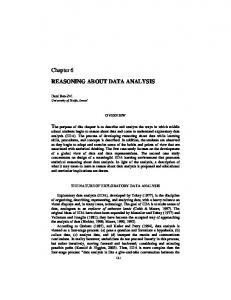
documents with attribute values [Fig10] and so on. A wealth of specification formalisms for data words (or slight variants) has been introduced stemming from automata, see e.g. [NSV04, Seg06], to adequate logical languages such as first-order logic [BDM+ 11, Dav09] or temporal logics [LP05, KV06, Laz06, Fig10, KSZ10, Fig11] (see also a related formalism in [Fit02]). Depending on the type of structures, other formalisms have been considered such as XPath [Fig10] or monadic second-order logic [BCGK12]. In full generality, most formalisms lead to undecidable decision problems and a well-known research trend consists of finding a good trade-off between expressiveness and decidability. Restrictions to regain decidability are protean: bounding the models (from trees to words for instance), restricting the number of variables, see e.g. [BDM+ 11], limiting the set of the temporal operators or the use of the data manipulating operator, see e.g. [FS09, DDG12]. As far as classes of automata for data languages are concerned, other questions arise related to closure properties or to logical characterisations, see e.g. [BDM+ 11, BL10, KST12]. Moreover, interesting and surprising results have been exhibited about relationships between logics for data words and counter automata (including vector addition systems with states) [BDM+ 11, DL09, BL10], leading to a first classification of automata on data words [BL10, Bol11]. This is why logics for data words are not only interesting for their own sake but also for their deep relationships with data automata or with counter automata. Herein, we pursue further this line of work and we work with words in which every position contains a vector of data values. Motivations. In [DDG12], a decidable linear-time temporal logic interpreted over (finite or infinite) sequences of variable valuations (understood as words with multiple data) is introduced in which the atomic formulae are of the form either x ≈ Xi y or x ≈ h>?iy. The formula x ≈ Xi y states that the current value of variable x is the same as the value of y i steps ahead (local constraint) whereas x ≈ h>?iy states that the current value of x is repeated in a future value of y (future obligation). Such atomic properties can be naturally expressed with a freeze operator that stores a data value for later comparison, and in [DDG12], it is shown that the satisfiability problem is decidable with the temporal operators in {X, X−1 , U, S}. The freeze operator allows to store a data value in a register and then to test later equality between the value in the register and a data value at some other position. This is a powerful mechanism but the logic in [DDG12] uses it in a limited way: only repetitions of data values can be expressed and it restricts very naturally the use of the freeze operator. The decidability result is robust since it holds for finite or infinite sequences, for any set of MSO-definable temporal operators and with the addition of atomic formulas of the form x ≈ h>?i−1 y stating that the current value of x is repeated in a past value of y (past obligation). Decidability can be shown either by reduction into FO2 (∼, = CLTLXF,XF

3

[DDG12]

(1 attribute) LRV

LRV> = CLTLXF [DDG12]

Figure 1: Placing LRV and variants in the family of data logics two fragments BD-LTL− and BD-LTL+ of that richer logic have been introduced and shown to admit 2expspace-complete satisfiability problems. Forthcoming logic LRV> is shown in [DHLT14] to be strictly less expressive than BD-LTL+ . Our main motivation is to investigate logics that express repetitions of values, revealing the correspondence between expressivity of the logic and reachability problems for counter machines, including well-known problems for Petri nets. This work can be seen as a study of the precision with which counting needs to be done as a consequence of having a mechanism for demanding “the current data value is repeated in the future/past” in a logic. Hence, this is not the study of yet another logic, but of a natural feature shared by most studied logics on data words [DDG12, BDM+ 11, DL09, FS09, KSZ10, Fig10, Fig11]: the property of demanding that a data value be repeated. We consider different ways in which one can demand the repetition of a value, and study the repercussion in terms of the “precision” with which we need to count in order to solve the satisfiability problem. Our measurement of precision here distinguishes the reachability versus the coverability problem for Petri nets and the number of counters needed as a function of the number of variables used in the logic. Our contribution. We introduce the linear-time temporal logic LRV (“Logic of Repeating Values”) interpreted over finite words with multiple data, equipped with atomic formulas of the form either x ≈ Xi y or x ≈ hφ?iy [resp. x 6≈ hφ?iy], where x ≈ hφ?iy [resp. x 6≈ hφ?iy] states that the current value of x is repeated [resp. is not repeated] in some future value of y in a position where φ holds true. When we impose φ = >, the logic introduced in [DDG12] is obtained and it is denoted by LRV> (a different name is used in [DDG12], namely CLTLXF ). Note that the syntax for future obligations is freely inspired from propositional dynamic logic PDL with its test operator ‘?’. Even though LRV contains the past-time temporal operators X−1 and S, it has no past obligations. We write PLRV to denote the extension of LRV with past obligations of the form x ≈ hφ?i−1 y or x 6≈ hφ?i−1 y. Figure 1 illustrates how LRV and variants are compared to existing data logics. Our main results are listed below. i. We begin where [DDG12] stopped: the reachability problem for Petri nets is reduced to the satisfiability problem of PLRV (i.e., the logic with past obligations). ii. Without past obligations, the satisfiability problem is much easier: we reduce the satisfiability problem of LRV> and LRV to the control-state reachability problem for VASS, via a detour to a reachability problem on gainy VASS. But the number of counters in the VASS is exponential in the number of variables used in the formula. This gives us a 2expspace upper bound. iii. The exponential blow up mentioned above is unavoidable: we show a polynomial-time reduction in the converse direction, starting from a linear-sized counter machine (without

4


zero tests) that can access exponentially many counters. This gives us a matching 2expspace lower bound. iv. Several augmentations to the logic do not alter the complexity: we show that complexity is preserved when MSO-definable temporal operators are added or when infinite words with multiple data are considered. v. The power of nested testing formulas: we show that the complexity of the satisfiability problem for LRV> reduces to pspace-complete when the number of variables in the logic is bounded by a constant, while the complexity of the satisfiability of LRV does not reduce even when only one variable is allowed. Recall that the difference between LRV> and LRV is that the later allows any φ in x ≈ hφ?iy while the former restricts φ to just >. vi. The power of pairs of repeating values: we show that the satisfiability problem of LRV> augmented with hx, yi ≈ h>?ihx0 , y0 i (repetitions of pairs of data values) is undecidable, even when hx, yi ≈ h>?i−1 hx0 , y0 i is not allowed (i.e., even when past obligations are not allowed). vii. Implications for classical logics: we show a 3expspace upper bound for the satisfiability problem for forward-EMSO2 (+1, 0 and σ, i − 1 |= φ σ, i |= φUφ0 iff there is i ≤ j < |σ| such that σ, j |= φ0 and for every i ≤ l < j, we have σ, l |= φ σ, i |= φSφ0 iff there is 0 ≤ j ≤ i such that σ, j |= φ0 and for every j < l ≤ i we have σ, l |= φ. We write σ |= φ if σ, 0 |= φ. We use the standard derived temporal operators (G, F, F−1 , . . . ), and derived Boolean operators (∨, ⇒, . . . ) and constants >, ⊥. We also use the notation Xi x ≈ Xj y as an abbreviation for the formula Xi (x ≈ Xj−i y) (assuming without any loss of generality that i ≤ j). Similarly, Xj y ≈ x is an abbreviation for x ≈ Xj y. Given a set of temporal operators O definable from those in {X, X−1 , S, U} and a natural number k ≥ 0, we write LRVk (O) to denote the fragment of LRV restricted to formulas with temporal operators from O and with at most k variables. The satisfiability problem for LRV (written SAT(LRV)) is to check for a given LRV formula φ, whether there exists a model σ such that σ |= φ. Note that there is a logarithmic-space reduction from the satisfiability problem for LRV to its restriction where atomic formulas of the form x ≈ Xi y satisfy i ∈ {0, 1} (at the cost of introducing new variables). Let PLRV be the extension of LRV with additional atomic formulas of the form x ≈ hφ?i−1 y and x 6≈ hφ?i−1 y. The satisfaction relation is extended as follows: σ, i |= x ≈ hφ?i−1 y iff there is 0 ≤ j < i such that σ(i)(x) = σ(j)(y) and σ, j |= φ σ, i |= x 6≈ hφ?i−1 y iff there is 0 ≤ j < i such that σ(i)(x) 6= σ(j)(y) and σ, j |= φ. We write LRV> [resp. PLRV> ] to denote the fragment of LRV [resp. PLRV] in which atomic formulas are restricted to x ≈ Xi y and x ≈ h>?iy [resp. x ≈ Xi y, x ≈ h>?iy and x ≈ h>?i−1 y]. These are precisely the fragments considered in [DDG12] and shown decidable by reduction into the reachability problem for Petri nets. Proposition 2.1. [DDG12]

6


(I) Satisfiability problem for LRV> is decidable (by reduction to the reachability problem for Petri nets). (II) Satisfiability problem for LRV> restricted to a single variable is pspace-complete. (III) Satisfiability problem for PLRV> is decidable (by reduction to the reachability problem for Petri nets). In [DDG12], there are no reductions in the directions opposite to (I) and (III). The characterisation of the computational complexity for the satisfiability problems for LRV and PLRV remained unknown so far and this will be a contribution of the paper. 2.2. Properties. In the table below, we justify our choices for atomic formulae by presenting several abbreviations (with their obvious semantics). By contrast, we include in LRV both x ≈ hφ?iy and x 6≈ hφ?iy when φ is an arbitrary formula since there is no obvious way to express one with the other. Abbreviation

Definition i times

x 6≈ x≈

Xi y

X−i y

x 6≈ X−i y x 6≈ h>?iy x 6≈ h>?i−1 y

¬(x ≈

Xi y)

i times

z }| { ∧ X···X>

}| { z X−1 · · · X−1 (y ≈ Xi x) i times

}| { z ¬(x ≈ X−i y) ∧ X−1 · · · X−1 > (x 6≈ Xy) ∨ X((y ≈ Xy)U(y 6≈ Xy)) (x 6≈ X−1 y) ∨ X−1 ((y ≈ X−1 y)S(y 6≈ X−1 y))

Models for LRV can be viewed as finite data words in (Σ × D)∗ , where Σ is a finite alphabet and D is an infinite domain. E.g., equalities between dedicated variables can simulate that a position is labelled by a letter from Σ; moreover, we may assume that the data values are encoded with the variable x. Let us express that whenever there are i < j such that i and j [resp. i + 1 and j + 1, i + 2 and j + 2] are labelled by a [resp. a0 , a00 ], σ(i + 1)(x) 6= σ(j + 1)(x). This can be stated in LRV by: G(a ∧ X(a0 ∧ Xa00 ) ⇒ X¬(x ≈ hX−1 a ∧ a0 ∧ Xa00 ?ix)).

This is an example of key constraints, see e.g. [NS11, Definition 2.1] and the current paper contains also numerous examples of properties that can be captured by LRV. 2.3. Basics on VASS. A vector addition system with states is a tuple A = hQ, C, δi where Q is a finite set of control states, C is a finite set of counters and δ is a finite set of transitions in Q × ZC × Q. A configuration of A is a pair hq, vi ∈ Q × NC . We write hq, vi → − hq 0 , v0 i if ∗ there is a transition (q, u, q 0 ) ∈ δ such that v0 = v + u. Let → − be the reflexive and transitive closure of → − . The reachability problem for VASS (written Reach(VASS)) consists of checking ∗ whether hq0 , v0 i → − hqf , vf i, given two configurations hq0 , v0 i and hqf , vf i. The reachability problem for VASS is decidable but all known algorithms [May84, Kos82, Lam92, Ler11] take non-primitive recursive space in the worst case. The best known lower bound is expspace [Lip76, Esp98] whereas a first upper bound has been recently established in [LS15]. The ∗ control state reachability problem consists in checking whether hq0 , v0 i → − hqf , vi for some

REASONING ABOUT DATA REPETITIONS WITH COUNTER SYSTEMS

7

v ∈ NC , given a configuration hq0 , v0 i and a control state qf . This problem is known to be expspace-complete [Lip76, Rac78]. The relation → − denotes the one-step transition in a perfect computation. In the paper, we need to introduce computations with gains or with losses. We define below the variant relations → − gainy and → − lossy . We write hq, vi → − gainy hq 0 , v0 i 0 0 C 0 if there is a transition (q, u, q ) ∈ δ and w, w ∈ N such that v w, w = w + u and ∗ − gainy be the reflexive and transitive closure of → w0 v0 . Let → − gainy . Similarly, we write hq, vi → − lossy hq 0 , v0 i if there is a transition (q, u, q 0 ) ∈ δ and w, w0 ∈ NC such that w v, ∗ − lossy be the reflexive and transitive closure of → w0 = w + u and v0 w0 . Let → − lossy . Counter automata with imperfect computations such as lossy channel systems [AJ96, FS01], lossy counter automata [May03] or gainy counter automata [Sch10b] have been intensively studied (see also [Sch10a]). In the paper, imperfect computations are used with VASS in Section 4. 3. The Power of Past: From Reach(VASS) to SAT(PLRV) While [DDG12] concentrated on decidability results, here we begin with a hardness result. When past obligations are allowed as in PLRV, SAT(PLRV) is equivalent to the very difficult problem of reachability in VASS (see recent developments in [LS15]). Combined with the result of the next section where we prove that removing past obligations leads to a reduction into the control state reachability problem for VASS, this means that reasoning with past obligations is probably much more complicated. Theorem 3.1. There is a polynomial-space reduction from Reach(VASS) into SAT(PLRV). The proof of Theorem 3.1 is analogous to the proof of [BDM+ 11, Theorem 16] except that properties are expressed in PLRV instead of being expressed in FO2 (∼, that preserves satisfiability: there is a model σ such that σ |= ϕ iff there is a model σ 0 such that σ 0 |= ϕ0 . We give the reduction in two steps. First, we eliminate formulas with inequality tests of the form x 6≈ hψ?iy using only positive tests of the form x ≈ hψ?iy. We then eliminate formulas of the form x ≈ hψ?iy, using only formulas of the form x ≈ h>?iy. Although both reductions share some common structure, they use independent coding strategies, and exploit different features of the logic; we therefore present them separately. We first show how to eliminate all formulas with inequality tests of the form x 6≈ hψ?iy. Let LRV≈ be the logic LRV where there are no appearances of formulas of the form x 6≈ hψ?iy; and let PLRV≈ be PLRV without x 6≈ hψ?iy or x 6≈ hψ?i−1 y. Henceforward, vars(ϕ) denotes the set of all variables in ϕ, and subhi(ϕ) the set of all subformulas ψ such that x ≈ hψ?iy or x 6≈ hψ?iy appears in ϕ for some x, y ∈ vars(ϕ). In both reductions we make use of the following easy lemma. Lemma 4.1. There is a polynomial-time satisfiability-preserving translation t : LRV → LRV [resp. t : LRV≈ → LRV≈ ] such that for every ϕ and ψ ∈ subhi(t(ϕ)), we have subhi(ψ) = ∅. Proof. This is a standard reduction. Indeed, given a formula ϕ with subformula x ≈ hψ?iy, ϕ is satisfiable iff G(ψ ⇔ xnew ≈ ynew ) ∧ ϕ[x ≈ hψ?iy ← x ≈ hxnew ≈ ynew ?iy] is satisfiable, where xnew , ynew 6∈ vars(ϕ), and ϕ[x ≈ hψ?iy ← x ≈ hxnew ≈ ynew ?iy] is the result of replacing every occurrence of x ≈ hψ?iy by x ≈ hxnew ≈ ynew ?iy in ϕ. Similarly, given a formula ϕ with subformula x 6≈ hψ?iy, ϕ is satisfiable iff G(ψ ⇔ xnew ≈ ynew ) ∧ ϕ[x 6≈ hψ?iy ← x 6≈ hxnew ≈ ynew ?iy] is satisfiable. We need to apply these replacements repeatedly, at most a polynomial number of times if we apply it to the innermost occurrences. Proposition 4.2 (from LRV to LRV≈ ). There is a polynomial-time reduction from SAT(LRV) into SAT(LRV≈ ); and from SAT(PLRV) into SAT(PLRV≈ ). Proof. For every ϕ ∈ LRV, we compute ϕ0 ∈ LRV≈ in polynomial time, which preserves satisfiability. The variables of ϕ0 consist of all the variables of ϕ, plus: a distinguished variable k, and variables v≈ y,ψ , vx6≈hψ?iy for every subformula ψ of ϕ and variables x, y of ϕ. The variables vx6≈hψ?iy ’s will be used to get rid of 6≈ in formulas of the form x 6≈ hψ?iy, and the variables v≈ y,ψ ’s to treat formulas of the form ¬(x 6≈ hψ?iy). Finally, k is a special variable, which has a constant value, different from all the values of the variables of ϕ. Assume ϕ is in negation normal form. Note that each positive occurrence of x 6≈ hψ?iy can be safely replaced with x 6≈ vx6≈hψ?iy ∧ vx6≈hψ?iy ≈ hψ?iy. Indeed, the latter formula implies the former, and it is not difficult to see that whenever there is a model for the former formula, there is also one for the latter. On the other hand, translating formulas of the form ¬(x 6≈ hψ?iy) is more involved as these implicate some form of universal quantification. For treating these formulas, we use the variables v≈ y,ψ and k as explained next. Let i be the first position of the model so that all future positions j > i verifying ψ have the same value on variable y, say value n. As we will see, with a formula of LRV≈ , one can ensure that v≈ y,ψ has the same value as k for all j ≤ i and value n for all other positions. The enforced values are illustrated below, with an initial prefix where variable v≈ y,ψ is equal to k until we ≈ reach position i, from which point all values of vy,ψ concide with value n —represented as a dashed area.

10


≈ v≈ y,ψ

These positions cannot satisfy ¬(x 6≈ hψ?iy)

y ≈

≈ v≈ y,ψ

y ≈

k

i k v≈ y,ψ

v≈ y,ψ

v≈ y,ψ

|= ¬ψ

|= ψ

|= ¬ψ

v≈ y,ψ = n |= ψ

Among these positions, those that have value of x equal to n satisfy ¬(x 6≈ hψ?iy)

The positions satisfying ¬(x 6≈ hψ?iy) are of two types: the first type are those positions such that no future position satisfies ψ. The second type are those such that all future positions satisfying ψ have the same value n on variable y, and the variable x takes the value n. The first type of positions are captured by the formula ¬XFψ. As can be seen from the illustration above, the second type of positions can be captured by the formula x ≈ Xv≈ y,ψ . Thus, ¬(x 6≈ hψ?iy) can be replaced with ¬XFψ ∨ x ≈ Xv≈ . Past obligations are treated y,ψ in a symmetrical way. We now formalise these ideas, showing that σ |= ϕ implies that σϕ |= ϕ0 , where ϕ0 is the translation of ϕ and σϕ an extension of σ with the new variables of the translation and values corresponding to the intuition above. On the other hand, we will also show that σ |= ϕ0 implies σ |= ϕ. Next, we formally define σϕ and the translation ϕ0 , and then we show these two facts. Given a model σ, let us define the model σϕ as follows: (a) |σ| = |σϕ |; (b) for every 0 ≤ i < |σ| and x ∈ vars(ϕ), σ(i)(x) = σϕ (i)(x); (c) there is some data value d 6∈ {σ(i)(x) | x ∈ vars(ϕ), 0 ≤ i < |σ|} such that for every 0 ≤ i < |σϕ |, σϕ (i)(k) = d; (d) for every 0 ≤ i < |σ|, x ∈ vars(ϕ), and ψ ∈ subhi(ϕ), • if for some j ≥ i, σ, j |= ψ and for every i ≤ j 0 < |σ| such that σ, j 0 |= ψ we have σ(j)(x) = σ(j 0 )(x), then σϕ (i)(v≈ x,ψ ) = σ(j)(x), ≈ • otherwise, σϕ (i)(vx,ψ ) = σϕ (i)(k) (i.e., equal to d); (e) for every 0 ≤ i < |σ|, x, y ∈ vars(ϕ), and ψ ∈ subhi(ϕ), • if for some j > i, σ(j)(y) 6= σ(i)(x) and σ, j |= ψ, then let j0 be the first such j, and σϕ (i)(vx6≈hψ?iy ) = σ(j0 )(y), • otherwise, σϕ (i)(vx6≈hψ?iy ) = σϕ (i)(k) (i.e., equal to d). It is evident that for every ϕ and σ, a model σϕ with the aforementioned properties exists. Next, we define ϕ0 ∈ LRV≈ so that σ |= ϕ if, and only if, σϕ |= ϕ0 .

(4.1)

We assume that for every ψ ∈ subhi(ϕ), we have that subhi(ψ) = ∅; this is without any loss of generality due to Lemma 4.1. We will also assume that ϕ is in negation normal form, that is, negation appears only in subformulas of the type ¬(x ≈ X` y) or ¬(x ≈ hψ?iy) [resp. ¬(x 6≈ hψ?iy)]. In particular, this means that we introduce a dual operator for each temporal operator.


11

• First, the variable k will act as a constant; it will always have the same data value at any position of the model, which must be different from those of all variables of ϕ.   ^ const = G (k ≈ Xk ∨ ¬X>) ∧ (k 6≈ x) . x∈vars(ϕ)

v≈ x,ψ

is different from k, then it preserves its • Second, for every position we ensure that if value until the last element verifying ψ; and if ψ holds at any of these positions then v≈ x,ψ contains the value of x. ≈ ≈ k 6≈ v≈ ≈ x,ψ ⇒ vx,ψ ≈ Xvx,ψ ∨ ¬XFψ ∧ val-vx,ψ = G . ≈ k 6≈ v≈ x,ψ ∧ ψ ⇒ vx,ψ ≈ x

• Finally, let ϕ≈ be the result of replacing (f) every appearance of ¬(x 6≈ hψ?iy) by ¬XFψ ∨ x ≈ Xv≈ y,ψ , and (g) every positive appearance of x 6≈ hψ?iy by x 6≈ vx6≈hψ?iy ∧ vx6≈hψ?iy ≈ hψ?iy in ϕ. The formula ϕ0 is defined as follows: ^ ϕ0 = ϕ≈ ∧ const ∧ val-v≈ x,ψ . ψ∈subhi(φ), x∈vars(ϕ)

Notice that ϕ0 can be computed from ϕ in polynomial time in the size of ϕ. Claim 4.3. ϕ is satisfiable if, and only if, ϕ0 is satisfiable. Proof. [⇒] Note that one direction would follow from (4.1): if ϕ is satisfiable by some σ, then ϕ0 is satisfiable in σϕ . In order to establish (4.1), we show that for every subformula γ of ϕ and 0 ≤ i < |σϕ |, we have σ, i |= γ iff σϕ , i |= γ ≈ .

(4.2)

We further assume that γ is not an atomic formula that is dominated by a negation in ϕ. Since σϕ |= const by Condition ((c)), and σϕ |= val-v≈ x,ψ for every ψ due to ((d)), this 0 is sufficient to conclude that σ |= ϕ iff σϕ |= ϕ . We show (4.2) by structural induction. If γ = x 6≈ hψ?iy, then σ, i |= γ if there is some j > i where σ(j)(y) 6= σ(i)(x) and σ, j |= ψ. Let j0 be the first such j. Then, by Condition ((e)), σ(i)(x) 6= σϕ (i)(vx6≈hψ?iy ) = σ(j0 )(y). Hence, σϕ , i |= vx6≈hψ?iy ≈ hψ?iy and σϕ , i |= x 6≈ vx6≈hψ?iy and thus σϕ , i |= γ ≈ . If, on the other hand, γ = ¬(x 6≈ hψ?iy) then either • there is no j > i so that σ, j |= ψ, or, otherwise, • for every j 0 ≥ i + 1 so that σ, j 0 |= ψ we have σ(j 0 )(y) = σ(i)(x). In the first case, we have that σϕ , i |= ¬XFψ, and in the second case we have that, by 0 0 Condition ((d)), σϕ (i0 )(v≈ y,ψ ) = σϕ (i)(x) for every i > i, and in particular for i = i + 1. ≈ Hence, σϕ , i |= ¬XFψ ∨ x ≈ Xv≈ y,ψ and thus σϕ , i |= γ . Finally, the proof for the base case of the form γ = x ≈ X` y [resp. x 6≈ X` y] and for all Boolean and temporal operators are by an easy verification, since (·)≈ is homomorphic for these. Hence, (4.2) holds. [⇐] Now suppose that σ |= ϕ0 . Since σ |= const, we have that σ verifies Condition ((c)). And since σ |= val-v≈ x,ψ for every ψ ∈ subhi(ϕ), x ∈ vars(ϕ), we have that σ verifies

12


Condition ((d)). We prove by structural induction that for every subformula γ of ϕ, if σ, i |= γ ≈ then σ, i |= γ (γ is not an atomic formula that is dominated by a negation in ϕ). • If γ = x ≈ y [resp. x 6≈ y, x ≈ X` y, x 6≈ X` y] it is immediate since γ ≈ = γ. • If γ = x 6≈ hψ?iy and thus γ ≈ = x 6≈ vx6≈hψ?iy ∧ x6≈ y,ψ ≈ hψ?iy. Then, σ(i)(x) 6= σ(i)(vx6≈hψ?iy ) = σ(j)(y) for some j > i where σ, j |= ψ. Hence, σ, i |= x 6≈ hψ?iy. • If γ = ¬(x 6≈ hψ?iy), and thus γ ≈ = ¬XFψ ∨ x ≈ Xv≈ y,ψ . This means that either – there is no j > i so that σ, j |= ψ and hence σ, i |= ¬(x 6≈ hψ?iy), or – σ, j |= ψ for some j > i and σ(i)(x) = σ(i+1)(v≈ y,ψ ). By Condition ((d)), we have that for 0 0 0 ≈ all i < j , so that σ, j |= ψ, we have σ(j )(vy,ψ ) = σ(j 0 )(y). Then, σ, i |= ¬(x 6≈ hψ?iy). • If γ = Fψ and γ ≈ = Fψ ≈ , there must be some position i0 ≥ i so that σ, i0 |= ψ ≈ . By inductive hypothesis, σ, i0 |= ψ and hence σ, i |= Fψ. We proceed similarly for all temporal operators and their dual, as well as for the Boolean operators ∧, ∨. This is because (·)≈ is homomorphic for all temporal and positive Boolean operators. We can easily extend this coding allowing for past obligations. We only need to use some −1 extra variables v−1,≈ x,ψ , vx6≈hψ?i−1 y that behave in the same way as the previously defined, but with past obligations. That is, we also define a val-v−1,≈ as val-v≈ x,ψ , but making use of x,ψ −1 and F−1 . And finally, we have to further replace v−1,≈ x,ψ , X

−1,≈ (c) every appearance of ¬(x 6≈ hψ?i−1 y) by ¬X−1 F−1 ψ ∨ x ≈ Xvy,ψ , and −1 −1 −1 (d) every positive appearance of x 6≈ hψ?i y by x 6≈ vx6≈hψ?i−1 y ∧ vx6≈hψ?i−1 y ≈ hψ?i−1 y

in ϕ to obtain ϕ≈ .

Proposition 4.4 (from LRV≈ to LRV> ). There is a polynomial-time reduction from SAT(LRV≈ ) to SAT(LRV> ); and from SAT(PLRV≈ ) into SAT(PLRV> ). Proof. In a nutshell, for every ϕ ∈ LRV≈ , we compute in polynomial time a formula ϕ0 ∈ LRV> that preserves satisfiability. Besides all the variables from ϕ, ϕ0 uses a new distinguished variable k, and a variable vy,ψ for every subformula ψ of ϕ and every variable y of ϕ. We enforce k to have a constant value different from all values of variables of ϕ. At every position, we enforce ψ to hold if vy,ψ ≈ y, and ψ not to hold if vy,ψ ≈ k as shown above. Then x ≈ hψ?iy is replaced by x ≈ h>?ivy,ψ . vy,ψ v≈ y,ψ y ¬ψ

y ≈

ψ x

vy,ψ v≈ y,ψ y x ψψ ≈

�≈

v≈ y,ψ

yk

≈

≈

≈

v≈ v≈ y,ψ y,ψ

≈

k y

�≈

x

k

�≈

x

vy,ψ vy,ψ ≈ v≈ v≈ y,ψ y,ψvy,ψ y y x ψ ψ x ¬ψ

y k ≈ ≈

v≈ y,ψ

yk

≈

v≈ y,ψ

≈

≈ ≈

�≈

v≈ y,ψ

�≈

k y k

≈

k

�≈

k

≈

k

v≈ y,ψ ψ

|= ¬(x �≈ �ψ?�y) |= ¬(x �≈ �ψ?�y) Next, we formalise these ideas. ≈ Let ϕ ∈ LRV . For any model σ, let σϕ be so that (a) |σ| = |σϕ |, (b) for every 0 ≤ i < |σ| and x ∈ vars(ϕ), σ(i)(x) = σϕ (i)(x), (c) there is some data value d 6∈ {σϕ (i)(x) | x ∈ vars(ϕ), 0 ≤ i < |σ|} such that for every 0 ≤ i < |σ|, σϕ (i)(k) = d, and (d) for every 0 ≤ i < |σ|, σϕ (i)(vx,ψ ) = σϕ (i)(x) if σ, i |= ψ, and σϕ (i)(vx,ψ ) = σϕ (i)(k) otherwise.


13

For every other unmentioned variable, σ and σϕ coincide. It is evident that for every ϕ and σ, a model σϕ with the aforementioned properties exists. Next, we define ϕ0 ∈ LRV> so that σ |= ϕ if, and only if, σϕ |= ϕ0 .

(4.3)

We assume that for every ψ ∈ subhi(ϕ), we have that subhi(ψ) = ∅. This is without any loss of generality by Lemma 4.1. • First, the variable k will act as a constant; it will always have the same data value at any position of the model, which must be different from those of all variables of ϕ.   ^ const = G (k ≈ Xk ∨ ¬X>) ∧ (k 6≈ x) . x∈vars(ϕ)

• Second, any variable vx,ψ has either the value of k or that of x. Further, the latter holds if, and only if, ψ is true. val-vx,ψ = G(vx,ψ ≈ k ∨ vx,ψ ≈ x) ∧ G(vx,ψ ≈ x ⇔ ψ).

• Finally, let ϕ> be the result of replacing every appearance of x ≈ hψ?iy by x ≈ h>?ivy,ψ in ϕ. We then define ϕ0 as follows. ^ ϕ0 = ϕ> ∧ const ∧ val-vx,ψ . ψ∈subhi(ϕ)

Notice that

ϕ0

can be computed from ϕ in polynomial time.

Claim 4.5. ϕ is satisfiable if, and only if, ϕ0 is satisfiable. Proof. [⇒] Note that one direction would follow from (4.3): if ϕ is satisfiable by some σ, then ϕ0 is satisfiable in σϕ . In order to establish (4.3), we show that for every subformula γ of ϕ and 0 ≤ i < |σϕ |, we have σ, i |= γ iff σϕ , i |= γ > .

(4.4)

Since σϕ |= const by condition ((c)) and σϕ |= val-vx,ψ for every ψ due to ((d)), this is sufficient to conclude then σ |= ϕ iff σϕ |= ϕ0 . We show it by structural induction. If σ, i |= x ≈ hψ?iy then there is some j > i where σ(j)(y) = σ(i)(x) and σ, j |= ψ. Then, by condition ((d)), σϕ (j)(vy,ψ ) = σϕ (j)(y) and thus σϕ , i |= x ≈ h>?ivy,ψ . Conversely, if σϕ , i |= x ≈ h>?ivy,ψ this means that there is some j > i such that σϕ (i)(x) = σϕ (j)(vy,ψ ). By ((c)), we have that σϕ (j)(vy,ψ ) 6= σϕ (j)(k), and by ((d)) this means that σϕ (j)(vy,ψ ) = σϕ (j)(y) and σϕ , j |= ψ. Therefore, σ, i |= x ≈ hψ?iy. The proof for the base case of the form ψ = x ≈ Xi y and for all the cases of the induction step are by an easy verification since (·)> is homomorphic. Hence, (4.4) holds. [⇐] Suppose that σ |= ϕ0 . Note that due to const condition ((c)) holds in σ, and due to val-vx,ψ , condition ((d)) holds. We show that for every position i and subformula γ of ϕ, if σ, i |= γ > , then σ, i |= γ. The only interesting case is when γ = x ≈ hψ?iy, and γ > = x ≈ h>?ivy,ψ , since for all boolean and temporal operators (·)> is homomorphic. If σ, i |= x ≈ h>?ivy,ψ there must be some j > i so that σ(j)(vy,ψ ) = σ(i)(x). By condition ((c)), σ(j)(k) 6= σ(j)(vy,ψ ) = σ(i)(x), and by condition ((d)), this means that σ, j |= ψ and σ(j)(vy,ψ ) = σ(j)(y). Hence, σ, i |=

14


x ≈ hψ?iy. The remaining cases are straightforward since (·)> is homomorphic on temporal and boolean operators. Finally, note that we can extend this coding to treat past obligations in the obvious way. By combining Proposition 4.2 and Proposition 4.4, we get the following result. Corollary 4.6. There is a polynomial-time reduction from SAT(LRV) into SAT(LRV> ) [resp. from SAT(PLRV) into SAT(PLRV> )]. Since SAT(PLRV> ) is decidable [DDG12], we obtain the decidability of SAT(PLRV). Corollary 4.7. SAT(PLRV) is decidable. We have seen how to eliminate test formulas φ from x ≈ hφ?iy and x ≈ hφ?i−1 y. Combining this with the decidability proof for PLRV> satisfiability from [DDG12], we get that both Corollary 4.8. SAT(PLRV) and SAT(PLRV> ) are equivalent to Reach(VASS) modulo polynomial-space reductions. 4.2. From LRV> Satisfiability to Control State Reachability. Recall that in [DDG12], SAT(LRV> ) is reduced to the reachability problem for a subclass of VASS. Herein, this is refined by introducing incremental errors in order to improve the complexity. In [DDG12], the standard concept of atoms from the Vardi-Wolper construction of automaton for LTL is used (see also Appendix A). Refer to the diagram at the top of Figure 2.

x 6≈ Xz x ≈ h>?iy

++ X{y}

−− X{y}

−− X{y}

no change

no change

−− X{y} +∆

−− X{y} +∆

y≈z

++ x 6≈ Xz X{y} y≈z x ≈ h>?iy

Figure 2: Automaton constructions from [DDG12] (top) and from this paper (bottom). The formula x ≈ h>?iy in the left atom creates an obligation for the current value of x to appear some time in the future in y. This obligation cannot be satisfied in the second atom, since y has to satisfy some other constraint there (y ≈ z). To remember this unsatisfied obligation about y while taking the transition from the first atom to the second, the counter X{y} is incremented. The counter can be decremented later in transitions that allow the repetition in y. If several transitions allow such a repetition, only one of them needs to decrement the counter (since there was only one obligation at the beginning). The other transitions which should not decrement the counter can take the alternative labelled “no change” in the right part of Figure 2. The idea here is to replace the combination of the decrementing transition and the “no change” transition in the top of Figure 2 with a single transition with incremental errors as


15

shown in the bottom. After Lemma 4.9 below that formalises ideas from [DDG12, Section 7] (see also Appendix A), we prove that the transition with incremental errors is sufficient. Lemma 4.9 ([DDG12]). For a LRV> formula φ that uses the variables {x1 , . . . , xk }, a VASS Aφ = hQ, C, δi can be defined, along with sets Q0 , Qf ⊆ Q of initial and final states resp., such that • the set of counters C consists of all nonempty subsets of {x1 , . . . , xk }. • For all q, q 0 ∈ Q, either {u | (q, u, q 0 ) ∈ δ} = [n1 , m1 ] × · · · × [n|C| , m|C| ] for some n1 , m1 , . . . , n|C| , m|C| ∈ [−k, k], or {u | (q, u, q 0 ) ∈ δ} = ∅. We call this property closure under component-wise interpolation. • If δ ∩ ({q} × [−k, k]C × {q 0 }) is not empty, then for every X ∈ C there is (q, u, q 0 ) ∈ δ so that u(X) ≥ 0. We call this property optional decrement. • Let 0 be the counter valuation that assigns 0 to all counters. Then φ is satisfiable iff ∗ hq0 , 0i → − hqf , 0i for some q0 ∈ Q0 and qf ∈ Qf . At the top of Figure 2, only one counter X{y} is shown and is decremented by 1 for simplicity. In general, multiple counters can be changed and they can be incremented/decremented by any number up to k, depending on the initial and target atoms of the transition. If a counter can be incremented by k1 and can be decremented by k2 , then there will also be transitions between the same pair of atoms allowing changes of k1 − 1, . . . , 1, 0, −1, . . . − (k2 − 1). This corresponds to the closure under component-wise interpolation mentioned in Lemma 4.9. The optional decrement property corresponds to the fact that there will always be a “no change” transition that does not decrement any counter. Now, we show that a single transition that decrements all counters by the maximal possible number can simulate the set of all transitions between two atoms, using incremental errors. Let Ainc = hQ, C, δ min i and Q0 , Qf ⊆ Q, where Q, Q0 , Qf and C are same as those of Aφ and δ min is defined as follows: (q, minup q,q0 , q 0 ) ∈ δ min iff δ ∩ ({q} × [−k, k]C × {q 0 }) is not def

def

empty and minup q,q0 (X) = minu:(q,u,q0 )∈δ {u(X)} for all X ∈ C. Similarly, maxup q,q0 (X) = maxu:(q,u,q0 )∈δ {u(X)} for all X ∈ C

Lemma 4.10. If hq, vi → − hq 0 , v0 i in Aφ , then hq, vi → − gainy hq 0 , v0 i in Ainc .

Proof. Since hq, vi → − hq 0 , v0 i, there is a transition (q, u, q 0 ) ∈ δ such that u + v = v0 . By definition of Ainc , there is a transition (q, minup q,q0 , q 0 ) ∈ δ min where u − minup q,q0 0. Let incer = u − minup q,q0 (this will be the incremental error used in Ainc ). Now we have minup q,q0

hq, v + incer i −−−−−→ hq 0 , v + ui = hq 0 , v0 i in Ainc . Hence, hq, vi → − gainy hq 0 , v0 i in Ainc . ∗

∗

Lemma 4.11. If hq1 , v1 i → − gainy hq2 , 0i in Ainc and v10 v1 , then hq1 , v10 i → − hq2 , 0i in Aφ . ∗

Proof. By induction on the length n of the run hq1 , v1 i → − gainy hq2 , 0i. The base case n = 0 is trivial since there is no change in the configuration. Induction step: the idea is to simulate the first gainy transition by a normal transition that decreases each counter as much as possible while ensuring that (1) the resulting value is non-negative and (2) we can apply the induction hypothesis to the resulting valuation. We calculate the update required for each counter individually and by closure under componentwise interpolation, there will always be a transition with the required update function. Let ∗ hq1 , v1 i → − gainy hq3 , v3 i → − gainy hq2 , 0i and v10 v1 . We will define an update function u0

16


such that hq1 , v10 i → − hq3 , v30 i, v30 (X) = v10 (X) + u0 (X) for each X ∈ C and v30 v3 . For each counter X ∈ C, u0 (X) is defined as follows: Case 1 : v10 (X) + minup q1 ,q3 (X) ≥ 0. Let u0 (X) = minup q1 ,q3 (X). v3 (X) ≥ v1 (X) + minup q1 ,q3 (X) ≥ = =

v10 (X) v10 (X) v30 (X)

+ minup q1 ,q3 (X) + u0 (X)

[From the semantics of Ainc ] [Since v10 v1 ]

[By definition of u0 (X)]

Case 2 : v10 (X) + minup q1 ,q3 (X) < 0. Therefore, minup q1 ,q3 (X) < −v10 (X). Moreover, since maxup q1 ,q3 (X) ≥ 0 (due to the optional decrement property) and v10 (X) ≥ 0, −v10 (X) ≤ maxup q1 ,q3 (X). Let u0 (X) = −v10 (X). Now, v30 (X) = v10 (X) + u0 (X) = 0 v3 (X). By definition of minup q1 ,q3 and the closure of the set of transitions δ of Aφ under component-wise interpolation, we have (q1 , u0 , q3 ) ∈ δ and hence hq1 , v10 i → − hq3 , v30 i. Since ∗ v30 v3 and hq3 , v3 i → − gainy hq2 , 0i, we can use the induction hypothesis to conclude that ∗ ∗ 0 hq3 , v3 i → − hq2 , 0i. So we conclude that hq1 , v10 i → − hq3 , v30 i → − hq2 , 0i. Theorem 4.12. SAT(LRV> ) is in 2expspace. Proof. The proof is in four steps. ∗

Step 1: From [DDG12], a LRV> formula φ is satisfiable iff hq0 , 0i → − hqf , 0i in Aφ for some q0 ∈ Q0 and qf ∈ Qf . ∗ − Step 2: This is the step that requires new insight. From Lemmas 4.10 and 4.11, hq0 , 0i → ∗ hqf , 0i in Aφ iff hq0 , 0i → − gainy hqf , 0i in Ainc . Step 3: This is a standard trick. Let Adec = hQ, C, δ rev i be a VASS such that for every transition (q, u, q 0 ) ∈ δ min of Ainc , Adec has a transition (q 0 , −u, q) ∈ δ rev , where −u : C → Z is the function such that −u(X) = −1 × u(X) for all X ∈ C. We infer that ∗ ∗ hq0 , 0i → − gainy hqf , 0i in Ainc iff hqf , 0i → − lossy hq0 , 0i in Adec (we can simply reverse every transition in the run of Ainc to get a run of Adec and vice-versa). Step 4: This is another standard trick. Since Adec does not have zero-tests, we can remove all decrementing errors from a run of Adec from hqf , 0i to hq0 , 0i, to get another run from hqf , 0i to hq0 , vi, where v is some counter valuation (possibly different from 0). Using decremental errors at the last configuration, Adec can then reach the configuration hq0 , 0i. ∗ ∗ In other words, hqf , 0i → − lossy hq0 , 0i iff hqf , 0i → − hq0 , vi for some counter valuation v. Checking the latter condition is precisely the control state reachability problem for VASS. If the control state in the above instance is reachable, then Rackoff’s proof gives a bound on the length of a shortest run reaching it [Rac78] (see also [DJLL09]). The bound is doubly exponential in the size of the VASS. Since in our case, the size of the VASS is exponential in the size of the LRV> formula φ, the bound is triply exponential. A non-deterministic Turing machine can maintain a binary counter to count up to this bound, using doubly exponential space. The machine can start by guessing some initial state q0 and a counter valuation set to 0. This can be done in polynomial space. In one step, the machine guesses a transition to be applied next and updates the current configuration accordingly, while incrementing the binary counter. At any step, the space required to store the current configuration is at most doubly exponential. By the time the binary counter reaches its triply exponential bound, if a final control state is not reached, the machine rejects its input. Otherwise, it accepts. Since this non-deterministic machine operates in doubly exponential space, an


17

application of Savitch’s Theorem [Sav70] gives us the required 2expspace upper bound for the satisfiability problem of LRV> . Corollary 4.13. SAT(LRV) is in 2expspace. 5. Simulating Exponentially Many Counters In Section 4, the reduction from SAT(LRV) to control state reachability for VASS involves an exponential blow up, since we use one counter for each nonempty subset of variables. The question whether this can be avoided depends on whether LRV is powerful enough to reason about subsets of variables or whether there is a smarter reduction without a blow-up. Similar questions are open in other related areas [MR09, MR12]. Here we prove that LRV is indeed powerful enough to reason about subsets of variables. We establish a 2expspace lower bound. The main idea behind this lower bound proof is that the power of LRV to reason about subsets of variables can be used to simulate exponentially many counters. The lower bound is developed in three parts, with each part explained in a sub-section of this section. The first part defines chain systems, which are like VASS, except that transitions can not access counters directly, but can access a pointer to a chain of counters. The second part shows lower bounds for the control state reachability problem for chain systems. The third part shows that LRV can reason about chain systems. 5.1. Chain Systems. We introduce a new class of counter systems that is instrumental to show that SAT(LRV> ) is 2expspace-hard. This is an intermediate formalism between counter automata with zero-tests with counters bounded by triple exponential values (having 2expspace-hard control state reachability problem) and properties expressed in LRV> . Systems with chained counters have no zero-tests and the only updates are increments and decrements. However, the systems are equipped with a finite family of counters, each family having an exponential number of counters in some part of the input (see details below). Let def def exp(0, n) = n and exp(k + 1, n) = 2exp(k,n) for every k ≥ 0. Definition 5.1. A counter system with chained counters (herein called a chain system) is a tuple A = hQ, f, k, Q0 , QF , δi where (1) f : [1, n] → N where n ≥ 1 is the number of chains and exp(k, f (α)) is the number of counters for the chain α where k ≥ 0, (2) Q is a non-empty finite set of states, (3) Q0 ⊆ Q is the set of initial states and QF ⊆ Q is the set of final states, (4) δ is the set of transitions in Q × I × Q where I = {inc(α), dec(α), next(α), prev(α), first(α)?, first(α)?, last(α)?, last(α)? : α ∈ [1, n]}. instr

By convention, sometimes, we write q −−→ q 0 instead of hq, instr, q 0 i ∈ δ. The system A = hQ, f, k, Q0 , QF , δi is said to be at level k. In order to encode the natural numbers from f and the value k, we use a unary representation. We say that a transition containing inc(α) is α-incrementing, and a transition containing dec(α) is α-decrementing. The idea is that for each chain α ∈ [1, n], we have exp(k, f (α)) counters, but we cannot access them directly in the transitions as we do in VASS. Instead, we have a pointer to a

18


counter that we can move. We can ask if we are pointing to the first counter (first(α)?) or not (first(α)?), or to the last counter (last(α)?) or not (last(α)?), and we can change the pointer to the next (next(α)) or previous (prev(α)) counter. A run is a finite sequence ρ in δ ∗ such that instr

instr0

(1) for every two ρ(i) = q −−→ r and ρ(i + 1) = q 0 −−→ r0 we have r = q 0 , (2) for every chain α ∈ [1, n], for every i ∈ [1, |ρ|], we have 0 ≤ cαi < exp(k, f (α)) where next(α)

cαi = card({i0 < i | ρ(i0 ) = q −−−−→ r}) − prev(α)

(5.1)

card({i0 < i | ρ(i0 ) = q −−−−→ r}),

(3) for every i ∈ [1, |ρ|] and for every chain α ∈ [1, n], first(α)?

(a) if ρ(i) = q −−−−→ q 0 , then cαi = 0; first(α)?

(b) if ρ(i) = q −−−−→ q 0 , then cαi 6= 0; last(α)?

(c) if ρ(i) = q −−−−→ q 0 , then cαi = exp(k, f (α)) − 1; last(α)?

(d) if ρ(i) = q −−−−→ q 0 , then cαi 6= exp(k, f (α)) − 1. A run is accepting whenever ρ(1) starts with an initial state from Q0 and ρ(|ρ|) ends with a final state from QF . A run is perfect iff for every α ∈ [1, n], there is some injective function γ : {i | ρ(i) is α-decrementing} → {i | ρ(i) is α-incrementing}

such that for every γ(i) = j we have that j < i and cαi = cαj . A run is gainy and ends at zero (different from ‘ends in zero’ defined below) iff for every chain α ∈ [1, n], there is some injective function γ : {i | ρ(i) is α-incrementing} → {i | ρ(i) is α-decrementing}

such that for every γ(i) = j we have that j > i and cαi = cαj . In the sequel, we shall simply say that the run is gainy. Below, we define two problems for which we shall characterize the computational complexity. Problem: Existence of a perfect accepting run of level k ≥ 0 (Per(k)) Input: A chain system A of level k. Question: Does A have a perfect accepting run? Problem: Existence of a gainy accepting run of level k ≥ 0 (Gainy(k)) Input: A chain system A of level k. Question: Does A have a gainy accepting run? Per(k) is actually a control state reachability problem in VASS where the counters are encoded succinctly. Gainy(k) is a reachability problem in VASS with incrementing errors and the reached counter values are equal to zero. Here, the counters are encoded succinctly too. Let A = hQ, f, k, Q0 , QF , δi be a chain system of level k. A run ρ ends in zero whenever for every chain α ∈ [1, n], cαL = 0 with L = |ρ|. We write Perzero (k) and Gainyzero (k) to denote the variant problems of Per(k) and Gainy(k), respectively, in which runs that end in zero are considered. First, note that Perzero (k) and Per(k) are interreducible in logarithmic


19

space since it is always possible to add adequately self-loops when a final state is reached in order to guarantee that cαL = 0 for every chain α ∈ [1, n]. Similarly, Gainyzero (k) and Gainy(k) are interreducible in logarithmic space. Lemma 5.2. For every k ≥ 0, Per(k) and Gainy(k) are interreducible in logarithmic space. Proof. Below, we show that Perzero (k) and Gainyzero (k) are interreducible in logarithmic space, which allows us to get the proof of the lemma since logarithmic-space reductions are closed under composition. From A, let us define a reverse chain system Ae of level k, where the reverse operation ˜· is defined on instructions, transitions, sets of transitions and systems as follows: ^ def ^ def ^ def ^ def • inc(α) = dec(α); dec(α) = inc(α); next(α) = prev(α); prev(α) = next(α),

^ def ^ def ^ def ^ def • first(α)? = last(α)?; last(α)? = first(α)?; first(α)? = last(α)?; last(α)? = first(α)?, ] ^ instr def instr • q −−→ q 0 = q 0 −−→ q, ^ instr instr def e with δe def = {q −−→ q 0 : q −−→ q 0 ∈ δ}. Note that Q0 and QF have • Ae = hQ, f, k, QF , Q0 , δi been swapped. def

The reverse operation can be extended to sequences of transitions as follows: εe = ε and def tg ·u = u e·e t. Note that ˜· extends the reverse operation defined in the proof of Theorem 4.12 (step 3). One can show the following implications, for any run ρ fo A that ends in zero: e (1) ρ is perfect and accepting for A implies ρe is gainy and accepting for A. e (2) ρ is gainy and accepting for A implies ρe is perfect and accepting for A. e (3) ρ is gainy and accepting for A implies ρe is perfect and accepting for A. (4) ρ is perfect and accepting for Ae implies ρe is gainy and accepting for A. (1) and (4) [resp. (2) and (3)] have very similar proofs because e·−1 is actually equal to e·. (1)–(4) are sufficient to establish that Perzero (k) and Gainyzero (k) are interreducible in logarithmic space. Lemma 5.3. Per(k) is in (k + 1)expspace. The proof of Lemma 5.3 consists of simulating perfect runs by the runs of a VASS in which the control states record the positions of the pointers in the chains. Proof. It is sufficient to show that Perzero (k) is in (k + 1)expspace. Let A = hQ, f, k, Q0 , QF , δi be a chain system with f : [1, n] → N. We reduce this instance of Perzero (k) into several instances of the control state reachability problem for VASS such that the number of instances is bounded by O(|A|2 ) and the size of each instance is in O(exp(k, |A|)|A| ), which provides the (k + 1)expspace upper bound by [Rac78]. The only instructions in the VASS A0 defined below are: increment a counter, decrement a counter or the skip action, which just changes the control state without modifying the counter values (which can be obviously simulated by an increment followed by a decrement). Let us define a VASS A0 = hQ0 , C 0 , δ 0 i with C 0 = {c10 , . . . , c1exp(k,f (1))−1 , . . . , cn0 , . . . , cnexp(k,f (n))−1 }.

In A0 , it will be possible to access the counters directly by encoding the positions of the pointers in the states. Let Q0 = Q×[0, exp(k, f (1))−1]×· · ·×[0, exp(k, f (n))−1]. It remains

20


to define the transition relation δ 0 (hβ1 , . . . , βn i below is any element in [0, exp(k, f (1)) − 1] × · · · × [0, exp(k, f (n)) − 1], unless conditions apply): inc(cα β )

inc(α)

α • Whenever q −−−→ q 0 ∈ δ, we have hq, β1 , . . . , βn i −−−−→ hq 0 , β1 , . . . , βn i ∈ δ 0 (and similarly with decrements),

next(α)

• Whenever q −−−−→ q 0 ∈ δ, we have

skip

hq, β1 , . . . , βα , . . . , βn i −−→ hq 0 , β1 , . . . , βα + 1, . . . , βn i ∈ δ 0

if βα + 1 < exp(k, f (α)) (and similarly with prev(α)), first(α)?

skip

• When q −−−−→ q 0 ∈ δ, hq, β1 , . . . , βn i −−→ hq 0 , β1 , . . . , βn i ∈ δ 0 if βα = 0 (and similarly with first(α)?, last(α)? and last(α)?). It is easy to show that there is a perfect accepting run that ends in zero iff there are q0 ∈ Q0 × {0}n and qF ∈ QF × {0}n such that there is a run from the configuration hq0 , 0i to the configuration hqF , xi for some x. In order to prove the above equivalence, we can use the transformations (I) and (II) stated below. instr (I) Let ρ = t1 · · · tL be a run of A such that for every i ∈ [1, L − 1], ti = qi−1 −−→i qi α 0 0 0 and the values ci are defined as before (5.1). One can show that ρ = t1 · · · tL with instr0

t0i = hqi−1 , xi−1 i −−→i hqi , xi i for every i, is a run of A0 where • x0 = 0 and for every i ∈ [1, L], xi = hc1i , . . . , cni i, • for every i ∈ [1, L], – if instri = inc(α) then instr0i = inc(cαcα ) (a similar clause holds for decrements), i – otherwise (i.e., if instri is not inc(α) nor dec(α) for any α), instr0i = skip. instr0

(II) Similarly, let ρ0 = t01 · · · t0L be a run of A0 where t0i = (qi−1 , xi−1 ) −−→i (qi , xi ) for instr

every i, with x0 = 0. One can show that ρ = t1 · · · tL with ti = qi−1 −−→i qi for every i, is a perfect accepting run of A such that for every i ∈ [1, L], • if instr0i = inc(cαj ) then instri = inc(α) (a similar clause holds for decrements), • otherwise, if xi+1 (α) = xi (α) + 1 for some α, then instri = next(α) (a similar clause holds for previous), first(α)?

• otherwise, if xi (α) = 0 and qi −−−−→ qi+1 ∈ δ for some α, then instri = first(α)? (a similar clause holds for first(α)?), last(α)?

• otherwise, if xi (α) = exp(k, f (α)) − 1 and qi −−−−→ qi+1 ∈ δ for some α, then instri = last(α)? (a similar clause holds for last(α)?). 5.2. Hardness Results for Chain Systems. We show that Per(k) is (k + 1)expspacehard. The implication is that replacing direct access to counters by a pointer that can move along a chain of counters does not decrease the power of VASS, while providing access to more counters. To demonstrate this, we extend Lipton’s expspace-hardness proof for the control state reachability problem in VASS [Lip76] (see also its exposition in [Esp98]). Since our pointers can be moved only one step at a time, this extension involves new insights into the control flow of algorithms used in Lipton’s proof, allowing us to implement it even with the limitations imposed by step-wise pointer movements.


21

Theorem 5.4. Per(k) is (k + 1)expspace-hard. Proof. We give a reduction from the control state reachability problem for the counter N automata with zero tests whose counters are bounded by 22 , where N = exp(k, nγ ) for some γ ≥ 1 and n is the size of counter automaton. Without any loss of generality, we can assume that the initial counter values are zero. The main challenge in showing the reduction to Per(k) is to simulate the zero tests of the counter automaton in a chain system. The N main idea, as in Lipton’s proof [Lip76], is to use the fact that counters are bounded by 22 . For each counter c we keep another counter c so that the sum of the values of c and c is N N always 22 . Testing c for zero is then equivalent to testing that c has the value 22 , which N can be done by decrementing c 22 times. This involves extending ideas from [Lip76]. In light of this, the chain system will have two chains: counters and counters. The value of the counter cj of the counter automaton will be maintained in the j th counter of the chain counters, while the value of the complement counter cj will be maintained in the j th counter of the chain counters. In the descriptions that follow, whenever we write “increment j th counter of counters”, we implicitly assume that the increment is followed by N the decrement of the j th counter of counters, to maintain the sum at 22 . The transitions of the chain system are designed to ensure the following high-level structure: N (1) Begin by setting the values of the first D counters of the chain counters to 22 , and other initializations that will be needed for simulating zero tests. (Here, D is the number of counters in the original counter automaton.) (2) For every transition hq, cj ← cj + 1, q 0 i of the counter automaton, the chain system will have transitions corresponding to the following listing: (a) move the pointers to j th counters on counters and counters : (next(counters); next(counters))j ; (We use ‘;’ to compose transitions and ‘(·)j ’ to repeat j times a finite sequence of instructions.) (b) increment the j th counter on counters, to simulate incrementing cj : inc(counters); (c) decrement the j th counter on counters, to maintain the sum of j th counters on N counters and counters at 22 : dec(counters); (d) move the pointers on counters and counters back to the first counter and go to q 0 : (prev(counters); prev(counters))j , goto q 0 (3) For every transition hq : if cj = 0 goto q1 else cj ← cj − 1 goto q2 i of the counter automaton, the chain system will have transitions corresponding to the following listing: (a) non-deterministically guess that j th counter is nonzero or zero q: goto nonzero or zero; (b) if the guess is that j th counter is nonzero; decrement it and goto q2 nonzero: (next(counters); next(counters))j ; dec(counters); inc(counters); (prev(counters); prev(counters))j ; goto q2 (c) otherwise, the guess is that j th counter is zero, hence the complement of the j th N N counter is 22 ; decrement the complement 22 times, increment it back to its original value and go to q1 N zero: (next(counters); next(counters))j ; [decrement counters 22 times; increN ment counters 22 times]; (prev(counters); prev(counters))j ; goto q1 .

22


In (2) above, the chain system simply imitates the counter automaton, maintaining the N condition that cj + cj = 22 . In (3), the zero test of the counter automaton is replaced by a non-deterministic choice between nonzero and zero. The counter cj itself can be nonzero or zero, so there are four possible cases. In the case where the nondeterministic choice coincides with the counter value, the chain system continues to simulate the counter automaton. On the other hand, if nonzero is chosen when cj = 0, the chain system gets stuck since (next(counters); next(counters))j ; dec(counters) can not be executed (since the j th counter of counters has value zero and can not be decremented). If zero is chosen N when cj = 6 0 (and hence cj < 22 ), the chain system also gets stuck, since (as we shall show later) the sequence of transitions (next(counters); next(counters))j ; [decrement counters N 22 times] cannot be executed. In the rest of this sub-section, we will show that [decrement N N counters 22 times; increment counters 22 times] can be implemented in such a way that there is one run that does exactly what is required and that any other run deviating from the expected behaviour gets stuck. This allows us to conclude that the final state in the given counter automaton is reachable if and only if it is reachable in the constructed chain system. N

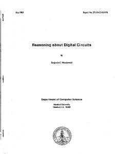
The basic principle for decrementing some counter 22 times is the same one used in Lipton’s proof [Lip76], which we now recall briefly. We will have two chains of counters s and s. We will denote the counters in these chains as sN , sN −1 , . . . , s1 and sN , sN −1 , . . . , s1 N N respectively. If the counter sN has the value 22 , we describe how to decrement it 22 times. i i Further, if the counter si has the value 22 , we describe how to decrement it 22 times. For this, we will use four more chains y, y, z and z. Our description assumes that for each i, the i counters yi and zi have the value 22 (initializing these values will be described later as part i of implementing step (1) in the proof of Theorem 5.4). Decrementing si 22 times is done by nested loops as shown in Figure 3. The outer loop is indexed by yi−1 and the inner loop by i−1 zi−1 . Since both yi−1 and zi−1 have the value 22 , the instruction inside the inner loop i−1 i−1 i (decrementing si ) is executed 22 × 22 = 22 times. To implement these loops, we will need to test when yi−1 and zi−1 become zero. This is done the same way as above, replacing i, i − 1 by i − 1, i − 2 respectively. These two zero tests are done recursively by the same set of transitions. After the recursive zero test, there needs to be a mechanism to determine if the recursive call was made from the inner loop or the outer loop. This mechanism is provided by a chain of counters stack: if the ith counter in the chain stack has the value 1 (respectively 0), then the recursive call was made by the inner (respectively outer) loop. We now give the implementation of instructions that follow the control state named zero in item (3) of page 21 above. In some intermediate configurations when the implementation is executing, the four pointers of the four chains y, z, s and stack will all be pointing to the ith counters of their chains. In this case, we say that the system is at stage i. The N th stage is the last one. We frequently need to move all four pointers to the next stage or previous stage, for which we introduce some macros. The macro Nextstage is short for the sequence of transitions next(y); next(y); . . . ; next(stack); next(stack), which moves all the pointers one stage up. The macro Prevstage similarly moves all the pointers one stage down. The macro transfer(z, s) is intended to transfer the value of the counter in z at current stage to the respective counter in s. The macro consists of the following transitions.


23

i−1

yi−1 = zi−1 = 22 ++ y−− i−1 , yi−1 ++ z−− i−1 , zi−1 ++ s−− i , si

no

zi−1 = 0? yes 2i−1

zi−1 = 2 no

; zi−1 = 0

yi−1 = 0? yes 2i−1

yi−1 = 2

; yi−1 = 0

return i

Figure 3: Control flow of algorithm that decrements si 22 times. : transfer(z, s) : { : subtract: inc(z); dec(z); inc(s); dec(s); /* subtract a count from z and add it to s */ : goto subtract or exit macro /* non-deterministically choose to repeat another step of the count transfer or to exit the macro */

: } The macro transfer(y, s) is similar to the above, with y and y replacing z and z respectively. The macro inc(next(z)) moves the pointer of the chain z one stage up, increments z once and moves the pointer back one stage down: next(z); inc(z); prev(z). The macros inc(next(y)) and inc(next(s)) are similar to inc(next(z)) with y and s replacing z respectively. The macro dec(next(s)) is similarly defined to decrement the next counter in the chain s. The macro stack == 1 tests if the counter in the current stage in the chain stack is greater than 0: dec(stack); inc(stack). Following is the set of transitions at the control state zero in (3) in the proof of Theorem 5.4 above. The listing below is written in the form of a program in a low level programming language for readability. It can be easily translated into a set of transitions of a chain system. There is a control state between every two consecutive instructions below, but only the important ones are given names like “outerloop2”. A line such as “innernonzero2: dec(z); inc(z); goto innerloop2” actually represents the set of transitions {hinnernonzero2, dec(z), qi, hq, inc(z), innerloop2i}. The instruction “q: if first(α)? then {program 1} else {program 2}” represents the set of transitions {hq, first(α)?, q1 i, hq, first(α)?, q2 i}∪

{transitions for program 1 from q1 } ∪ {transitions for program 2 from q2 }.

24


An instruction of the form “q : inc(stack); goto outernonzero2 or outerzero2” represents the set of transitions {hq, inc(stack), outernonzero2i, hq, inc(stack), outerzero2i}. Depending on the non-deterministic choices made at control states that have multiple transitions enabled, there will be several different runs. We prove later that there is one run which has the intended effect and the other runs will never reach the final state. N The action [decrement counters 22 times] in item (3) of page 21 is implemented in Chain system 5.1 by “transfer(counters, s); goto Deczerorep ” in the first line. There is a non-deterministic choice for exiting “transfer(counters, s)”, and we wish to block any run N that exits before incrementing s 22 times. This is done by “goto Deczerorep ”, which forces N the chain system to decrement s 22 times. zero: (next(counters); next(counters))j ; transfer(counters, s); goto Deczerorep zerorep: transfer(counters, s); goto Deczeropass zeropass: (prev(counters); prev(counters))j ; goto q1 Dechaddressi : if first(stack)? then : (dec(s))4 ; (inc(s))4 ; goto DecFinished : else : Prevstage : outerloop2: dec(y); inc(y) /* y is the index for outer loop */ : innerloop2: dec(z); inc(z) /* z is the index for inner loop */ : dec(next(s)); inc(next(s)) : innertest2: goto innernonzero2 or innerzero2 : innernonzero2: dec(z); inc(z); goto innerloop2 /* inner loop not yet complete */ : innerzero2: transfer(z, s); inc(stack); dec(stack); goto Dechaddressi /* inner loop

: : : : :

complete. (i − 1)th counter of stack is set to 1, so the recursive call to Dechaddressi returns to outertest2 */

: outertest2: dec(stack); inc(stack); goto outernonzero2 or outerzero2 : outernonzero2: dec(y); inc(y); goto outerloop2 /* outer loop not yet complete */ : outerzero2: transfer(y, s); goto Dechaddressi /* outer loop complete. (i − 1)th counter of stack is set to 0, so the recursive call to Dechaddressi returns to outerexit2 */

: outerexit2: Nextstage; goto DecFinished : : : : :

fi DecFinished: goto backtrack backtrack: if (last(stack)?) then /* is the pointer at some intermediate stage, which means we just completed a recursive call? */

: if (stack == 1) then goto outertest2 /* ith counter of stack is set to 1, so return to outertest2 */ : else goto outerexit2 /* ith counter of stack is set to 0, so return to outerexit2 */ : else /* pointer is at the last stage, decrementation is complete */ : goto haddressi : fi Chain system 5.1: Decrement j th counter in counters 22

N

times.


25

Suppose, as in the proof of Theorem 5.4, we want to simulate the cj = 0 case of the counter automaton’s transition hq : if cj = 0 goto q1 else cj ← cj − 1 goto q2 i. The N action [increment counters 22 times] in the proof of Theorem 5.4 is implemented above by “transfer(counters, s); goto Deczeropass ” in the second line. If Deczeropass returns successfully, the control can go to q1 as required. The only difference between Deczerorep and Deczeropass is the return address zerorep and zeropass. A generic Dechaddressi is shown above, which implements the algorithm shown in Figure 3. Formally, every instruction label (such as outerloop2, innerloop2 etc.) should also be parameterized with haddressi, but these have been ommitted for the sake of readability. The case “if first(stack)?” implements the base case i = 1. If i > 1, the else branch is taken, where the first instruction is to move all pointers one stage down, so that they now point to yi−1 and zi−1 as required by the algorithm of Figure 3. The loop between outerloop2 and outerzero2 implements the outer loop of Figure 3 and the loop between innerloop2 and innerzero2 implements the inner loop of Figure 3. The non-deterministic choice in innertest2 decides whether to continue the inner loop or to exit. The macro transfer(z, s) at the beginning of innerzero2 will i−1 reset the (i − 1)th counter of z back to 22 , at the same time setting (i − 1)th counter of s i−1 i−1 to 22 . So the run that behaves as expected increments zi−1 exactly 22 times. All other runs are blocked by the recursive call to Dechaddressi at the end of innerzero2. The purpose of inc(stack); dec(stack); in the middle of innerzero2 is to ensure that the recursive call to Dechaddressi returns to the correct state. After similar tests in outerzero2, “Nextstage” at the beginning of outerexit2 moves all the pointers back to stage i. Then in backtrack, the correct return state is figured out. Exactly how this is done will be clear in the proof of the following lemma, where we construct runs of the chain system by induction on stage. Lemma 5.5. In the state zero in the listing above, if the j th counter in the chain counters has the value 0, there is a run that reaches the state q1 without causing any changes. Any run from the state zero will be blocked if the j th counter in the chain counters has a value other than 0. Proof. We first prove the existence of a run reaching q1 when the j th counter in the chain N counters has the value 0. The j th counter in the chain counters will have the value 22 . N Our run executes transfer(counters, s) to set countersj and sN to 22 and set sN and countersj to 0. With these values in the counters, we will prove next that there is run from N Deczerorep to zerorep that sets sN to 0 and sN to 22 . From zerorep, our run continues to execute transfer(counters, s) to set countersj and sN to 0 and set countersj and sN N to 22 . Then there is again a run from Deczeropass to zeropass which sets sN to 0 and N sets sN to 22 . From zeropass, our run moves the pointers on the chains counters and counters back to the first position and goes to state q1 . N Now suppose that in the state Dechaddressi , sN is set to 22 , sN is set to 0 and the pointer in the chain stack is at the last position, as mentioned in the previous paragraph. N We will prove that there is a run that reaches haddressi, setting sN to 0 and sN to 22 . We will in fact prove the following claim by induction on i. i Claim: Suppose that in the state Dechaddressi , si is set to 22 , si is set to 0 and the pointers in the chains stack, s, y, z are at position i. There is a run ρi that reaches DecFinished, i setting si to 0 and si to 22 , with the pointers in the same position. When we first call Deczerorep or Deczeropass , the pointers in the chains stack, s, y, z are at the last position (N ). Hence, when the run ρN given by the above claim reaches

26


DecFinished, it can continue to the state backtrack and then to zerorep or zeropass respectively. Base case of the claim: i = 1. The run ρ1 is as follows: if first(stack)? then (dec(s))4 ; (inc(s))4 ; goto DecFinished . Induction step of the claim:. The run ρi+1 is as follows. : Prevstage : outerloop2: dec(y); inc(y) : innerloop2: dec(z); inc(z) : dec(next(s)); inc(next(s)) i : innertest2: goto innernonzero2 22 − 1 times, then goto innerzero2 : innernonzero2: dec(z); inc(z); goto innerloop2 : innerzero2: transfer(z, s); inc(stack); dec(stack); goto Dechaddressi /* Follow ρi here. Since we set stacki to 1, we can return to outertest2 at the end of ρi to continue our ρi+1 */ i

: outertest2: dec(stack); inc(stack); goto outernonzero2 22 − 1 times, then goto outerzero2 : outernonzero2: dec(y); inc(y); goto outerloop2 : outerzero2: transfer(y, s); goto Dechaddressi /* Follow ρi here. Since now stacki is 0, we can return to outerexit2 at the end of ρi to continue our ρi+1 */

: outerexit2: Nextstage; goto DecFinished This completes the induction step and the proof of the claim. Finally, we will prove that any run from zero will be blocked if the j th counter in the chain counters has a value other than 0. Indeed, the j th counter in the chain counters has N a value less than 22 when the state is Deczerorep . Hence no run can execute innerloop2 N −1 and outerloop2 22 times. Hence, any run will either get blocked when the pointer in N −1 the chain s is still at position N , or it will go to state Dechaddressi with sN −1 less than 22 . In the latter case, we can argue in the same way to conclude that any run is blocked either when the pointer in the chain s is still at N − 1 or it will go to state Dechaddressi with sN −2 N −2 less than 22 and so on. Any run is blocked at some stage between N and 1. Next, we explain the implementation of step (1) in the proof of Theorem 5.4. We show how to get counters to their required initial values (at the beginning of the runs all the values are equal to zero). We briefly recall the required initial values: (1) each counter c has value zero, (2) for every i ∈ [1, N ], yi , zi and si are equal to zero, (3) for every i ∈ [1, N ], stacki is equal to zero and stacki is equal to one, N (4) each complement counter c has value 22 , i (5) for every i ∈ [1, N ], yi , zi and si have the value 22 . The initialization for the points (1)–(3) is easy to perform and below we focus on the initialization for the point (5). Initialization of the complement counter in point (4) will be dealt with later by simply adjusting what is done below. To help achieve these initial values for 5), we have another chain init, with N counters. We follow the convention that if at stage i, the counter in the chain init has value 1, then all the counters in all the chains at stage i or below have been properly initialized. By convention, the condition last(init)? is true if the pointer in the chain init is at stage N . The macros Nextstage and Prevstage moves the pointers of the chain init, in addition to all the other chains.


27

We now give the code used to initialize y, z, s and stack to the required values, assuming that all counters are initially set to 0 and all the pointers in all the chains are pointing to stage 0. The counters y0 , z0 , s0 and stack0 are initialized directly. For the counters at higher stages, we again use nested loops similar to those shown in Figure 3, assuming that counters at lower stages have been initialized. These nested loops are implemented between innerinit–innerzero1 and outerinit–outerzero1. The zero tests involved in terminating these loops are performed by the same decrementing algorithm, assuming that counters at lower stages are already initialized. This will introduce some complications while backtracking from the decrementing algorithm — we have to figure out whether the call to Dec was from innerzero1 or outerzero1, or from within Dec itself from a recursive call. To handle this, the “backtrack” part of the code below has been updated to check if (next(init) == 1): if so, we are inside some recursive call to Dec. Otherwise, the call to Dec was from one of the loops initializing a higher level. : begininit: (inc(y))4 ; (inc(z))4 ; (inc(s))4 ; inc(init); inc(stack) : initialize: If last(init)? goto beginsim else goto outerinit : outerinit: dec(y); inc(y) /* y is the index for outer loop */ : innerinit: dec(z); inc(z) /* z is the index for inner loop */ : INC: inc(next(y)); inc(next(z)); inc(next(s)) : innertest1: goto innernonzero1 or innerzero1 : innernonzero1: dec(z); inc(z); goto innerinit /* inner loop not yet complete */ : innerzero1: transfer(z, s); inc(stack); dec(stack); goto Dec /* inner loop complete. (next(init) == 0) and (stack == 1), so Dec returns to outertest1 */

: outertest1: dec(stack); inc(stack); goto outernonzero1 or outerzero1 : outernonzero1: dec(y); inc(y); goto outerinit /* outer loop not yet complete */ : outerzero1: transfer(y, s); goto Dec /* outer loop complete. (next(init) == 0) and (stack == 0), so Dec returns to outerexit1 */

: outerexit1: Nextstage; inc(init); inc(stack); goto initialise : beginsim: start simulating the counter machine (see part of the proof of Theorem 5.4 related to the simulation) : : Dec: : if first(init)? then : (dec(s))4 ; (inc(s))4 ; goto DecFinished : else : Prevstage : outerloop2: dec(y); inc(y) /* y is the index for outer loop */ : innerloop2: dec(z); inc(z) /* z is the index for inner loop */ : dec(next(s)); inc(next(s)) : innertest2: goto innernonzero2 or innerzero2 : innernonzero2: dec(z); inc(z); goto innerloop2 /* inner loop not yet complete */ : innerzero2: transfer(z, s); inc(stack); dec(stack); goto Dec /* inner loop complete. (next(init) == 1) and (stack == 1), so Dec returns to outertest2 */

: outertest2: dec(stack); inc(stack); goto outernonzero2 or outerzero2 : outernonzero2: dec(y); inc(y); goto outerloop2 /* outer loop not yet complete */ : outerzero2: transfer(y, s); goto Dec /* outer loop complete. (next(init) == 1) and (stack == 0), so Dec returns to outerexit2 */

: outerexit2: Nextstage; goto DecFinished

28


fi DecFinished: goto backtrack backtrack: if (next(init) == 1) then /* we are not at the end of recursion */ : if (stack == 1) then goto outertest2 : else goto outerexit2 : else /* we are at the end of recursion */ : if (stack == 1) then goto outertest1 : else goto outerexit1 : fi The ideas involved in the above listing are similar to the ones in the code decrementing N countersj 22 times. : : : :

Lemma 5.6. Suppose the control state is begininit, all the pointers in all the chains are at stage 1 and all the counters at all stages have the value 0. For any i between 1 and N , there is a run ρ0i ending at initialise, such that the pointer is at stage i in all the chains and all the counters at or below stage i have been initialised. If a run starts from begininit as above, it will not reach beginsim unless all the counters have been properly initialized. Proof. By induction on i. For the base case i = 1, ρ01 is the run that executes the instructions immediately after begininit and ends at initialise. Now we assume the lemma is true up to i and prove it for i + 1. By induction hypothesis, there is a run ρ0i ending at initialise, with all the pointers in all the chains at stage i and all the counters at or below stage i initialised. The run ρ0i+1 is obtained by appending the following sequence to ρ0i . It uses the runs ρi constructed in the proof of Lemma 5.5. : initialise: If last(init)? goto beginsim else goto outerinit /* pointer in chain init is at i 6= N ; go to outerinit */

: outerinit: dec(y); inc(y) : innerinit: dec(z); inc(z) : INC: inc(next(y)); inc(next(z)); inc(next(s)) i : innertest1: goto innernonzero1 22 − 1 times then goto innerzero1 : innernonzero1: dec(z); inc(z); goto innerinit /* inner loop not yet complete */ : innerzero1: transfer(z, s); inc(stack); dec(stack); goto Dec /* follow ρi here;

since

(next(init) == 0) and stack == 1, we can retrun to outertest1 to continue our ρ0i+1 */ i outertest1: dec(stack); inc(stack); goto outernonzero1 22 − 1 times then

goto outerzero1 : outernonzero1: dec(y); inc(y); goto outerinit : outerzero1: transfer(y, s); goto Dec /* follow ρi here; since (next(init) == 0) and stack == 0, we :

can retrun to outerexit1 to continue our ρ0i+1 */

: outerexit1: Nextstage; inc(init); inc(stack); goto initialise This completes the induction step, proving the existence of a run ending at initialize as required. Finally we argue that any run from begininit that does not initialize all the counters properly will get stuck. Indeed, the only way out of the initialization code is to go to beginsim, which is only reachable via initialize. From initialize, we can go to beginsim only when the pointers are at stage N . We finish the argument by showing that any run that visits initialize for the first time with pointers at stage i would have initialized all


29

counters at or below stage i. The only way to go to initialize with pointers at stage i is via begininit (for i = 1) or via outerexit1 (for i > 1). It is clear in the case of i = 1 that the counters at stage 1 are properly initialized. In the case of i > 1, the only way to reach outerexit1 is via Dec. In this case, all runs are forced to iterate the loops at outerinit and innerinit the correct number of times as we have seen in the proof of Lemma 5.5, which will again force all the counters at or below stage i to be properly initialized. To complete the proof of Theorem 5.4, we finally show how to initialize the first D ≤ n counters from counters and counters that correspond to the counters of the original counter automaton (point (4) of the initialization values listed after Lemma 5.5). This is achieved by replacing the code for INC from the code for the initialization phase by the following one: : INC: inc(next(y)); inc(next(z)); inc(next(s)) : next(init) if last(init)? then : inc(counters) : (next(counters);inc(counters))D−1 : (prev(counters))D−1 prev(init) This finishes the proof of Theorem 5.4. 5.3. Reasoning About Chain Systems with LRV. Given a chain system A of level 1, we construct a polynomial-size formula in LRV that is satisfiable iff A has a gainy accepting run. Hence, we get a 2expspace lower bound for SAT(LRV). The main idea is to encode runs of chain systems with LRV formulas that access the counters using binary encoding, so that the formulas can handle exponentially many counters. Lemma 5.7. There is a polynomial-time reduction from Gainy(1) into SAT(LRV(X, F)). Proof. Let A = hQ, f, 1, Q0 , QF , δi be a chain system of level 1 with f : [1, n] → N, having thus n chains of counters, of respective size 2f (1) , . . . , 2f (n) . We encode a word ρ ∈ δ ∗ that represents an accepting run. For this, we use the alphabet δ of transitions. Note that we can easily simulate the labels δ = {t1 , . . . , tm } with the variables t0 , . . . , tm , where a node has an encoding of the label ti iff the formula def hti i = t0 ≈ ti holds true. We build a LRV formula ϕ so that there is an accepting gainy run ρ ∈ δ ∗ of A if, and only if, there is a model σ so that σ |= ϕ and σ encodes the run ρ. The following are standard counter-blind conditions to check. (a) Every position satisfies hti for some unique t ∈ δ. (b) The first position satisfies h(q0 , instr, q)i for some q0 ∈ Q0 , instr ∈ I, q ∈ Q. (c) The last position satisfies h(q, instr, q 0 )i for some q ∈ Q, instr ∈ I, q 0 ∈ QF . (d) There are no two consecutive positions i and i + 1 satisfying h(q, u, q 0 )i and h(p, u0 , p0 )i respectively, with q 0 6= p.

We use a variable x, and variables xαinc , xαdec , xαi for every chain α and for every i ∈ [1, f (α)]. Let us fix the bijections χα : [0, 2f (α) − 1] → 2[1,f (α)] for every α ∈ [1, n], that assign to each number m the set of 1-bit positions of the representation of m in base 2. We say that a position i in a run is α-incrementing [resp. α-decrementing] if it satisfies h(q, u, q 0 )i for some q, q 0 ∈ Q and u = inc(α) [resp. u = dec(α)].

30


In the context of a model σ with the properties ((a))–((d)), we say that a counter position i in a run operates on the α-counter c, if χα (c) = Xi , where Xi = {b ∈ [1, f (α)] | σ(i)(x) = σ(i)(xαb )}.

(5.2)

Note that thus 0 ≤ c < 2f (α) . For every chain α, let us consider the following properties: (1) Any two positions of σ have different values of xαinc [resp. of xαdec ]. (2) For every position i of σ operating on an α-counter c containing an instruction ‘first(α)?’ [resp. ‘first(α)?’, ‘last(α)?’, ‘last(α)?’], we have c = 0 [resp. c = 6 0, c = 2f (α) − 1, c 6= 2f (α) − 1]. (3) For every position i of σ operating on an α-counter c, • if the position contains an instruction ‘next(α)’ [resp. ‘prev(α)’], then the next position i + 1 operates on the α-counter c + 1 [resp. c − 1], • otherwise, the position i + 1 operates on the α-counter c. (4) For every α-incrementing position i of σ operating on an α-counter c there is a future α-decrementing position j > i operating on the same α-counter c, such that σ(i)(xαinc ) = σ(j)(xαdec ). Claim 5.8. There is a model satisfying the conditions above if, and only if, A has a gainy and accepting run. Proof. (Only if ) Suppose we have a model σ that verifies all the properties above. Since by (1), all the positions have different data values for xαdec , it then follows that the position j to which property (4) makes reference is unique. Since, also by (1), all the positions have different data values for xαinc , we have that the α-decrement corresponds to at most one α-increment position in condition (4). Moreover, it is an α-decrement of the same counter, that is, Xi = Xj (cf. (5.2)). For these reasons, for every α-increment there is a future α-decrement of the same counter which corresponds in a unique way to that increment. More precisely, for every chain α, the function γσα : {0 ≤ i < |σ| : i is α-incrementing} → {0 ≤ i < |σ| : i is α-decrementing}

where γσα (i) = j iff σ(i)(xαinc ) = σ(j)(xαdec ) is well-defined and injective, and for every γσα (i) = j we have that j > i and Xi = Xj . Consider ρ ∈ δ ∗ as having the same length as σ and such that ρ(i) = (q, instr, q 0 ) whenever σ, i |= h(q, instr, q 0 )i. From conditions (2) and (3), it follows that the counter cαi corresponding to position i from ρ, is equal to χ−1 (Xi ). Therefore, the functions {γσα }α∈[1,n] witness the fact that ρ is a gainy and accepting run of A. (If ) Let us now focus on the converse, by exhibiting a model satisfying the above properties, assuming that A has an accepting gainy run ρ ∈ δ ∗ . We therefore have, for every α ∈ [1, n], an injective function γ α : {i | ρ(i) is α-incrementing} → {i | ρ(i) is α-decrementing}

where for every γ α (i) = j we have that j > i and cαi = cαj . We build a model σ of the same length of ρ, and we now describe its data values. Let us fix two distinct data values d, e. For any position i, we have σ(i)(t0 ) = d; and σ(i)(tj ) = d if the ith transition in ρ is tj and σ(i)(tj ) = e otherwise. In this way we make sure that the properties ((a))–((d)) hold.


31

We use distinct data values d0 , . . . , d|σ|−1 and d00 , . . . , d0|σ|−1 (all different from d, e). We define the data values of the remaining variables for any position i: • For every α, σ(i)(xαinc ) = di . • For every α, – if i is α-decrementing, we define σ(i)(xαdec ) = σ(i0 )(xαinc ) where i0 = (γ α )−1 (i); if such (γ α )−1 (i) does not exist, then σ(i)(xαdec ) = d0i ; – otherwise, if i is not α-decrementing, σ(i)(xαdec ) = d0i . • σ(i)(x) = d. • For every α, σ(i)(xαl ) = σ(i)(x) = d if l ∈ χ(cαi ), otherwise σ(i)(xαl ) = e. Observe that these last two items ensure that the properties (2) and (3) hold. By definition, every position of σ has a different data value for xαinc . Let us show that the same holds for xαdec . Note that at any position i, xαdec has: the data value of σ(i0 )(xαinc ) = di0 for some i0 < i; or the data value d0i . If there were two positions i < j with σ(i)(xαdec ) = σ(j)(xαdec ) it would then be because: (i) d0i = d0j ; (ii) di0 = d0j for some i0 < i; (iii) d0i = dj 0 for some j 0 < j; or (iv) di0 = dj 0 for some i0 < i, j 0 < j. It is evident that none of (i), (ii), (iii) can hold since all d0 , . . . , d|σ|−1 , d00 , . . . , d0|σ|−1 are distinct. For this reason, if (iv) holds, it means that i0 = j 0 , and hence that (γ α )−1 (i) = (γ α )−1 (j), implying that γ α is not injective, which is a contradiction. Hence, all the positions have different data values for xαdec . Therefore, σ has the property (1). To show that σ has property (4), let i be a α-incrementing position of σ, remember that σ(i)(xαinc ) = di . Note that position γ α (i) = j must be α-decrementing on the same counter. By definition of the value of xαdec , we have that σ(j)(xαdec ) must be equal to σ((γ α (j))−1 )(xαinc ) = σ(i)(xαinc ) = di . Thus, property (4) holds. We complete the reduction by showing that all the properties expressed before can be efficiently encoded in our logic. Claim 5.9. Properties ((a))–((d)) and (1)–(4) can be expressed by formulas of LRV, that can be constructed in polynomial time in the size of A. Proof. Along the proof, we use the following formulas, for any α ∈ [1, n] and for any i ∈ [1, f (α)], def bit αi = x ≈ xαi , where bit α1 represents the most significant bit. Now, we show how to code each of the properties. • Properties ((a))–((d)) are easy to express in LRV and present no complications. • For expressing (1), we force xαinc and xαdec to have a different data value for every position of the model with the formula ¬F xαinc ≈ h>?ixαinc ∧ ¬F xαdec ≈ h>?ixαdec .

• Property (2) is straightforward to express in LRV. • We express property (3) by first determining which is the bit i that must be flipped for the increment of the counter pointer of the chain α (the least significant bit is the f (α)th one). ^ def flipαi = ¬bit αi ∧ bit αj j>i

32


Then by making sure that all the bits before i are preserved. ^ def copyαi = (bit αj ⇔ X(bit αj )) ji

And finally by swapping the bit i. def

swapαi = X bit αi Hence, the property to check is, for every α ∈ [1, n], ^ ^ h(q, next(α), q 0 )i ⇒ flipαi ⇒ copyαi ∧ zeroαi ∧ swapαi . (q,next(α),q 0 )∈δ

i∈[1,n]

The formula expressing the property for decrements of counter pointers (prev(α)) is analogous. • Finally, we express property (4) by testing, for every α-incrementing position, _ xαinc ≈ hα-dec?ixαdec where α-dec = h(q, dec(α), q 0 )i (q,dec(α),q 0 )∈δ

and for every i ∈ [1, f (α)],

bit αi ⇒ xαinc ≈ hbit αi ?ixαdec ∧ ¬bit αi ⇒ xαinc ≈ h¬bit αi ?ixαdec .

If the α-increment has some data value d at variable xαinc , there must be only one future position j where xαdec carries the data value d —since every xαdec has a different value, by (1). For this reason, both positions (the α-increment and the α-decrement) operate on the same counter, and thus the formula faithfully expresses property (4). As a corollary of Claims 5.8 and 5.9 we obtain a polynomial-time reduction from Gainy(1) into the satisfiability problem for LRV(X, F). 6. A Robust Equivalence We have seen that the satisfiability problem for LRV is equivalent to the control state reachability problem in an exponentially larger VASS. In this section we evaluate how robust is this result with LRV variants or fragments. We consider infinite data words (instead of finite data words), finite sets of MSO-definable temporal operators (instead of X, X−1 , S, U) and also repetitions of pairs of values (instead of repetitions of single values). 6.1. Infinite Words with Multiple Data. So far, we have considered only finite words with multiple data. It is also natural to consider the variant with infinite words but it is known that this may lead to undecidability: for instance, freeze LTL with a single register is decidable over finite data words whereas it is undecidable over infinite data words [DL09]. By contrast, FO2 over finite data words or over infinite data words is decidable [BMS+ 06]. Let SATω ( ) be the variant of the satisfiability problem SAT( ) in which infinite models of length ω are taken into account instead of finite ones. The satisfaction relation for LRV, PLRV, LRV> , etc. on ω-models is defined accordingly.


33

Proposition 6.1. (I): SATω (PLRV) is decidable. (II): SATω (LRV) is 2expspace-complete. Proof. (I) The developments of Section 4.1 apply to the infinite case, and since SATω (PLRV> ) is shown decidable in [DDG12], we get decidability of SATω (PLRV). (II) First, note that SATω (LRV) is 2expspace-hard. Indeed, there is a simple logarithmicspace reduction from SAT(LRV) into SATω (LRV), which can be performed as for standard LTL. Indeed, it is sufficient to introduce two new variables xnew and ynew , to state that xnew ≈ ynew is true at a finite prefix of the model (herein xnew ≈ ynew plays the role of a new propositional variable) and to relativize all the temporal operators and obligations to positions on which xnew ≈ ynew holds true. Concerning the complexity upper bound, from Section 4.1, we can conclude that there is a polynomial-time reduction from SATω (LRV) into SATω (LRV> ). The satisfiability problem SATω (LRV> ) is shown decidable in [DDG12] and we can adapt developments from Section 4.2 to get also a 2expspace upper bound for SATω (LRV> ). This is the purpose of the rest of the proof. By analyzing the constructions from [DDG12, Section 7], one can show that φ of LRV> built over the variables {x1 , . . . , xk } is ω-satisfiable iff there are Z ⊆ P + ({x1 , . . . , xk }), a VASS AZ φ = hQ, Z, δi along with sets Q0 , Qf ⊆ Q of initial and final states respectively and a B¨ uchi automaton B Z such that: ∗ (1) AZ − hqf , 0i in AZ φ is the restriction of Aφ defined in Section 4.2 and hq0 , 0i → φ for some q0 ∈ Q0 and qf ∈ Qf . (2) B Z accepts a non-empty language. ∗

By arguments similar to those from Section 4.2, existence of a run hq0 , 0i → − hqf , 0i can be checked in 2expspace. Observe that in the construction in [DDG12, Section 7], counters in P + ({x1 , . . . , xk }) \ Z are also updated in AZ φ (providing the VASS Aφ ) but one can show that this is not needed because of optional decrement condition and because B Z is precisely designed to take care of the future obligations in the infinite related to the counters in P + ({x1 , . . . , xk }) \ Z. B Z can be built in exponential time and it is of exponential size in the size of φ. Hence, non-emptiness of B Z can be checked in expspace. Finally, the number of possible subsets Z is only at most double exponential in the size of φ, which allows to get a nondeterministic algorithm in 2expspace and provides a 2expspace upper bound by Savitch’s Theorem [Sav70].

6.2. Adding MSO-Definable Temporal Operators. It is standard to extend the lineartime temporal logic LTL with MSO-definable temporal operators (see e.g. [Wol83, GK03]), and the same can be done with LRV. For this, one considers MSO formulas over a linear order in > x ≈ hφ?iy. Let LRVk [resp. LRV> k , PLRVk ] be the restriction to formulas with at most k variables. In [DDG12, Theorem 5], it is shown that SAT(LRV> 1 ) is pspace-complete by establishing a reduction into the reachability problem for VASS when counter values are linearly bounded. Below, we generalize this result for any k ≥ 1 by using the proof of Theorem 4.12 and the fact that the control state reachability problem for VASS with at most k counters (where k is a constant) is in pspace.

36


x1

2

3

2

σ : x2

1

2

7

x3

1

6

3

segment 1

σϕ : x

5

2

5

1

γ2

5

segment 2 1

5

5

3

5

2

5

segment 3 6

5

γ3

5

2

5

7

5

3

5

γ1

Figure 4: Example of the reduction from SAT(LRV> ) into SAT(LRV1 ), for k = 3, N = 3 and d = 5 Proposition 6.4. For every k ≥ 1, SAT(LRV> k ) is pspace-complete. Proof. pspace-hardness is due to the fact that LTL with a single propositional variable is pspace-hard [DS02], which can be easily simulated with the atomic formula x ≈ Xx. Let k ≥ 1 be some fixed value and φ ∈ LRV> k . In the proof of Theorem 4.12, we have seen that there exist a VASS Adec = hQ, C, δi and Q0 , Qf ⊆ Q such that φ is satisfiable iff there are ∗ qf ∈ Qf and q0 ∈ Q0 such that hqf , 0i → − hq0 , vi for some counter valuation v. Note that the number of counters in Adec is bounded by 2k , card(Q) is exponential in |φ| and the maximal value for an update in a transition of Adec is k. Moreover, deciding whether a state in Q belongs to Q0 [resp. Qf ] can be checked in polynomial space in |φ| and δ can be decided in polynomial space too. By using [Rac78] (see also [DJLL09]), we can easily conclude that ∗ ∗ hqf , 0i → − hq0 , vi for some counter valuation v iff hqf , 0i → − hq0 , v0 i for some v0 such that the length of the run is bounded by p(|Adec | + max(Adec ))f(k) where p(·) is a polynomial, f is a map of double exponential growth and max(Adec ) denotes the maximal absolute value in an update (bounded by k presently). Since k is fixed, the length of the run is at most exponential in |φ|. Consequently, the following polynomial-space nondeterministic algorithm allows to check whether φ is satisfiable. Guess qf ∈ Qf , q0 ∈ Q0 and guess on-the-fly a run of length at most p(|Adec | + max(Adec ))f(k) from hqf , 0i to some hq0 , v0 i. Counter valuations can be represented in polynomial space too. By Savitch’s Theorem [Sav70], we conclude that the satisfiability problem for LRV> k is in pspace. This does not imply that LRVk is in pspace, since the reduction from LRV into LRV> in Section 4.1 introduces new variables. In fact, it introduces a number of variables that depends on the size of the formula. It turns out that this is unavoidable, and that its satisfiability problem is 2expspace-hard, by the following reduction. Lemma 6.5. There is a polynomial-time reduction from SAT(LRV> ) into SAT(LRV1 ) [resp. SAT(PLRV> ) and SAT(PLRV1 )]. Proof. The idea of the coding is the following. Suppose we have a formula ϕ ∈ LRV> using k variables x1 , . . . , xk so that σ |= ϕ. We will encode σ in a model σϕ that encodes in only one variable, say x the whole model of σ restricted to x1 , . . . , xk . To this end, σϕ is divided into N segments s1 · · · sN of equal length, where N = |σ|. A special fresh data value is used as a special constant. Suppose that d is a data value that is not in σ. Then, each segment si has length k 0 = 2k + 1, and is defined as the data values “d d1 d d2 . . . d dk d”, where dj = σ(i)(xj ). Figure 4 contains an example for k = 3 and N = 3. In fact, we can force that the model has this shape with LRV1 . Note that with this coding, we can tell that we are between two segments if there are two consecutive equal data values. In fact, we are at a position corresponding to xi (for


37

i ∈ [1, k]) inside a segment if we are standing at the 2i-th element of a segment, and we can test this with the formula 0

0

0

0

γi = Xk −2i x ≈ Xk −2i+1 x ∨ (Xk −2i > ∧ ¬Xk −2i+1 >).

Using these formulas γi , we can translate any test xi ≈ h>?ixj into a formula that (1) moves to the position 2i of the segment (the one corresponding to the xi data value), (2) tests x ≈ hγj ?ix. We can do this similarly with all formulas. Let us now explain in more detail how to do the translation, and why it works. Consider the following property of a given position i multiple of k 0 of a model σϕ : • for every j ∈ [0, k 0 − 1], σϕ (i + j)(x) = σϕ (i)(x) if, and only if, j is even, and • either i + k 0 ≥ |σϕ | or σϕ (i + k 0 ) = σϕ (i). This property can be easily expressed with a formula ^ ^ 0 0 segment-k 0 = x ≈ Xj x ∧ x 6≈ Xj x ∧ (¬Xk > ∨ x ≈ Xk x). 0≤j≤k0 −1, j is even

0≤j≤k0 −1, j is odd

Note that this formula tests that we are standing at the beginning of a segment in particular. It is now straightforward to produce a LRV1 formula that tests • σϕ , 0 |= segment-k 0 • for every position i so that σϕ (i)(x) = σϕ (i + 1)(x), we have σ, i + 1 |= segment-k 0 . Let us call many-segments the formula expressing such a property. Note that the property implies that σϕ is a succession of segments, as the one of Figure 4. We give now the translation of a formula ϕ of LRV> with k variables into a formula ϕ0 of LRV1 with 1 variable. k0 times

z }| { tr(Xψ) = X · · · X tr(ψ) k0 times

}| { z −1 −1 −1 tr(X ψ) = X · · · X tr(ψ)

tr(Fψ) = F(segment-k 0 ∧ tr(ψ))

tr(ψUγ) = (segment-k 0 ⇒ tr(ψ) U (segment-k 0 ∧ tr(γ)) tr(ψSγ) = (segment-k 0 ⇒ tr(ψ) S (segment-k 0 ∧ tr(γ)) 0

tr(xi ≈ X` xj ) = X2i−1 x ≈ X`·k +2j−1 x

(and similarly for 6≈)

Now we have to translate xi ≈ h>?ixj . This would be translated in our encoding by saying that the i-th position of the current segment is equal to the j-th position of a future segment. Note that the following formula ξi,j = X2i−1 (x ≈ hγj ?ix)

does not exactly encode this property. For example, consider that we would like to test x2 ≈ h>?ix3 at the first element of the model σϕ depicted in Figure 4. Although ξ2,3 holds, the property is not true, there is no future segment with the data value 1 in the position encoding x3 . In fact, the formula ξ encodes correctly the property only when xi 6≈ xj .

38


However, this is not a problem since when xi ≈ xj the formula xi ≈ h>?ixj is equivalent to xj ≈ h>?ixj . We can then translate the formula as follows. tr(xi ≈ h>?ixj ) = (tr(xi ≈ xj ) ∧ ξj,j ) ∨ (tr(xi 6≈ xj ) ∧ ξi,j )

Recall that xi 6≈ h>?ixj is not translated since such formulae can be eliminated. We then define ϕ0 = many-segments ∧ tr(ϕ). Claim 6.6. ϕ is satisfiable if, and only if, ϕ0 is satisfiable.

Proof. In fact, if σ |= ϕ, then by the discussion above, σϕ |= ϕ0 . If, on the other hand, σ 0 |= ϕ0 for some σ 0 , then since σ 0 |= many-segments it has to be a succession of segments of size 2k + 1, and we can recover a model σ of size |σ 0 |/2k + 1 where σ(i)(xj ) is the data value of the 2j-th position of the i-th segment of σ 0 . In this model, we have that σ |= ϕ. This coding can also be extended with past obligations in a straightforward way, −1 −1 tr(xi ≈ hφ?i−1 xj ) = (tr(xi ≈ xj ) ∧ ξj,j ) ∨ (tr(xi 6≈ xj ) ∧ ξi,j ) −1 ξi,j

2i−1

= X

−1

(x ≈ hγj ?i

where

x).

Therefore, there is also a reduction from PLRV> into PLRV1 . Corollary 6.7. For all k ≥ 1, SAT(LRVk ) is 2expspace-complete. Corollary 6.8. For all k ≥ 1, SAT(PLRVk ) is as hard as Reach(VASS). 6.5. The Power of Pairs of Repeating Values. Let us consider the last variant of LRV in which the repetition of tuples of values is possible. Such an extension amounts to introducing additional variables in a first-order setting. This may lead to undecidability since 3 variables are enough for undecidability, see e.g. [BDM+ 11]. However, LRV makes a restricted use of variables, leading to 2expspace-completeness. There might be hope that LRV augmented with repetitions of pairs of values have a reasonable computational cost. Consider an extension to LRV with atomic formulas of the form (x1 , . . . , xk ) ≈ hφ?i(y1 , . . . , yk ) where x1 , . . . , xk , y1 , . . . , yk ∈ VAR. This extends x ≈ hϕ?iy by testing whether the vector of data values from the variables (x1 , . . . , xk ) of the current position coincides with that of (y1 , . . . , yk ) in a future position. The semantics are extended accordingly: σ, i |= (x1 , . . . , xk ) ≈ hϕ?i(y1 , . . . , yk ) iff there exists j such that i < j < |σ|, σ, j |= ϕ, and σ(i)(xl ) = σ(j)(yl ) for every l ∈ [1, k]. We call this extension LRVvec . Unfortunately, we can show that SAT(LRVvec ) is undecidable, even when only tuples of dimension 2 are allowed. This is proved by reduction from a variant of Post’s Correspondence Problem (PCP), see below. In order to code solutions of PCP instances, we adapt a proof technique used in [BDM+ 11] for first-order logic with two variables and two equivalence relations on words. However, our proof uses only future modalities (unlike the proof of [BDM+ 11, Proposition 27]) and no past obligations (unlike the proof of [KSZ10, Theorem 4]). To prove this result, we work with a variant of the PCP problem in which solutions ui1 · · · uin = vi1 · · · vin have to satisfy |ui1 · · · uij | ≤ |vi1 · · · vij | for every j. Theorem 6.9. SAT(LRVvec (X, U)) is undecidable. Let us introduce the problem below as a variant of PCP:


39

Problem: Modified Directed Post’s Correspondence Problem (MPCPdir ) Input: A finite alphabet Σ, n ∈ N, u1 , . . . , un , v1 , . . . , vn ∈ Σ+ , |u1 |, |u2 | ≤ 2 and |v1 |, |v2 | ≥ 3. Question: Are there indices 1 ≤ i1 , . . . , im ≤ n so that ui1 · · · uim = vi1 · · · vim , i1 ∈ {1, 2}, |ui1 · · · uim | is even and for every |ui1 | < j < |ui1 · · · uim |, if the j th position of vi1 · · · vim occurs in vik for some k, then the j th position of ui1 · · · uim occurs in uik0 for some k 0 > k? Lemma 6.10. The MPCPdir problem is undecidable. This is a corollary of the undecidability proof for PCP as done in [HMU01]. By reducing MPCPdir to satisfiability for LRVvec , we get undecidability. Proof. In [HMU01], the halting problem for Turing machines is first reduced to a variation of PCP called modified PCP. In modified PCP, a requirement is that the solution should begin with the pair u1 , v1 (this requirement can be easily eliminated by encoding it into the standard PCP, but here we find it convenient to work in the presence of a generalisation of this requirement). To ensure that there is a solution of even length whenever there is a solution, we let u2 = $u1 and v2 = $v1 , where $ is a new symbol. Now u1 ui2 · · · uim = v1 vi2 · · · vim is a solution iff u2 ui2 · · · uim = v2 vi2 · · · vim is a solution. In modified PCP, |u1 | = 1 and |v1 | ≥ 3. Hence, |u2 | = 2 and |v2 | ≥ 3. The resulting set of strings u1 , . . . , un , v1 , . . . , vn make up our instance of MPCPdir . In the encoding of the halting problem from the cited work, |ui | ≤ 2 for any i between 1 and n (this continues to hold even after we add $ to the first pair as above). A close examination of the proof in the cited work reveals that if the modified PCP instance u1 , . . . , un , v1 , . . . , vn ∈ Σ∗ has a solution ui1 · · · uim = vi1 · · · vim , then for every |ui1 | < j < |ui1 · · · uim |, if the j th position of vi1 · · · vim occurs in vik for some k, then the j th position of ui1 · · · uim occurs in uik0 for some k 0 > k (we call this the directedness property). In short, the reason for this is that for any k ∈ N, if vi1 · · · vik encodes the first ` + 1 consecutive configurations of a Turing machine, then ui1 · · · uik encodes the first ` configurations. Hence, for any letter in vik+1 (which starts encoding (` + 2)th configuration), the corresponding letter cannot occur in ui1 · · · uik +1 (unless the single string uik+1 encodes the entire (` + 1)st configuration and starts encoding (` + 2)th configuration; this however is not possible since there are at most 3 letters in uik+1 and encoding a configuration requires at least 4 letters). After the last configuration has been encoded, the length of ui1 · · · uik starts catching up with the length of vi1 · · · vik with the help of pairs (u, v) where |u| = 2 and |v| = 1. However, as long as the lengths do not catch up, the directedness property continues to hold. As soon as the lengths do catch up, it is a solution to the PCP. Only the positions of ui1 and the last position of the solution violate the directedness property. Given an instance pcp of MPCPdir , we construct an LRVvec (X, U) formula φpcp such that pcp has a solution iff φpcp is satisfiable. To do so, we adapt a proof technique from [BDM+ 11, KSZ10] but we need to provide substantial changes in order to fit our logic. Moreover, none of the results in [BDM+ 11, KSZ10] allow to derive our main undecidability result since we use neither past-time temporal operators nor past obligations of the form hx, x0 i ≈ hϕ?i−1 hy, y0 i. ¯ = {¯ Let Σ a | a ∈ Σ} be a disjoint copy of Σ. For convenience, we assume that each ¯ (these labels can be easily encoded position of a LRV model is labelled by a letter from Σ ∪ Σ

40


as equivalence classes of some extra variables). For such a model σ, let σΣ (resp. σΣ¯ ) be the ¯ If ui · · · uim = vi · · · vim model obtained by restricting σ to positions labelled by Σ (resp. Σ). 1 1 ¯ is is a solution to pcp, the idea is to construct a LRV model whose projection to Σ ∪ Σ ui1 vi1 · · · uim vim . To check that such a model σ actually represents a solution, we will write LRVvec (X, U) formulas to say that “for all j, if the j th position of σΣ is labelled by a, then the j th position of σΣ¯ is labelled by a ¯”. The main difficulty is to get a handle on the j th position of σΣ . The difficulty arises since the LRV model σ is an interleaving of σΣ and σΣ¯ . This is handled by using two variables x and y. Positions 1 and 2 of σΣ will have the same value of x, positions 2 and 3 will have the same value of y, positions 3 and 4 will have the same value of x and so on. Generalising, odd positions of σΣ will have the same value of x as in the next position of σΣ and the same value of y as in the previous position of σΣ . Even positions of σΣ will have the same value of x as in the previous position of σΣ and the same value of y as in the next position of σΣ . These constraints allow us to chain the positions of σ corresponding to σΣ . To easily identify odd and even positions, an additional label is introduced at each position, which can be O or E. These labels encoding the parity status of the positions in σΣ will be helpful to write formulae. The sequence σΣ looks as follows.           d1 d3 d3 x d1 dm−1 dm−1  Odd/Even   Oin   E   O   E   O   Efi            (?)  Letter  :  a1   a2   a3   a4  · · ·  am−1   am  d0m−2 d0m y d01 d02 d02 d04 The di ’s and d0i ’s are data values for the variables x and y respectively. Each label is actually a pair in Σ × {O, Oin , E, Efi } to record the letter from Σ and the parity status of the position. The letter O identifies an odd position (a sequence starts here from the first position) and the first position is identified by the special letter Oin . Similarly, the letter E identifies an even position and the last position is identified by the special letter Efi . Similarly, in ¯ E, ¯ O¯in and E¯fi with analogous order to define the sequence σΣ¯ , we consider the letters O, intentions. So, by way of example, each position of σΣ is labelled by two letters: a letter in Σ and a letter specifying the parity of the position. We assume that the atomic formula a (a ∈ Σ) is true W at some position j of a model∗ σ iff the position j is labelled by the letter a. We denote a∈Σ a by Σ. For a word u ∈ Σ , we denote by φiu the LRV formula that ensures that starting from i positions to the right of the current position, the next |u| positions are labelled by the respective letters of u (e.g., def

φ3abb ≡ X3 a ∧ X4 b ∧ X5 b). We enforce a model of the form (?) above through the following formulas. ¯ is in (u1 v1 + u2 v2 ){ui v¯i | i ∈ [1, n]}∗ : to (1) The projection of the labeling of σ on to Σ ∪ Σ facilitate writing this condition in LRV, we introduce two new variables z1b , z2b such that at any position, they have the same value only if that position is not the starting point of some pair ui vi . _ |u |+1 z1b 6≈ z2b ∧ (φ0ui ∧ φvi i ∧ (X|ui vi |+1 > ⇒ X|ui vi |+1 z1b 6≈ z2b )) i∈{1,2}

 ∧ G z1b ≈ z2b ∨

 _ i∈[1,n]

|u |+1

(φ0ui ∧ φvi i

) ∧ (X|ui vi |+1 > ⇒ X|ui vi |+1 z1b 6≈ z2b ) .


41

(2) (a) For every data value d, there are at most two positions i, j in σΣ with σΣ (i)(x) = σΣ (j)(x) = d or σΣ (i)(y) = σΣ (j)(y) = d. G (Σ ⇒ (¬x ≈ hΣ?ix) ∨ (x ≈ hΣ ∧ (¬x ≈ hΣ?ix?ix)))

∧G (Σ ⇒ (¬y ≈ hΣ?iy) ∨ (y ≈ hΣ ∧ (¬y ≈ hΣ?iy?iy))) .

The same condition for σΣ¯ , enforced with a formula similar to the one above. (b) σΣ projected onto {O, Oin , E, Efi } is in Oin (EO)∗ Efi . ¯ ¯ Oin ∧ G (O ∨ Oin ) ⇒ ΣU(Σ ∧ (E ∨ Efi )) ∧ G E ⇒ ΣU(Σ ∧ O) ∧ G(Efi ⇒ ¬XFΣ).

Note that Oin [resp. Efi ] is useful to identify the first odd position [resp. last even ¯ Oin , E, ¯ Efi } is in Oin (E ¯ O) ¯ ∗ Efi . position]. σΣ¯ projected onto {O, ¯ ∨ Oin ) ⇒ ΣU(Σ ¯ ∧ (E ¯ ∨ Efi )) ∧ G E ¯ ⇒ ΣU(Σ ¯ ∧ O) ¯ ΣUOin ∧ G (O ∧ G(Efi ⇒ ¬X>).

(c) For every position i of σΣ labelled by O or Oin , there exists a future position j > i of σΣ labelled by E or Efi so that σΣ (i)(x) = σΣ (j)(x). G ((O ∨ Oin ) ⇒ x ≈ hΣ ∧ (E ∨ Efi )?ix) .

¯ or Oin , there exists a future position j > i For every position i of σΣ¯ labelled by O ¯ of σΣ¯ labelled by E or Efi so that σΣ¯ (i)(x) = σΣ¯ (j)(x) (enforced with a formula similar to the one above). (d) For every position i of σΣ labelled by E, there exists a future position j > i of σΣ labelled by O so that σΣ (i)(y) = σΣ (j)(y). G (E ⇒ y ≈ hΣ ∧ O?iy) . ¯ there exists a future position j > i of σ ¯ For every position i of σΣ¯ labelled by E, Σ ¯ labelled by O so that σΣ¯ (i)(y) = σΣ¯ (j)(y) (enforced with a formula similar to the one above). (3) For any position i of ui1 , the corresponding position j in vi1 · · · vim (which always happens to be in vi1 , since |ui1 | ≤ 2 and |vi1 | ≥ 3) should satisfy σ(i)(x) = σ(j)(x) and σ(i)(y) = σ(j)(y). In addition, position i is labelled with a ∈ Σ iff position j is labelled ¯ with a ¯ ∈ Σ. ! _ (Oin ∧ a) ⇒ hx, yi ≈ hOin ∧ a?ihx, yi a∈Σ

∧ XΣ ⇒

_ a∈Σ

Xa ∧ X3 a ∧ X(x ≈ X2 x ∧ y ≈ X2 y).

¯ (4) For any position i of σ with 2|ui1 | < i < |ui1 · · · uim |, if it is labeled with a ¯ ∈ Σ, there is a future position j > i labeled with a ∈ Σ such that σ(i)(x) = σ(j)(x) and

42


σ(i)(y) = σ(j)(y). The following formula assumes that |ui1 | ≤ 2, as it is in MPCPdir .   _ XΣ ⇒ ΣU X2 G (¯ a ∧ ¬Efi ) ⇒ (x, y) ≈ ha?i(x, y)  (XΣ is true when |ui1 | = 2) ¯ a ¯ ∈Σ

 ¯ ⇒ ΣU XG ∧ XΣ

_ ¯ a ¯∈Σ

 (¯ a ∧ ¬Efi ) ⇒ (x, y) ≈ ha?i(x, y) 

¯ is true when |ui | = 1) (XΣ 1

¯ respectively, then σ(i)(x) = σ(j)(x) (5) If i and j are the last positions labeled with Σ and Σ and σ(i)(y) = σ(j)(y). In addition, position i is labelled with a ∈ Σ iff position j is ¯ labelled with a ¯ ∈ Σ. ! _ G (Efi ∧ a) ⇒ hx, yi ≈ hEfi ∧ a?ihx, yi . a∈Σ

Given an instance pcp of MPCPdir , the required formula φpcp is the conjunction of all the formulas above. Lemma 6.11. Given an instance pcp of MPCPdir , φpcp is satisfiable iff pcp has a solution. Proof. Suppose ui1 · · · uim = vi1 · · · vim is a solution of pcp. It is routine to check that, with this solution, a model satisfying φpcp can be built. Now suppose that φpcp has a satisfying model σ. From condition (1), we get a sequence ui1 vi1 · · · uim vim . It is left to prove that ui1 · · · uim = vi1 · · · vim . Let σΣ (resp. σΣ¯ ) be the model obtained from σ by restricting it to positions labeled ¯ Construct a directed graph whose vertices are the positions of σΣ and with Σ (resp. Σ). there is an edge from i to j iff i < j and σΣ (i)(x) = σΣ (j)(x) or σΣ (i)(y) = σΣ (j)(y). We claim that the set of edges of this directed graph represents the successor relation induced on σΣ by σ. To prove this claim, we first show that all positions have indegree 1 (except the first one, which has indegree 0) and that all positions have outdegree 1 (except the last one, which has outdegree 0). Indeed, condition (2a) ensures that for any position, both the indegree and outdegree are at most 1. From conditions (2b), (2c) and (2d), each position (except the last one) has outdegree at least 1. Hence, all positions except the last one have outdegree exactly 1. By the definition of the set of edges, the last position has outdegree 0. If more than one position has indegree 0, it will force some other position to have indegree more than 1, which is not possible. By the definition of the set of edges, the first position has indegree 0 and hence, all other positions have indegree exactly 1. To finish proving the claim (that the set of edges of our directed graph represents the successor relation induced on σΣ by σ), we will now prove that at any position of σΣ except the last one, the outgoing edge goes to the successor position in σΣ . If this is not the case, let i be the last position where this condition is violated. The outgoing edge from i then goes to some position j > i + 1. Since the outgoing edges from each position between i + 1 and j − 1 go to the respective successors, position j will have indegree 2, which is not possible. Next we will prove that there cannot be two positions of σΣ with the same value for variables x and y. Suppose there were two such positions and the first one is labeled O (the argument for E is similar). If the second position is also labeled O, then by condition (2c), there is at least one position labeled E with the same value for variable x, so there are three positions with the same value for variable x, violating condition (2a). Hence, the second position must be labelled E. Then by condition (2d), there is a position after the second


43

position with the same value for variable y. This implies there are three positions with the same value for variable y, again violating condition (2a). Therefore, there cannot be two positions of σΣ with the same value for variables x and y. Finally, we prove that for every position i of σΣ¯ , if ai is its label, then the unique position in σΣ with the same value of x and y is position i of σΣ and carries the label ai . For 1 ≤ i ≤ |ui1 |, this follows from condition (3). For i = |ui1 · · · uim |, this follows from condition (5). The rest of the proof is by induction on i. The base case is already proved since |ui1 | ≥ 1. For the induction step, assume the result is true for all positions of σΣ¯ up ¯ (the case of E ¯ is symmetric). Then to position i. Suppose position i of σΣ¯ is labeled by O by the induction hypothesis and (2b), position i of σΣ is labeled by O (or Oin , if i = 1). By condition (2c) and the definition of edges in the directed graph that we built, position i + 1 of σΣ¯ (resp. σΣ ) has same value of x as that of position i. We know from the previous paragraph that there is exactly one position of σΣ with the same value of x and y as that of position i + 1 in σΣ¯ . This position in σΣ cannot be i or before due to induction hypothesis. If it is not i + 1 either, then there will be three positions of σΣ with the same value of x, which violates condition (2a). Hence, the position of σΣ with the same value of x and y as that of position i + 1 in σΣ¯ is indeed i + 1 and it carries the label ai by condition (4). As a conclusion, the satisfiability problem for LRVvec (X, U) is undecidable. The reduction from SAT(LRV) to SAT(LRV> ) can be easily adapted to lead to a > reduction from SAT(LRVvec ) to SAT(LRV> vec ), whence SAT(LRVvec ) is undecidable too. 7. Implications for Logics on Data Words A data word is an element of (Σ × D)∗ , where Σ is a finite alphabet and D is an infinite domain. We focus here on first-order logic with two variables, and on a temporal logic. 7.1. Two-variable Logics. We study a fragment of EMSO2 (+1, ?ihfr ,αi (x, i) = {y | Xi (x ≈ h>?iy) ∈ fr }. def

[(x, i)]hfr ,αi = {y | Xi x = Xi y ∈ fr }. A pair of (l, k)-frames hhfr , αi, hfr 0 , α0 ii is one-step consistent iff • hα, α0 i belongs to {hj, j 0 i ∈ [1, l] × [0, l − 1] : j 0 = j − 1} ∪ {hnd, ndi, hnd, li}. • hfr , fr 0 i satisfies the following conditions when α = α0 = nd: (OSC1): for all Xi x = Xj y ∈ Ωlk with 0 < i, j, we have Xi x = Xj y ∈ fr iff Xi−1 x = Xj−1 y ∈ fr 0 , (OSC2): for all Xi (x ≈ h>?iy) ∈ Ωlk with i > 0, we have Xi (x ≈ h>?iy) ∈ fr iff Xi−1 (x ≈ h>?iy) ∈ fr 0 . • hfr , fr 0 i satisfies the conditions below when α ∈ [1, l]: 0 0 0 – for every Xj x = Xj y ∈ Ωαk with 0 < j, j 0 , we have Xj x = Xj y ∈ fr iff Xj−1 x = Xj −1 y ∈ fr 0 , – for every Xj (x ≈ h>?iy) ∈ Ωαk with j > 0, we have Xj (x ≈ h>?iy) ∈ fr iff Xj−1 (x ≈ h>?iy) ∈ fr 0 . A symbolic model is a finite one-step consistent sequence of frames ending with a symbolic valuation of the form hfr , 0i. Hence, for every position i in a finite symbolic model ρ, if |ρ|−(i+1) ≥ l+1 then ρ(i) is of the form hfr , ndi, otherwise ρ(i) is of the form hfr , |ρ|−(i+1)i. Given a symbolic model ρ, we adopt the following notations: def

h>?iρ (x, i) = h>?iρ(i) (x, 0) def

[(x, i)]ρ = [(x, 0)]ρ(i) . The symbolic satisfaction relation ρ, i |=symb φ is defined in the obvious way (for instance, 0 0 ρ, i |= Xj x = Xj y iff Xj x = Xj y belongs to the first component of ρ(i)). The following correspondence between symbolic and concrete models can be shown similarly. Lemma A.1. [DDG12] An LRV> formula φ of X-length l over the variables {x1 , . . . , xk } is satisfiable over finite models iff there exists a finite (l, k)-symbolic model ρ such that ρ |=symb φ and ρ is realizable (i.e., there is a finite model whose symbolic model is ρ). We define Aφ as an automaton over the alphabet FFramelk (only used for synchronisation purposes), that accepts the intersection of the languages accepted by the three automata A1sc , Asymb and Areal described below: • A1sc recognizes the sequences of frames such that every pair of consecutive frames is one-step consistent (easy), • Asymb recognizes the set of symbolic models satisfying φ (as for LTL formulae), • Areal recognizes the set of symbolic models that are realizable. The automaton A1sc is a finite-state automaton that checks that the sequence is one-step consistent. Formally, we build A1sc = hQ, Q0 , F, → − i such that: • Q is the set of (l, k)-frames and Q0 = Q. hfr ,αi

• the transition relation is defined by hfr 1 , α1 i −−→ hfr 2 , α2 i iff hfr , αi = hfr 1 , α1 i and the pair hhfr 1 , α1 i, hfr 2 , α2 ii is one-step consistent. • The set of final states F is equal to Q.


53

We define the finite-state automaton Asymb by adapting the construction for LTL. We define cl (φ) to be the standard closure of φ, namely the smallest set of formulas X that contains φ, is closed under subformulas, and satisfies the following conditions: • If ψ ∈ X and ψ is not of the form ¬ψ1 for some ψ1 , then ¬ψ ∈ X. • If ψ1 Uψ2 ∈ X then X(ψ1 Uψ2 ) ∈ X. • If ψ1 Sψ2 ∈ X then X−1 (ψ1 Sψ2 ) ∈ X. An atom of φ is a subset At of cl (φ) which is maximally consistent: it satisfies the following conditions. • For every ¬ψ ∈ cl (φ), we have ¬ψ ∈ At iff ψ 6∈ At. • For every ψ1 ∧ ψ2 ∈ cl (φ), we have ψ1 ∧ ψ2 ∈ At iff ψ1 and ψ2 are in At. • For every ψ1 ∨ ψ2 ∈ cl (φ), we have ψ1 ∨ ψ2 ∈ At iff ψ1 or ψ2 is in At. • For every ψ1 Uψ2 ∈ cl (φ), we have ψ1 Uψ2 ∈ At iff either ψ2 ∈ At or both ψ1 and X(ψ1 Uψ2 ) are in At. • For every ψ1 Sψ2 ∈ cl (φ), we have ψ1 Sψ2 ∈ At iff either ψ2 ∈ At or both ψ1 and X−1 (ψ1 Sψ2 ) are in At. We denote by Atom(φ) the set of atoms of φ. We now define Asymb = (Q, Q0 , →, F ) over the alphabet FFramelk , where: • Q = Atom(φ) × (FFramelk ∪ {]}) and Q0 = {hAt, ]i | φ ∈ At}, hfr ,αi

• hAt, Xi −−→ hAt 0 , hfr , αii iff (atomic): if α = nd then At 0 ∩ Ωlk = fr , otherwise At 0 ∩ Ωαk = fr , (one-step): (1) if α = 0 then there is no formula of the form Xψ in At, otherwise for every Xψ ∈ cl (φ), we have Xψ ∈ At iff ψ ∈ At 0 ,

(2) for every X−1 ψ ∈ cl (φ), we have ψ ∈ At iff X−1 ψ ∈ At 0 . • The set of final states is therefore equal to {hfr , 0i | hfr , 0i ∈ FFramelk }. For each X ∈ P + ({x1 , . . . , xk }), we introduce a counter that keeps track of the number of obligations that need to be satisfied by X. We identify the counters with finite subsets of {x1 , . . . , xk }. A counter valuation is a map from P + ({x1 , . . . , xk }) to N. We define below a canonical sequence of counter valuations along a symbolic model. We will need to introduce some additional definitions first. For an (l, k)-frame hfr , αi and a counter X ∈ P + ({x1 , . . . , xk }), we define a point of increment for X in hfr , αi to be an equivalence class of the form [(x, 0)]hfr ,αi such that h>?ihfr ,αi (x, 0) = X and there is no edge between (x, 0) and some (y, j) with j ∈ [1, l] assuming that fr is represented graphically. In a similar way, a point of decrement for X in hfr , αi is defined to be an equivalence class of the form [(x, l)]hfr ,αi such that h>?ihfr ,αi (x, l) ∪ [(x, l)]hfr ,αi = X, and there is no edge between (x, l) and some (y, j) with j ∈ [0, l − 1]. So, when α 6= nd, there is point of decrement in hfr , αi. We denote by u+ hfr ,αi the counter valuation which records the number of points of increment for each counter X in hfr , αi. Similarly u− hfr ,αi is the counter valuation which records the number of points of decrement for each counter X in hfr , αi. The codomain of − both u+ hfr ,αi and uhfr ,αi is [0, k]. Let ρ be an (l, k)-symbolic model. For every X ∈ P + ({x1 , . . . , xk }), a point of increment for X in ρ is an equivalence class of the form [(x, i)]ρ such that [(x, 0)]ρ(i) is a point of

54


increment for X in the frame ρ(i). Similarly, a point of decrement for X in ρ is an equivalence class of the form [(x, i)]ρ such that i ≥ l + 1 and [(x, l)]ρ(i−l) is a point of decrement for X in ρ(i − l). We can now define a canonical counter valuation sequence β along ρ, called the counting sequence along ρ, which counts the number of obligations corresponding to each subset of variables X that remain unsatisfied at each position. We define β inductively: for each def def X ∈ P + ({x1 , . . . , xk }) we have β(0)(X) = 0 and β(i+1)(X) = max(0, β(i)(X)+(u+ ρ(i) (X)− − uρ(i+1) (X))), for every 0 ≤ i < |ρ|. The following result shows that the set of realizable symbolic models can be characterized using their counting sequences. Lemma A.2. [DDG12] A symbolic model ρ is realizable iff for every counter X the final value of the counting sequence β along ρ is equal to 0. It remains to define the automaton Areal that recognizes the set of realizable symbolic modelst. The automaton Areal is equal to hQ, Q0 , Qf , Σ, C, δi such that • Q = FFramelk , Q0 = Q, Qf = {hfr , 0i | hfr , 0i ∈ Q}. • Σ = FFramelk . • C = P + ({x1 , . . . , xk }). • The transition relation δ is defined by up,hfr ,αi

hfr , αi −−−−→ hfr 0 , α0 i ∈ δ

for every hfr , αi, hfr 0 , α0 i ∈ FFramelk and up : C → [−k, +k] verifying − + u+ hfr ,αi (X) − uhfr 0 ,α0 i (X) ≤ up(X) ≤ uhfr ,αi (X)

for every X ∈ C (the letter hfr , αi shall be removed after the product construction below as well as the notions of initial or final states). A symbolic model ρ is accepted by Areal iff ρ is realizable [DDG12]. The VASS defined as the intersection of the two automata A1sc , Asymb and the VASS Areal , is indeed a VASS satisfying the assumptions in Lemma 4.9 (once the alphabet is removed but used to build the product). It is worth noting that A1sc and Asymb are finite-state automata and therefore the counter updates are those from the transitions in Areal .

This work is licensed under the Creative Commons Attribution-NoDerivs License. To view a copy of this license, visit http://creativecommons.org/licenses/by-nd/2.0/ or send a letter to Creative Commons, 171 Second St, Suite 300, San Francisco, CA 94105, USA, or Eisenacher Strasse 2, 10777 Berlin, Germany

REASONING ABOUT DATA REPETITIONS WITH COUNTER

REASONING ABOUT DATA REPETITIONS WITH COUNTER

Suggest Documents

Reasoning about data analysis

Reasoning about Algebraic Data Types with Abstractions

Reasoning about data analysis

Reasoning about data analysis - Google Sites

Words with Multiple Meanings in Repetitions - About Open Academic ...

Intelligent Data AnalysisâReasoning about Data - Semantic Scholar

Reasoning about Interactive Systems with ... - Semantic Scholar

Reasoning about Interactive Systems with ... - Semantic Scholar

Reasoning about Deterministic Action Sequences with ... - CiteSeerX

Reasoning about Continuations with Control Effects - CiteSeerX

Reasoning about programs with e ects - CiteSeerX

Reasoning about Entailment with Neural Attention - arXiv

Reasoning about Metamodeling with Formal Specifications ... - Microsoft

Reasoning about Aliasing - CiteSeerX

Reasoning about Perception

Reasoning about Quantum Knowledge

developing reasoning about samples

Reasoning about Digital Circuits

Reasoning with Large Data Sets - Google Sites

Chapter 4 ONTOLOGY REASONING WITH LARGE DATA ...

3C4: High school teachers' reasoning about data analysis in a ...

Formal Reasoning About Efficient Data Structures ... - Semantic Scholar

Reasoning with Large Data Sets - Google Sites

Machine reasoning about anomalous sensor data - University of ...

REASONING ABOUT DATA REPETITIONS WITH COUNTER