Reasoning about Trace Dependencies in a Multi-Dimensional Space Alexander Egyed Teknowledge Corporation 4640 Admiralty Way, Suite 231 Marina Del Rey, CA 90292, USA
[email protected]
1
Introduction
Trace dependencies describe origin, rationale, or realization of software development artifacts. If a model element A led to the implementation of some source code C then there is a trace dependency between the two. If the model element changes then the source code is affected. Conversely, if the source code changes then the model element is affected. Two basic properties of trace dependencies are: • Bi-Directionality: If A traces to C then C must trace to, at least, A. • Transitivity: If A traces to B and B traces to C then transitively A also trace to C. Based on these two simple properties, we built a technique and tool called the Trace Analyzer [2] which is given simple input trace dependencies to derives previously unknown trace dependencies through the shared use of “common elements.” That is, if model element A traces to some source code C and model element B also traces to the same source code C then one can infer that A and B trace to one another. The rationale for this can be derived from bi-directionality and transitivity. The use of common elements is thus another powerful property of trace dependencies: • Commonality: if A is known to trace to some elements CA and B is known to trace to some elements CB then a trace dependency exists if CA and CB overlap. Shared use of common elements (commonality) can be a very useful form of deriving trace dependencies; especially if the common elements are part of an executable or simulatable system. In this paper, we assume the source code to be the commo nality between model elements and we assume that scenarios exist that can be tested on its compiled code – the system. While testing a scenario on a system, it can then be observed what imp lementation classes, methods, and lines of code it uses. For instance, we employ the commercial tool Rational Pure Coverage® to observe test scenarios on an executing system. With the help of such a tool, trace dependencies between test sce-
narios and source code can be generated automatically. If we then hypothesize what test scenarios belong to what model elements (the premise) we can then automatically infer trace dependencies between model elements and source code using transitivity. The Trace Analyzer technique takes such known or hypothesized trace dependencies between model elements (or other artifacts like requirements) and common elements (e.g., source code) as input. It then builds a graph consisting of nodes that contain those common elements and all their overlaps (e.g., separate nodes for CA and CB and if they overlap then another node that captures the overlap). This graph is then subjected to various manipulations to move known model element between the nodes. The goal is to constrain for all nodes in the graph what model elements they relate to and what model elements they do not relate to. Trace analysis is an iterative process using various rules to manipulate the graph structure. In a final step, the graph is traversed one more time to identify all nodes related to individual model elements. Trace dependencies are then established if two different model elements relate to at least one common node (commonality). The graph may even help in determining the “strength” of a dependency based on the number of nodes any two model elements have in common. The input required from the user can occur in one or both of the following forms: (1) hypothesized trace dependencies between model elements and testable scenarios or (2) hypothesized trace dependencies between model elements and common elements (i.e., source code). As a result, the user will receive new trace dependencies (1) among sets of model elements, (2) between model elements and common elements, and (3) between model elements and scenarios. The user will also receive inconsistency and incompleteness warnings where an inconsistency indicates if the given input is contradictory and where incompleteness indicates remain ing uncertainties (potential dependencies). Inconsistencies and incompleteness needs to be resolved manually. As a general rule, the more trace dependencies are given as input the more likely will inconsistencies and
likely will inconsistencies and incompleteness be detected.
2
Example
Our approach was validated on several case studies to date. Two of these case studies were presented in [1] and [2]. The following introduces a trivial, hypothetical example and is used in the remainder of this paper to discuss two weaknesses of the approach. The examp le in cludes six model elements A1 , A2 , B1 , B2 , C1 and C2 that belong to three different views (i.e., diagrams). Five of the six model elements have known scenarios. Through the tes ting of those scenarios, it is thus possible to infer trace dependencies between those five model elements and code. Four of the five trace dependencies are: A 1 traces to {1,2,3,7,9} A 2 traces to {3,4,5,6,7,8,9,10} B1 traces to {2,3,4,5} B2 traces to {5,10,11} The numbers 1 to 11 correspond to distinct, nonoverlapping sections of the source code (lines of code, methods, classes). For brevity we use the numbers as short identifies. Figure 1, below, shows graphically the distribution of model elements A1 , A2 , B1 , B2 among the source code elements using set structures. Note that we use the term “footprint” to refer to the code elements of a single model element. For instance, model element A1 was observed to have the footprint {1,2,3,7,9}. Indeed the figure shows the individual code elements 1, 2, 3, 7, and 9 and a ellipse surrounding them. An arrow links the ellipse to the model element A1 to the left to indicate the trace dependency graphically.
2.1
Deriving Traces Through Commonality
The property of “commonality” allows us to identify trace dependencies among A1 and A 2 , B1 and B2 by investigating whether or not their footprints overlap. We see an overlap between A 1 and B1 in the footprint {2,3}. The tool thus infers the following trace dependencies between A1 and B1 : ⊂ ⊂ A1 → B1 and B1 → A1 The first dependency (left) states that A1 traces to a part of B1 where the symbol “⊂ ” on the arrow indicates the part-of relationship (subset). The second dependency (right) states that, in reverse, B1 also traces to a part of A 1 . One can even define how strong the traces depend on one another by measuring the size of the overlap. We refer to the size of the overlap as the “strength” of a dependency where 0% strengths implies no overlap (or no dependency) and 100% strength implies complete overlap (no part-of overlap).
2.2
Deriving Traces through Grouping
The trace analyzer technique can increase the strength of a trace dependency by combining model elements. For instance, model elements A1 and A2 individually only trace to a part of B1 (strength less than 100%) but A1 and A 2 together trace to the whole of B1 (see complete overlap of ellipse B1 with the combined ellipses for A1 and A2 in Figure 1; strength = 100%). In reverse, however, B1 still only traces to a subset of A 1 and A2 together: ⊂ {A1A 2} → B1 and B1 →{A1A 2}
2.3
Deriving Traces through Set Theory
View A 1
A1 A2
2
View C
C1 C2
6
3
View B
B1 B2
7 4
9
The previous two examples concentrated on how to derive trace dependencies if footprints overlap. It is however possible that not only footprints but also their model elements overlap. Consider the following exa mple:
{A1A 2} →{1,2} and {A1} →{1}
5 8
10 11
Figure 1. Footprints of Model Elements
0
If two sets of model elements trace to similar lines of code as in the case above then overlaps in the sets of model elements may also be used to derive more precise trace dependencies (see also Figure 2 left). For instance, if model element A1 is known to only trace to {1} and model elements A1 and A2 together are known to trace to {1,2} then using set theory one can derive a more refined understanding. As such, it is certain that {2} only traces to A 2 and not A1 (set minus) or that {1} must trace to A 1 and potentially also to A2 (set intersection). Figure 2 shows this relationship graphically.
A1A 2 A1
A 2 , ¬A1
A1A 2
A1[A 2 ]
¬A1A 2
Figure 2. Set Theory on Trace Overlaps This example of using set theory shows our approach’s ability to handle ambiguous input. Notice that the input dependency “A 1 and A2 trace to {1,2}” is ambiguous in that it is unknown whether A1 traces to {1} or {2}. Only in combination with other input can this ambigu ity be resolved. It is our observation that input ambiguities are to be expected from designers who tend to only have partial knowledge about a system’s model.
2.4
Deriving Trace Inconsistencies
Our technique can also detect some form of inconsistencies in the provided input if it cannot satisfy all constraints imposed. Likewise, our technique can detect some forms of incompleteness in the provided input if the final trace dependencies contain “potential” elements. For in stance, in Figure 2 above the trace analysis encountered an incompleteness in that it remained unknown whether or not model element A2 is part of {1}. Our approach is capable of reasoning in the presence of inconsistencies and incompleteness although it is recommended to re solve inconsistencies when encountered (note: incompleteness does not need to be resolved). To resolve in completeness, additional input dependencies need to be provided. To resolve inconsistencies, existing input dependencies need to be altered.
3
Problematic Issues
The Trace Analyzer makes effective use of trace properties like commonality and set theory to derive previously unknown trace dependencies. The approach is computationally inexpensive and fully automated and tool supported. Input trace dependencies between model elements and code have to be provided manually although one can (semi) automate their creation if an observable and executable software system or model is available. There are, however, two potentially problematic issues with the approach that are discussed next in more detail.
3.1
Overlaps in Model Elements within Views
We believe that the role of trace analysis is to derive trace dependencies between model elements of different views (i.e., diagrams) but not between model elements of
same views. Views already define dependencies of model elements within it and thus little benefit is added by also defining traces. However, this raises the question on how to handle footprint overlaps between model elements of same views. For instance, revisiting the example from Figure 1, one may notice the overlaps between the footprints of, i.e., B1 and B2 . It would be incorrect to assume that trace dependencies exist between B1 and B2 in this case since one may interpret the overlaps between the footprints in many different ways. For instance, if B1 and B2 correspond to classes in a class diagram then their overlapping footprint could be explained by B1 calling B2 , B2 calling B1 , B1 and B2 calling one another, or B1 and B2 calling an unknown third class (e.g., off the shelf library class). In none of those cases, there is an actual trace dependency between B1 and B2 . View A
A1 A2 View B
B1 B2 View B
C1 C2
Code
Figure 3. Overlap within View It follows that “trace dependencies” encountered between model elements of same views have to be ignored. Our trace analyzer approach does this with satisfactory results, however, ignoring overlaps within views may also imply additional uncertainties in how model elements of different views trace to one another. As an example, let us assume that the overlaps between B1 and B2 are indeed the result of calling dependencies. Let us also assume that there is another model element C1 that is exactly at the intersection between B1 and B2 (see also Figure 3). Some of the possible scenarios are: (a) B1 calls B2 : (Figure 4 left) (b) B2 calls B1 : (Figure 4 middle) (c) B1 and B2 call an unknown B3 : (Figure 4 right) Scenario (a) shows that if B1 calls B2 then the overlap between B1 and B2 belongs to B2 . Consequently, model element C1 has a trace dependency with B2 but not with B1 . On the other hand, scenario (b) shows that there is a trace dependency between B1 and C1 if B2 calls B1 . Figure 4 right shows the scenario of B1 and B2 calling an un-
known third class (e.g., library class). This scenario does not have a trace dependency between B1 / B2 and C1 given that the overlapping code does not belong to either model element.
elements and statechart elements only. A mixture of trace dependencies of different types are not supported. Consider the following new input trace dependency in addition to the example in Figure 1:
C2 → B1 B1
B1
B1 C1
C1 B2 (a)
C1 B2
(b)
B2 (c)
B2 → C1
B1 → C1 no trace dependencies ⊂ ⊂ C → B C → B 1 2 1 1 Figure 4. Interpreting Overlaps
This new trace dependency adds a new constraint by stating that C2 depends fully on B1 (100% strength). The reverse dependency is unknown. The problem is that this new information is “talking” in a different language than the current trace analysis which is based on source code (no source code information present in the new trace dependency). However, this new information could provide additional insight into other trace dependencies. As such, if C2 depends fully on B1 then one may infer through transitivity that C2 traces to at least the same footprint B1 does (plus potentially additional ones). One can thus assume: C2 traces to {5,10,11,+}
In the absence of knowing the correct answer to above uncertainty, our approach takes a conservative approach: it will define that C1 depends on either B1 , B2 none of them, or both of them. This is indicated as: ⊂ ⊂ ⊂ C1 →[B1 | B 2 ] , B1 →[C1] , B 2 →[C1] Although this answer is technically correct, it introduces an undesirable uncertainty. At the present time, this uncertainty can only be eliminated through human intervention. Alternatively, we believe that this uncertainty could also be eliminated through automated consistency checking. The work of Murphy et al. [3] suggests an approach that can detect inconsistencies by identifying calling dependencies and comparing them with the model for consistency. Presumably, the view (i.e., diagram) containing B1 and B2 will define some information on how both relate to one another. Recall our earlier premise that we presume individual views to contain information on how their model elements relate to one another (this is the purpose of the view). Through consistency checking one could then eliminate infeasible alternatives and as a consequence improve the precision of the trace analysis.
3.2
Input Traces between Model Elements
The second problem discussed in this paper is on how to handle input dependencies other then model element to code traces. In essence, our approach is capable of changing the types of input dependencies under the assumption that this is done comprehensively. For instance, if no source code is available then perhaps a simulatable statechart diagram will do as a substitute. In such a case, input trace dependencies are presumed to be between model
Consequently, we can infer that C2 must trace to the same model elements that B1 does, plus potentially additional ones (see Figure 5). Although it would be relatively simple to automatically generate such “implied” footprints for input dependencies between model elements, it introduces a consistency problem. Recall from the discussion in Section 2.3 that model element to code dependencies may change in the course of a trace analysis (e.g., in Section 2.4 an ambiguous trace from A 1 to either {1} or {2} was resolved later). If some model elements then trace to other model element that change continuously then it may be hard to impose consistency. A possible solution to this problem is to do trace analysis separately for each type of input dependency. This solution would require an adaptation of our existing approach in its ability to synchronize its trace analyses to maintain overall consistency. It is however unclear at this point what the scalability implications are. View A
A1 A2 View B
B1 B2 View B
C1 C2
Code
Figure 5. Implied Footprint for C2
4 1.
References Egyed, A. and Gruenbacher, P.: "Automating Requirements Traceability - Beyond the Record and Replay Paradigm," Proceedings of the 17th International Conference on Automated Software Engineering (ASE), Edinburgh, Scottland, UK, September 2002, to appear.
2.
Egyed, A.: "A Scenario-Driven Approach to Traceability," Proceedings of the 23rd International Conference on Software Engineering (ICSE), Toronto, Canada, May 2001.
3.
Murphy, G. C., Notkin, D., and Sullivan, K.: "Software Reflexion Models: Bridging the Gap Between Source and High-Level Models," Proceedings of the 3rd ACM SIGSOFT Symposium on the Foundations of Software Engineering, New York, NY, October 1995, pp.18-28.