Reasoning on Temporal Class Diagrams - Computer Science

Annals of Mathematics and Artificial Intelligence 0 (2005) ?–?

1

Reasoning on Temporal Class Diagrams: Undecidability Results Alessandro Artale Dept. of Computer Science – Free Univeristy of Bozen-Bolzano. E-mail: [email protected]

This paper introduces a temporal class diagram language useful to model temporal varying data. The atemporal portion of the language contains the core constructors available in both EER diagrams and UML class diagrams. The temporal part of the language is able to distinguish between temporal and atemporal constructs, and it has the ability to represent dynamic constraints between classes. The language is characterized by a model-theoretic (temporal) semantics. Reasoning services as logical implication and satisfiability are also defined. We show that reasoning on finite models is different from reasoning on unrestricted ones. Then, we prove that reasoning on temporal class diagrams is an undecidable problem on both unrestricted models and on finite ones. Keywords: Temporal Data Models, Description Logics, Temporal Logics. AMS Subject classification: ???

1.

Introduction

Conceptual data modeling describes an application domain in a declarative and reusable way by specifying constraints on the use of the data and possibly drawing new information from it. Recently, a number of conceptual modeling languages has emerged as de facto standards; in particular, we mention entity-relationship (ER) for the relational data model, UML and ODMG for the object-oriented data model, and RDF, DAML+OIL and OWL for the web ontology languages. In this paper we deal with temporally extended conceptual data models developed to abstract the temporal aspects of information. Many temporal models have been developed (in particular to help designing temporal databases) and a summary of results achieved in the area can be found in two good surveys [14,17]. Here we propose a temporal class diagram formalism equipped with both a linear and a graphical syntax along with a model-theoretic semantics. The atemporal portion of the language contains the core constructors available in most of the conceptual models mentioned above. Essentially, Classes and Relationships are first class citizens. Classes can be organized in disjoint and/or covering generalized hierarchies. Relations between classes are modeled through n-ary relationships. Full cardinality constraints can be specified on the participation of classes into relationships. The temporal part of the language supports valid time for classes and relationships in the line of TimeER [13] and ERT [20], while supporting dynamic constraints for classes as presented in MADS [19]. This paper moves from previous works of the author where the temporal conceptual model ERV T has been formally characterized [1,4]. Starting from such formalization we devise here a temporal modeling language as a sub-language of ERV T with the main intention to investigate whether reasoning over temporal diagrams is decidable. In addition to the classical EER constructors (the Extended Entity-Relationship data model, see [11]), the language proposed here is able to express the following temporal constraints: • Timestamping. The data model distinguishes between snapshot constructs—i.e. each

2

A. Artale / Undecidability of Temporal Class Diagrams

of their instances has a global lifespan—and temporary constructs—i.e. each of their instances have a limited lifespan. • Dynamic Constructs. They apply to classes by capturing the object migration from a source class to a target class. They are also called transition constraints [15] and they describe how an object can change its class membership from one class to another. For example, an object in the Employee class may later migrate to become an object of the Manager class. The main result illustrated here is that reasoning on temporal conceptual models is undecidable providing the diagrams are able both: (a) to distinguish between temporal and non-temporal constructs; and (b) to represent dynamic constraints between classes, i.e. classes whose instances migrate to other classes. This result is different from a similar one presented in [5]. Indeed, in [5] the authors showed that temporal diagrams expressed in the ERV T modeling language can be embedded into the temporal description logic DLRU S —where U, S extend DLR [8] with the until and since temporal modalities—and that reasoning in DLRU S was undecidable. On the other hand, here we prove that even reasoning just on temporal class diagrams (and thus on ERV T schemas) is undecidable. The undecidability result is proved via a reduction of the Halting Problem. In particular, we proceed by first showing that the halting problem can be encoded as a Knowledge Base (KB) in ALC F —where F extends the description logic ALC with the future temporal modality—and then proving that such a KB in ALC F can be captured by a schema expressed in our temporal class diagram. Note that, in [12] the undecidability of ALC F is proved using both: (a) complex axioms—i.e. axioms can be combined using boolean and modal operators; and (b) both global and local axioms—i.e. axioms can be either true at all time or true at some time, respectively. Since the temporal class diagram is able to encode just simple global axioms, we modify the proof presented in [12] by showing that checking concept satisfiability w.r.t. an ALC F KB made by just simple global axioms is an undecidable problem. This new result on temporal description logics reduces the gap between decidable and undecidable languages. We also show that temporal class diagrams do not enjoy the Finite Model Property (FMP) (that is, a class could be satisfiable only in models with an infinite domain). The negative undecidability result also holds when reasoning is restricted to finite models. Still the halting problem can be reduced to satisfiability of temporal class diagrams in finite models. The paper is organized as follow. The temporal description logic ALC F is briefly introduced in Section 2. Section 3 gives a formal presentation of temporal class diagrams along with a running example. The reasoning services over temporal class diagrams are defined in Section 4. That reasoning in presence of dynamic constraints is undecidable in both unrestricted and finite models is proved in Sections 5 and 6, respectively. Section 7 makes final conclusions and summarizes the complexity results already obtained when dealing with temporal data languages with different expressivity power. In the conclusions an interesting open problem related to the complexity of reasoning is finally mentioned. 2.

The Temporal Description Logic

In this Section we introduce the ALC F description logic [2,12,21] as a the tenselogical extension of the description logic ALC. With respect to the formal apparatus, we will strictly follow the concept language formalism presented in [6]. In this perspective, description logics are considered a structured fragment of predicate logic. Basic types of ALC F are concepts and roles. A concept is a description gathering the common properties among a collection of individuals; from a logical point of view it is a unary predicate ranging over the domain of individuals. Inter-relationships between these individuals are

A. Artale / Undecidability of Temporal Class Diagrams

C, D → A | >| ⊥| ¬C | C uD | C tD | ∃R.C | ∀R.C | 3+ C | 2+ C |

(atomic concept) (top) (bottom) (complement) (conjunction) (disjunction) (exist. quantifier) (univ. quantifier) (Sometime in the Future) (Every time in the Future)

AI(t) >I(t) ⊥I(t) (¬C)I(t) (C u D)I(t) (C t D)I(t) (∀R.C)I(t) (∃R.C)I(t) (3+ C)I(t) (2+ C)I(t)

3

⊆ ∆I = ∆I =∅ = ∆I \ C I(t) = C I(t) ∩ DI(t) = C I(t) ∪ DI(t) = {a ∈ ∆I | ∀b.RI(t) (a, b) ⇒ C I(t) (b)} = {a ∈ ∆I | ∃b.RI(t) (a, b) ∧ C I(t) (b)} = {a ∈ ∆I | ∃v > t.C I(v) (a)} = {a ∈ ∆I | ∀v > t.C I(v) (a)}

Figure 1. Syntax and Semantics for the ALC F Description Logic

represented by means of roles, which are interpreted as binary relations over the domain of individuals. According to the syntax rules of Figure 1, ALC F concepts (denoted by the letters C and D) are built out of atomic concepts (denoted by the letter A) and atomic roles (denoted by the letter R). Tense operators are added for concepts: 3+ (sometime in the future) and 2+ (always in the future). Furthermore, while tense operators are allowed only at the level of concepts—i.e. no temporal operators are allowed on roles—we will distinguish between so called local—RL—and global—RG—roles. Let us now consider the formal semantics of ALC F . A temporal structure T = (Tp , t1 .e ∈ B(t ) NotC1B(t2 ) , i.e. ∀t2 > t1 .e 6∈ C1 2 . 2 3.1. A Running Example The various components of a temporal class diagram are now illustrated with respect to the Company schema of Figure 2. We start by showing the alphabet of the example schema. The sets of snapshot classes and relationships are: C S = {Employee, Department, OrganizationalUnit}, RS = {Resp-for}. The sets of temporary classes and relationships are: C T = {Manager}, RT = {Works-for}. The set of mixed classes and relationships are: C M = {AreaManager, TopManager, InterestGroup, Project} RM = {Manages}. Instances of temporary classes and relationships are intended to have a limited lifespan. On the other hand, the set of instances of snapshot classes and relationships never changes in time. For mixed classes and relationships, no temporal constraint holds—i.e. their set of instances can contain either instances with a limited lifespan or instances with unlimited lifespan. Note that, to capture the semantics of a legacy diagram, each of its elements should be necessarily snapshot marked. This preprocessing step is necessary to enforce upward compatibility when legacy diagrams are included in a temporal diagram. The function rel associates with each argument of a relationship a name, called role, and a class describing its type, for example

8

A. Artale / Undecidability of Temporal Class Diagrams

rel(Manages) = hman : TopManager, prj : Projecti describes Manages as a binary relationship, where a TopManager manages a Project. To associate cardinality constraints the function card can be used. For example: card(TopManager, Manages, man) = h1, 1i states that a TopManager is constrained in managing exactly one project at a time. isa, cover, and disj are used to represent generalized hierarchies. isa models the subclass relationship, for example, ManagerisaEmployee says that manager is a subclass of employee. cover models the fact that a set of subclasses may have common instances, but each instance of the superclass belongs to at least one of those subclasses as, for example, in: {AreaManager, TopManager} cover Manager. disj models disjoint hierarchies, and: {Department, InterestGroup} disj OrganizationalUnit says that department is disjoint from interest group and both are subclasses of organizational units. By using both cover and disj we can model partitions, i.e. disjoint and covering hierarchies: {Department, InterestGroup} disj OrganizationalUnit {Department, InterestGroup} cover OrganizationalUnit. dex, dev, s-dev and per express dynamic constraints between classes. They could be used to model various form of object migration from a class to another. We can model the fact that a mere employee becomes a manager by defining a dynamic extension from the class Employee to the class Manager: Employee dex Manger The following constraint AreaManager dev TopManger says that an AreaManager will eventually become a TopManager while, since the two concepts are disjoint, the migration is actually an evolution. If we want to stress that an AreaManger will become a TopManager in the future but he will never be an AreaManager anymore then we will specify a strong evolution: AreaManager s-dev TopManger The per constructor can be used to express various forms of temporal constraints. The fact that a manager will always be a manager can be expressed as: Manager per Manger Please, note that this constraint is consistent with the temporary marking associated to the manager class. Another use of per is to avoid undesired transitions. For example, adding to the Company diagram the two disjoint classes HumanBeing and MaterialObject (an its complement NotMaterialObject) together with the hierarchical constraints: Employee isa HumanBeing, and OrganizationalUnit isa MaterialObject then we can forbid transitions from humans to material with the constraint: HumanBeing per NotMaterialObject which would avoid altogether any transition from employees and its sub-classes to any of the organizational units of the company.

A. Artale / Undecidability of Temporal Class Diagrams

4.

9

Reasoning on Temporal Models

Reasoning tasks over temporal class diagrams include verifying whether a class, relationship, or schema are satisfiable, whether a subsumption relation exists between classes or relationships, or checking whether a new schema property is logically implied by a given schema. The model-theoretic semantics associated with the class language allows us to formally define the reasoning tasks. Definition 4.1. (Reasoning problems) Let Σ be a schema, C ∈ C a class, and R ∈ R a relationship. The following reasoning tasks over Σ can be defined: 1. C (R) is satisfiable if there exists a legal temporal database state B for Σ such that C B(t) 6= ∅ (RB(t) 6= ∅), for some t ∈ T ; 2. Σ is satisfiable if there exists a legal temporal database state B for Σ that satisfies at least one class in Σ (B is said a model for Σ); 3. C1 (R1 ) is subsumed by C2 (R2 ) in Σ if every legal temporal database state for Σ is also a legal temporal database state for C1 isa C2 (R1 isa R2 ); 4. A schema Σ0 is logically implied by a schema Σ over the same signature if every legal temporal database state for Σ is also a legal temporal database state for Σ0 . Remark 4.2 Logical implication is the most powerful reasoning service. Indeed, checking whether a class C is satisfiable can be reduced to logical implication. By choosing Σ0 = {CisaA, CisaB, {A, B}disj O}, with A, B, O arbitrary classes, then C is satisfiable iff Σ 6|= Σ0 . Furthermore, given two classes (relationships) C1 , C2 (R1 , R2 ), checking for subclass (subrelationship) can be reduced to logical implication by choosing Σ0 = {C1 isa C2 } (Σ0 = {R1 isa R2 }). Classical implications found in the literature of temporal conceptual modeling are captured by the logical implication service: 1. Subclasses of temporary classes are also temporary; 2. Subclasses of snapshot or mixed classes can be snapshot, temporary, or mixed classes; 3. If exactly one of a whole set of snapshot subclasses partitioning a snapshot superclass is temporary, then, the whole set of classes is unsatisfiable; 4. Participants of snapshot relations are either snapshot or mixed classes. They are snapshot when they participate at least once in the relationship; 5. Participants of temporary or mixed relations can be snapshot, temporary, or mixed classes; 6. A relationship is temporary if one of the participating classes is temporary. Note that points 1 and 2 are also true for relationships. Other reasoning problems could be defined in a temporal setting. For example, liveness- (i.e., infinitely often) and global-satisfiability (i.e., at all times) have been introduced in [4,3]. In this paper we concentrate on the core reasoning services and we then prove that even in such a setting complete automated reasoning is infeasible. 5.

Reasoning on Temporal Class Diagrams is Undecidable

We now show that reasoning on temporal class diagrams is undecidable. The proof is based on a reduction from the undecidable halting problem for a Turing machine to the class satisfiability problem w.r.t. a schema Σ. We apply ideas similar to [12] (Sect. 7.5) to show undecidability of certain products of modal logics. The proof can be divided in the following steps:

10

A. Artale / Undecidability of Temporal Class Diagrams

1. Definition of the halting problem; 2. Reduction of the halting problem to concept satisfiability problem w.r.t. an ALC F KB; 3. Reduction of concept satisfiability w.r.t. an ALC F KB to class satisfiability w.r.t. a temporal class diagram. The second step has been chosen as an intermediate step to better understand the halting problem reduction by using the concise ALC F linear syntax. Then, the final step will show how temporal class diagrams are able to capture all the ALC F axioms present in the reduction. Halting problem We show here a formal representation of the halting problem for Turing machines as presented in [12]. A single-tape right-infinite deterministic Turing machine M is a triple hA, S, ρi, where: A is the tape alphabet (b ∈ A stands for blank); S is a finite set of states with the initial state, s0 , and the final state, s1 ; ρ is the transition function, ρ : (S − {s1 }) × A → S × (A ∪ {L, R}). A Configuration of M is an infinite sequence: h£, a1 , . . . , ai−1 , hsi , ai i, . . . , an , b, . . .i, where, £ 6∈ A is a symbol marking the left end of the tape, ai ∈ A, and si ∈ S is the current state. The cell hsi , ai i is the active cell. All the cells to the right of an are blank. Since a transition function can only modify the active cell and its neighbors we introduce the instruction function, δ, defined on triples in (A∪ {£})× ((S − {s1 })× A)× A, such that: δ(ai , hs, aj i, ak ) =

 hai , hs0 , a0j i, ak i if ρ(s, aj ) = hs0 , a0j i    0 0

hhs , ai i, aj , ak i if ρ(s, aj ) = hs , Li, and ai 6= £  h£, hs0 , aj i, ak i if ρ(s, aj ) = hs0 , Li, and ai = £   hai , aj , hs0 , ak ii if ρ(s, aj ) = hs0 , Ri

A sequence hc0 , c1 , . . . , ck , ck+1 , . . .i of configurations of M is said to be a computation of M if the state of c0 is s0 (the initial state), and, for all k, ck+1 is obtained from ck by replacing the triple centered around the active cell of ck by its δ-image and leaving the rest unaltered. We say that M halts, starting with the empty tape—i.e. with starting configuration: h£, hs0 , bi, b, . . . , b, . . .i—if there is a finite computation, hc0 , c1 , . . . , ck i, such that the state of ck is s1 (the final state). Reasoning on ALC F is undecidable Using a reduction from the halting problem we now prove that reasoning involving an ALC F knowledge base is undecidable. In [12] the undecidability of ALC F is proved using: (a) complex axioms—i.e. axioms can be combined using Boolean and modal operators— (b) both global and local axioms—i.e. axioms can be either true at all time or true at some time, respectively. Since class diagrams are able to encode just simple global axioms, we modify the proof presented in [12]. The following theorem proves a new result for temporal description logics, i.e. that checking concept satisfiability w.r.t. an ALC F KB made by just simple global axioms is an undecidable problem. Theorem 5.1. Concept satisfiability w.r.t. an ALC F knowledge base using just simple global axioms is undecidable. Proof. Given a Turing machine, M = hA, S, ρi, we construct an ALC F KB, say KBM , with a concept that is satisfiable w.r.t. KBM iff the machine M does not halt. We start by introducing some shortcuts. The implication, C → D, is equivalent to the concept

A. Artale / Undecidability of Temporal Class Diagrams

11

expression ¬C t D. Given two concepts C, D we define next(C, D) as the following axiom: C v 3+ Du¬3+ 3+ D. This axiom says that whenever o ∈ C I(t0 ) , then, o ∈ D I(t0 +1) ∧∀t 6= t0 .o 6∈ C I(t) . Let C, D1 , . . . , Dn concepts, discover(C, {D1 , . . . , Dn }) is defined as the conjunction of the following axioms: C v D1 t . . . t Dn D1 v C u ¬D2 u . . . u ¬Dn ... Dn−1 v C u ¬Dn Dn v C i.e., there is a disjoint covering between C and D1 . . . Dn . Let A0 = A ∪ {£} ∪ (S × A). With each x ∈ A0 we introduce a concept Cx . We also use concepts Cs , Cl , Cr to denote the active cell, its left and right cells, respectively. The concept S1 denotes the final state. The halting problem reduces to satisfiability of C0 . Extra concepts C, D1 , D2 , D3 , will be also used. R is a global role. KBM contains the following axioms: C0 v C£ u 3+ Chs0 ,bi

(1)

0

discover(C, {Cx | x ∈ A }) > v ∃R.> next(C£ , D1 ) next(D1 , D2 ) Chs0 ,bi v D1

(2) (3) (4) (5) (6)

Chs0 ,bi v 2+ Cb discover(Cs , {Chs,ai | hs, ai ∈ S × A}) next(Cl , Cs ) next(Cs , Cr ) next(Cr , D3 ) C£ v Cl t 3+ Cl Cl v Cα → ∀R.Cα0 Cs v Cβ → ∀R.Cβ 0 Cr v Cγ → ∀R.Cγ 0 Ca v (¬Cl u ¬Cs u ¬Cr ) → ∀R.Ca , ∀a ∈ A ∪ {£} discover(S1, {Chs1 ,ai | a ∈ A ∪ {£}}) Cs v ¬S1

(7) (8) (9) (10) (11) (12) (13) (14) (15) (16) (17) (18)

with axioms (13–15) for each instruction δ(α, β, γ) = hα0 , β 0 , γ 0 i. We now prove that C0 is satisfiable w.r.t. KBM iff M has an infinite computation starting from the empty tape. I(t ) “⇒” Let C0 be satisfiable, then, ∃hx0 , t0 i ∈ ∆I × T .x0 ∈ C0 0 . Then, by axiom (1), I(t0 )

x0 ∈ C£

I(t)

, and ∃t > t0 .x0 ∈ Chs0 ,bi . We now show that t = t0 + 1. Indeed, if Chs0 ,bi is I(t)

true, then, by axiom (6), D1 must also be true, i.e. x0 ∈ D1 . On the other hand, by axiom (4), C£ is true at just one point in time and D1 is true next time and only there I(t ) I(t0 +1) I(t +1) , and, by (by axiom (5)), i.e. x0 ∈ D1 0 . Thus, t = t0 + 1, x0 ∈ C£ 0 , x0 ∈ Chs0 ,bi I(t)

I(t +1)

axiom (7), ∀t > t0 + 1.x0 ∈ Cb . Furthermore, by axiom (8), x0 ∈ Cs 0 , while, by I(t ) I(t +2) axioms (9–12), x0 ∈ Cl 0 , x0 ∈ Cr 0 . By axiom (2), for all t ∈ T there is at most I(t) one x ∈ A0 such that x0 ∈ Cx , then, the sequence hhx0 , t0 i, hx0 , t0 + 1i, . . .i represents

12

A. Artale / Undecidability of Temporal Class Diagrams

Top s

D

d

C

D

C

(a)

D1

D2

Dn (b)

Figure 4. Encoding axioms: (a) C v ¬D; (b) C v D1 t . . . t Dn .

the starting configuration of M. Now, by axiom (3) and the assumption that R is global, ∃x1 ∈ ∆I .∀t ∈ T .hx0 , x1 i ∈ RI(t) (we call x1 R-successor of x0 ). Let hx0 , x1 , x2 , . . .i be I(t ) I(t ) a chain of R-successors satisfying axiom (3). Since x0 ∈ C£ 0 and x0 ∈ Cl 0 , then, by I(t ) axioms (13) and (16), and the definition of the instruction function, δ, xi ∈ C£ 0 , for all i. Then, given the axioms (13–16), the chain of R-successor, hx0 , x1 , x2 , . . .i, represents a computation of M. Finally, axioms (17–18) guarantee that M never halts. “⇐” Conversely, suppose that M is a Turing machine and hc0 , . . . , ck , . . .i its infinite . computation starting with the empty tape. We construct a model I = hT , ∆I , ·I(t) i of KBM such that C0 is satisfiable. In particular, we fix T = hN, 0. Furthermore, ∀j ∈ N: I(j)

= {i ∈ N | the jth cell of ci contains x},

I(j)

= {i ∈ N | the jth cell of ci is the active one}

• Cx • Cs • • • • • • •

I(j) Cl I(j) Cr C I(j)

for all x ∈ A0

I(j+1)

= Cs

I(j−1)

= Cs

I(j) x∈A0 Cx I(j) I(j−1) D1 = C£ I(j) I(j−1) D2 = D1 I(j) I(j−1) D3 = Cr S I(j) S1I(j) = a∈A Chs1 ,ai .

=

S

It is easy to verify that I is a model of KBM where C0 is satisfiable.

2

Reducing ALC F satisfiability to temporal class diagrams satisfiability We now show how to capture the ALC F knowledge base KBM with a temporal class diagram, ΣM . The mapping is based on a similar reduction presented in [7] for capturing ALC axioms. For each atomic concept and role in KBM we introduce a class and a relationship, respectively. To simulate the universal concept, >, we introduce a snapshot class, Top, that generalizes all the classes in ΣM . Axioms of the form C v D1 u D2 are replaced by two axioms C v D1 , C v D2 . Furthermore, axioms (12-16) have the general form C v C1 t C2 with C1 , C2 generic concept expressions. As proved in [7] they can be split by introducing new concept names C 1 , C 2 as follows: 5

A similar proof holds if T = hZ, v ∃R.>; (b) next(C, D).

C v C1 t C2 C 1 v C1 C 2 v C2 Given the various axioms in KBM , where the above equivalence-preserving translation has been applied, they are encoded as temporal diagrams as follows: 1. 2. 3. 4.

Axioms involving discover are mapped using disjoint and covering hierarchies. Axioms of the form C v D (with C, D atomic concepts) are encoded as C isa D. For each axiom of the form C v ¬D we construct the hierarchy in Figure 4(a). For each axiom of the form C v D1 t . . . t Dn we introduce a new class, D, and then we construct the hierarchy in Figure 4(b). 5. Axioms of the form C v ∀R.D are mapped together with the axiom > v ∃R.> by introducing a new sub-relationship, RC , and considering R as a functional role6 . Figure 5(a) shows the mapping where R is a snapshot relationship to capture the fact that R is a global role in KBM . 6. For each axiom of the form C v 2+ D (C v 3+ D) we use a persistency (dynamic extension) constraint: C per D (C dex D). 7. Axioms of the form next(C, D) are mapped by using the dynamic extension constraints as showed in Figure 5(b).

The above reductions are enough to capture all axioms in KBM . We are now able to prove the first result of this paper. Theorem 5.2. Reasoning over temporal class diagrams using persistency and dynamic constructs is undecidable. Proof. We show that the mapping of KBM is correct. This will prove that the concept C0 is satisfiable in KBM iff the class C0 is satisfiable in ΣM . “⇐”. Let B be a legal temporal database state for ΣM , B = (T , ∆B , ·B(t) ), such that there B(t ) exists t0 ∈ T .C0 0 6= ∅. We show that B is a model for KBM , too. We proceed by induction on the structure of the axioms in KBM , after the elimination of conjunction, and disjunction between non-atomic concepts. Thus, we can just consider the following axioms where C, D, D1 , . . . , Dn are concept names. 6

Considering R as a functional role does not change the ALC F undecidability proof.

14

A. Artale / Undecidability of Temporal Class Diagrams

1. C v D. They are mapped in ΣM as C isa D, thus, ∀t ∈ T .C B(t) ⊆ D B(t) . 2. C v ¬D. They are mapped in ΣM as in Figure 4(a), and, in particular, {C, D} disj Top. Thus, for all t ∈ T , TopB(t) = ∆B , C B(t) ⊆ TopB(t) , D B(t) ⊆ TopB(t) , and, C B(t) ∩ D B(t) = ∅. Then, C B(t) ⊆ ∆B \ D B(t) . 3. discover(C, D1 , . . . , Dn ). They are mapped in ΣM as: {D1 , . . . , Dn } disj C {D1 , . . . , Dn } cover C S B(t) B(t) Thus, for all t ∈ T and for all i ∈ {1, . . . , n}, then, Di ⊆ C B(t) , C B(t) = ni=1 Di , B(t) B(t) and, ∀j ∈ {1, . . . , n}, j 6= i.Di ∩ Dj = ∅. 4. C v D1 t . . . t Dn . They are mapped in ΣM as in Figure 4(b), i.e., {D1 , . . . , Dn } cover D, and C isa D. S B(t) Thus, for all t ∈ T , D B(t) = ni=1 Di , and, C B(t) ⊆ D B(t) . 5. C v ∀R.D (with R a functional global role). They are mapped in ΣM together with the axiom > v ∃R.> as in Figure 5(a). Then: • rel(R) = hU1 : Top, U2 : Topi, thus ∀t ∈ T ∀r ∈ RB(t) .r = he1 , e2 i ∈ ∆B × ∆B • R ∈ RS , thus ∀t ∈ T .r ∈ RB(t) • card(Top, R, U1 ) = (1, 1), thus ∀e1 ∈ ∆B .∃!e2 ∈ ∆B .he1 , e2 i ∈ RB(t) Then, R is a functional and global role, and B satisfies > v ∃R.>. Furthermore: • card(C, U1 , Rc ) = (1, 1), thus B(t) ∀t ∈ T ∀e1 ∈ C B(t) ∃!e2 ∈ ∆B .he1 , e2 i ∈ Rc • rel(Rc ) = hU1 : C, U2 : Di, thus B(t) ∀t ∈ T ∀he1 , e2 i ∈ Rc .e2 ∈ D B(t) • Rc isa R, thus B(t) ∀t ∈ T ∀he1 , e2 i ∈ Rc .he1 , e2 i ∈ RB(t) Then, since R is functional, B satisfies C v ∀R.D. 6. C v 3+ D (C v 2+ D). 0 They are mapped in ΣM as C dex D, thus, ∀t ∈ T ∀e ∈ C B(t) ∃t0 > t.e ∈ D B(t ) . A similar proof holds for axioms of the form C v 2+ D. 7. next(C, D). They are mapped in ΣM as in Figure 5(b). In particular, since C dex D, then, by the previous point, B is a model of C v 3+ D. Furthermore, since C per C1 then B is a model of C v 2+ C1 C1 per C2 then B is a model of C1 v 2+ C2 {C2 , D} disj Top then B is a model of C2 v ¬D In summary, B is a model of C v 3+ D u 2+ 2+ ¬D, i.e., B is a model of next(C, D). . “⇒”. Let I be a model for C0 and KBM , I = hT , ∆I , ·I(t) i. We construct a temporal . interpretation J = hT , ∆J , ·J (t) i that is a model for ΣM . J gives the same interpretation as I to all concepts and roles in (C0 , KBM ), and ∆J = ∆I while TopJ (t) = ∆I , for all t ∈ T . Furthermore, J must interpret the additional classes and relationships introduced in ΣM . We proceed by induction on the structure of the axioms in KBM by showing that

A. Artale / Undecidability of Temporal Class Diagrams

15

if I is model of an axiom in KBM then J satisfies the corresponding class diagram. The proof for axioms (1-4) is similar to the “⇐” direction. 5. C v ∀R.D (with R a functional global role). They are mapped in ΣM together with the axiom > v ∃R.> as in Figure 5(a). Then: • Since I models > v ∃R.>, and R is a functional, total and global role, then, 0 ∀t ∈ T ∀x ∈ ∆I ∃!y ∈ ∆I .(hx, yiRI(t) ∧ ∀t0 ∈ T .hx, yi ∈ RI(t ) ). Since J agrees with I, and TopJ (t) = ∆I , it is easy to check that J satisfies the portion of Figure 5(a) involving R and Top. J (t)

• Let us define Rc = {hx, yi ∈ RI(t) | x ∈ C I(t) }. Since R is functional and total, and I models C v ∀R.D, then, ∀x ∈ C I(t) ∃!y.(hx, yi ∈ RI(t) ∧ y ∈ D I(t) ). Thus, by J (t) J definition, ∀x ∈ C J (t) ∃!y.(hx, yi ∈ Rc ∧ y ∈ D J (t) ). In conclusion, J satisfies Figure 5(a). 6. C v 3+ D (C v 2+ D). Similar to the “⇐” direction. 7. next(C, D). They are mapped in ΣM as in Figure 5(b). Let us define: J (t) C2 = (¬D)J (t) ≡ (¬D)I(t) J (t) C1 = (2+ C2 )J (t) Thus, J satisfies the disjoint hierarchy involving C2 and D, and the dynamic constraint C1 per C2 . Since I satisfies C v 2+ 2+ ¬D, and J agrees with I on C, D, then, J satisfies C v 2+ 2+ C2 and thus C v 2+ C1 , i.e., J satisfies C perC1 . Finally, since I satisfies C v 3+ D, then, J satisfies C dex D. 2 6.

Finite Model Reasoning

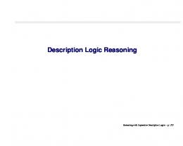
An usual assumption in databases is that one of a finite universe. This Section shows that temporal class diagrams do not enjoy the finite model property (FMP, for short). This means that reasoning on finite models is different from reasoning on infinite ones as proved by the following theorem. Theorem 6.1. Temporal class diagrams do not have the FMP. Proof. Let us consider the schema, Σinf , of Figure 6. We show that C0 is satisfiable only B(t ) on models with infinite objects. Let B be a model of Σinf such that ∃e0 ∈ ∆B .e0 ∈ C0 0 , B(t ) for some t0 ∈ T . Thus, ∃e1 ∈ ∆B .(he0 , e1 i ∈ RB(t0 ) ∧ e1 ∈ C1 0 ). Then, given the B(t ) dynamic extension, ∃t1 > t0 .e1 ∈ C2 1 , while, given the persistency and the disjointness B(t) B(t) constraints, ∀t > t1 .e1 6∈ C2 , and then, ∀t ≥ t1 .e1 6∈ C1 . Now, since C0 is snapshot, B(t) B(t ) e0 ∈ C0 for all t ∈ T , and, in particular, e0 ∈ C0 1 , while since C0 totally participates B(t ) B(t ) B(t ) in R, then, ∃e01 ∈ ∆B .(he0 , e01 i ∈ RB(t1 ) ∧ e01 ∈ C1 1 ). Since e01 ∈ C1 1 , while e1 6∈ C1 1 , B(t) then, e01 6= e1 . For similar reasons, ∃t2 > t1 such that ∀t ≥ t2 .e01 6∈ C1 . Thus, we need to introduce a new object, e001 to make C0 satisfiable, and so on so forth. 2 We are now able to show the second relevant result of this paper. The following theorem shows that the undecidability result also holds when reasoning w.r.t. finite models in temporal class diagrams.

16

A. Artale / Undecidability of Temporal Class Diagrams

Top s

d

C0 s

(1,n)

R

C1

dex

C2

per

C3

Figure 6. The Σinf schema.

Theorem 6.2. Reasoning over temporal class diagrams using persistency and dynamic constructs is undecidable even when considering legal temporal databases with finite domains. Proof. Obviously, also ALC F lacks the FMP. We then show that concept satisfiability w.r.t. an ALC F knowledge base is undecidable even considering finite models. The new ALC F axioms could be captured by temporal class diagrams by adopting the mapping already used in Theorem 5.2. Given a Turing machine, M = hA, S, ρi, we construct an ALC F KB, say KBf in , with a concept that is satisfiable w.r.t. KBf in iff the machine M does halt. The same notation introduced in Theorem 5.1 is used here. KBf in contains the following axioms: C0 v C£ u 3+ Chs0 ,bi u Chalt 0

(19)

discover(C, {Cx | x ∈ A }) Chalt v 3+ S1 t ∃R.Chalt next(C£ , D1 ) next(D1 , D2 ) Chs0 ,bi v D1

(20) (21) (22) (23) (24)

Chs0 ,bi v 2+ Cb discover(Cs , {Chs,ai | hs, ai ∈ S × A}) next(Cl , Cs ) next(Cs , Cr ) next(Cr , D3 ) C£ v Cl t 3+ Cl Cl v Cα → ∀R.Cα0 Cs v Cβ → ∀R.Cβ 0 Cr v Cγ → ∀R.Cγ 0 Ca v (¬Cl u ¬Cs u ¬Cr ) → ∀R.Ca , ∀a ∈ A ∪ {£} discover(S1, {Chs1 ,ai | a ∈ A ∪ {£}})

(25) (26) (27) (28) (29) (30) (31) (32) (33) (34) (35)

Chalt v 3+ Chain next(Chain , D4 ) D4 v ∀R.Chain

(36) (37) (38)

with axioms (31–33) for each instruction δ(α, β, γ) = hα0 , β 0 , γ 0 i. We now prove that C0 is satisfiable w.r.t. KBf in iff M has a finite computation starting from the empty tape. I(t ) “⇒” Let C0 be satisfiable, then, ∃hx0 , t0 i ∈ ∆I ×T .x0 ∈ C0 0 . Then, by axiom (19), I(t ) I(t ) I(t +1) x0 ∈ Chalt0 , and, by axioms (36,37), ∃t1 > t0 .(x0 ∈ Chain1 ∧x0 ∈ D4 1 ). By axiom (21),

A. Artale / Undecidability of Temporal Class Diagrams

17

I(t )

0

either x0 ∈ S1I(t0 ) for some t00 > t0 , or ∃x1 ∈ ∆I .(hx0 , x1 i ∈ RI(t0 ) ∧x1 ∈ Chalt0 ). If the last is true, we then show that x0 6= x1 . Indeed, since R is global, then, hx0 , x1 i ∈ RI(t1 +1) , and, I(t) I(t ) I(t +1) by axiom (38), x1 ∈ Chain1 , and by axiom (37), ∀t 6= t1 +1.x1 6∈ Chain . Since x0 ∈ Chain1 , then, x0 6= x1 . Thus, there is a chain of different objects in ∆I , hx0 , x1 , . . . , xn i, with n ≥ 0, 0 I(t ) such that x0 ∈ C0 0 , and, xn ∈ S1I(tn ) , for some t0n > t0 . The chain is finite since ∆I is finite. The fact that the chain hx0 , x1 , . . . , xn i represents a computation of M can be done similarly to Theorem 5.1. “⇐” Conversely, suppose that M is a Turing machine and hc0 , . . . , cn i its finite com. putation starting with the empty tape. We construct a model I = hT , ∆I , ·I(t) i of KBf in such that C0 is satisfiable. In particular, we fix T = hN, 0, Chalt = ∆I , and Chalt = ∅, for all j > 0. Furthermore, ∀j ∈ N: I(j)

= {i ∈ ∆I | the jth cell of ci contains x},

I(j)

= {i ∈ ∆I | the jth cell of ci is the active one}

I(j)

= Cs

I(j)

= Cs

• Cx • Cs • Cl

• Cr

I(j+1) I(j−1)

• C I(j) = I(j)

• Chain

I(j)

S

Cx  {j − 1} if j ∈ {1, . . . , n} = ∅ otherwise x∈A0

I(j)

= C£

I(j)

= D1

I(j)

= Cr

I(j)

= Chain

• D1

• D2

• D3

• D4

for all x ∈ A0

I(j−1) I(j−1)

I(j−1)

• S1I(j) =

I(j−1)

S

a∈A

I(j)

Chs1 ,ai .

It is easy to verify that I is a model of KBf in where C0 is satisfiable. 7.

2

Conclusions

We formally introduced a data modeling language useful to represent time-varying data. The language is equipped with a linear and graphical syntax and a model-theoretic semantics. A relevant aspect of the proposed formalism is the possibility to formally specify reasoning tasks based on the associated semantics. Reasoning problems as class, relationship and schema satisfiability and logical implication have been described. We then investigated the complexity of reasoning on temporal models and we found that such problem is undecidable as soon as the language is able to distinguish between temporal and atemporal constructs (in particular, whether the language captures temporal relationships) and has the ability to represent dynamic constraints between classes. While temporal class diagrams do not enjoy the finite model property we prove that even reasoning on finite models is undecidable. The main reason behind the undecidability result is the possibility to postulate that a binary relation does not vary in time. Indeed, it has been shown in [5] that temporal diagrams expressed in the ERV T modeling language can be embedded into the temporal description logic DLRU S . While DLRU S is undecidable, the fragment, DLR− U S , of DLRU S deprived of the ability to talk about temporal persistence of n-ary relations, for n ≥ 2, is decidable. Indeed, reasoning in DLR− U S is an EXPTIME-complete problem [5].

18

A. Artale / Undecidability of Temporal Class Diagrams

This result gives us an useful scenario where reasoning over temporal schemas becomes decidable. In particular, if we forbid timestamping for relationships (i.e., relationships are just unmarked) reasoning on temporal models with both concept timestamping and full evolution constraints can be reduced to reasoning over DLR− U S . The problem of reasoning in this setting is complete for EXPTIME since the EXPTIME-complete problem of reasoning with ALC knowledge bases can be captured by such schemas [7]. It is an open problem whether reasoning is still decidable by regaining timestamping for relationships (and maintaining timestamping for classes) but dropping evolution constraints altogether. We have a strong feeling that this represents a decidable scenario since it is possible to encode temporal schemas without evolution constraints by using a combination between the description logic DLR and the epistemic modal logic S5. Decidability results have been proved for the sub-logic ALC S5 [12]. But, it is an open problem whether this result still holds for the more complex logic DLRS5 . Acknowledgments The author would like to thank Diego Calvanese, Enrico Franconi, Sergio Tessaris and Frank Wolter for enlightening comments on earlier drafts of the paper. The author has been partially supported by the EU projects KnowledgeWeb, Interop and Tones.

References [1] A. Artale and E. Franconi. Temporal ER modeling with description logics. In Proc. of the International Conference on Conceptual Modeling (ER’99). Lecture Notes in Computer Science, Springer-Verlag, 1999. [2] A. Artale and E. Franconi. A survey of temporal extensions of description logics. Annals of Mathematics and Artificial Intelligence, 30(1-4), 2001. [3] Alessandro Artale. Reasoning on temporal conceptual schemas with dynamic constraints. In 11th International Symposium on Temporal Representation and Reasoning (TIME04). IEEE Computer Society, 2004. Also in Proc. of the 2004 International Workshop on Description Logics (DL’04). [4] Alessandro Artale, Enrico Franconi, and Federica Mandreoli. Description logics for modelling dynamic information. In Jan Chomicki, Ron van der Meyden, and Gunter Saake, editors, Logics for Emerging Applications of Databases. Lecture Notes in Computer Science, Springer-Verlag, 2003. [5] Alessandro Artale, Enrico Franconi, Frank Wolter, and Michael Zakharyaschev. A temporal description logic for reasoning about conceptual schemas and queries. In S. Flesca, S. Greco, N. Leone, and G. Ianni, editors, Proceedings of the 8th Joint European Conference on Logics in Artificial Intelligence (JELIA-02), volume 2424 of LNAI, pages 98–110. Springer, 2002. [6] F. Baader, D. Calvanese, D. McGuinness, D. Nardi, and P. F. Patel-Schneider, editors. Description Logic Handbook: Theory, Implementation and Applications. Cambridge University Press, 2002. [7] Daniela Berardi, Diego Calvanese, and Giuseppe De Giacomo. Reasoning on UML class diagrams. Artificial Intelligence, 168(1–2):70–118, 2005. [8] D. Calvanese, G. De Giacomo, and M. Lenzerini. On the decidability of query containment under constraints. In Proc. of the 17th ACM SIGACT SIGMOD SIGART Sym. on Principles of Database Systems (PODS’98), pages 149–158, 1998. [9] D. Calvanese, M. Lenzerini, and D. Nardi. Unifying class-based representation formalisms. J. of Artificial Intelligence Research, 11:199–240, 1999. [10] J. Chomicki and D. Toman. Temporal logic in information systems. In J. Chomicki and G. Saake, editors, Logics for Databases and Information Systems, chapter 1. Kluwer, 1998. [11] R. Elmasri and S. B. Navathe. Fundamentals of Database Systems. Benjamin/Cummings, 2nd edition, 1994. [12] D. Gabbay, A.Kurucz, F. Wolter, and M. Zakharyaschev. Many-dimensional modal logics: theory and applications. Studies in Logic. Elsevier, 2003. [13] H. Gregersen and J.S. Jensen. Conceptual modeling of time-varying information. Technical Report TimeCenter TR-35, Aalborg University, Denmark, 1998. [14] H. Gregersen and J.S. Jensen. Temporal Entity-Relationship models - a survey. IEEE Transactions on Knowledge and Data Engineering, 11(3):464–497, 1999. [15] R. Gupta and G. Hall. Modeling transition. In Proc. of ICDE’91, pages 540–549, 1991.

A. Artale / Undecidability of Temporal Class Diagrams

19

[16] C. S. Jensen, J. Clifford, S. K. Gadia, P. Hayes, and S. Jajodia et al. The Consensus Glossary of Temporal Database Concepts. In O. Etzion, S. Jajodia, and S. Sripada, editors, Temporal Databases - Research and Practice, pages 367–405. Springer-Verlag, 1998. [17] C. S. Jensen and R. T. Snodgrass. Temporal data management. IEEE Transactions on Knowledge and Data Engineering, 111(1):36–44, 1999. [18] C. S. Jensen, M. Soo, and R. T. Snodgrass. Unifying temporal data models via a conceptual model. Information Systems, 9(7):513–547, 1994. [19] S. Spaccapietra, C. Parent, and E. Zimanyi. Modeling time from a conceptual perspective. In Int. Conf. on Information and Knowledge Management (CIKM98), 1998. [20] C. Theodoulidis, P. Loucopoulos, and B. Wangler. A conceptual modelling formalism for temporal database applications. Information Systems, 16(3):401–416, 1991. [21] F. Wolter and M. Zakharyaschev. Satisfiability problem in description logics with modal operators. In Proc. of the 6 th International Conference on Principles of Knowledge Representation and Reasoning (KR’98), pages 512–523, Trento, Italy, June 1998.